Multiple-Attribute Decision-Making Method Using Similarity Measures of Hesitant Linguistic Neutrosophic Numbers Regarding Least Common Multiple Cardinality


Department of Electrical Engineering and Automation, Shaoxing University, 508 Huancheng West Road, Shaoxing 312000, Zhejiang, China
*
Author to whom correspondence should be addressed.
Symmetry 2018, 10(8), 330; https://doi.org/10.3390/sym10080330
Submission received: 10 July 2018
/
Revised: 5 August 2018
/
Accepted: 7 August 2018
/
Published: 9 August 2018
(This article belongs to the Special Issue Fuzzy Techniques for Decision Making 2018)
Abstract
:Linguistic neutrosophic numbers (LNNs) are a powerful tool for describing fuzzy information with three independent linguistic variables (LVs), which express the degrees of truth, uncertainty, and falsity, respectively. However, existing LNNs cannot depict the hesitancy of the decision-maker (DM). To solve this issue, this paper first defines a hesitant linguistic neutrosophic number (HLNN), which consists of a few LNNs regarding an evaluated object due to DMs’ hesitancy to represent their hesitant and uncertain information in the decision-making process. Then, based on the least common multiple cardinality (LCMC), we present generalized distance and similarity measures of HLNNs, and then develop a similarity measure-based multiple-attribute decision-making (MADM) method to handle the MADM problem in the HLNN setting. Finally, the feasibility of the proposed approach is verified by an investment decision case.
1. Introduction
In the real world, the linguistic expression is well-suited for the thinking and expressing patterns of human beings. Due to the vagueness of languages and the complexity of decision-making environments, the linguistic fuzzy theory has been well developed in the past decades and shows irreplaceable advantages in the fuzzy decision-making field. Linguistic variables (LVs) were defined for fuzzy reasoning and decision-making [1,2,3,4]. Linguistic uncertain variables [5,6] (interval-valued linguistic variables) were then defined to depict uncertain linguistic information in decision-making problems [7,8]. After that, a linguistic intuitionistic fuzzy number (LIFN) [9], which contains two independent LVs to describe the degrees of truth and falsity, respectively, was presented to handle the uncertainty and incompleteness in linguistic decision-making environments [10]. Furthermore, with the wide application of the neutrosophic theory in decision-making [11,12,13], Fang and Ye [14] proposed a linguistic neutrosophic number (LNN) by adding a new LV to the LIFN for representing the indeterminacy degree to do with the indeterminate and inconsistent linguistic information [15]. Although there exist some research works on LNNs [14,15], existing LNNs cannot depict the hesitancy of decision-makers (DMs) in the linguistic assessment of alternatives.
Concerning the handling of the human hesitant cognition in decision-making environments, many works have been published so far. Torra and Narukawa [16] and Torra [17] originally introduced hesitant fuzzy sets (HFSs) to express the hesitancy by allowing the membership to contain several possible values. Then, for linguistic decision-making problems, the expression of a hesitant fuzzy linguistic set (HFLS) [18] was obtained based on combining a linguistic term (LT) set with a HFS so as to satisfy the hesitant linguistic evaluation requirements [19,20] of DMs. After that, an interval-valued HFLS [21] was presented as an extension form by combining an interval-valued LT set with a HFS. Recently, Ye [22] proposed the hesitant neutrosophic linguistic number (HNLN) to carry out hesitant decision-making problems with the neutrosophic linguistic number that contains partial determinacy and partial indeterminacy. However, there is no definition or decision-making method for the hesitant sets of LNNs in the existing literature. Additionally, in the hesitant linguistic expressions of DMs, the components between two hesitant sets generally have difference in their length sizes, and thus it is difficult to directly perform measure calculations between hesitant sets. Thus, several researchers have proposed some extension methods to extend the shorter items in the two hesitant sets by adding the minimum values, maximum values, or any values [23,24] to reach their identical length. However, these extension methods depend too much on the subjective preferences and interests of the DMs. To solve this problem, we have already introduced the least common multiple cardinality (LCMC) to extend the hesitant fuzzy elements in our previous research works [22,25], which become more objective for the decision-making calculation of HFSs.
As aforementioned, there is a gap of hesitant LNNs in existing studies. For instance, suppose that we hesitate between two single-valued LNNs, <h7, h3, h4> and <h5, h3, h1>, from the given LT set H = {hs|s [0, 8]} regarding an evaluated object. However, it is difficult to express the hesitation information and the LNN information of the DMs simultaneously by a unique LNN or a unique HFS. Therefore, for the purposes of satisfying the demand of hesitant decision-making with LNNs and ensuring the objectivity of the measure calculation, this paper aims to (i) define the concept of HLNNs by combining HFSs with LNNs, (ii) present the LCMC-based generalized distance and similarity measures of HLNNs for more objective measure calculation of HLNN information, and (iii) to propose a novel multiple-attribute decision-making (MADM) method based on the proposed LCMC-based similarity measure in the HLNN setting.
In order to do so, Section 2 briefly reviews LNNs. Section 3 defines a HLNN and a HLNN set. Then, in Section 4, the LCMC-based generalized distance and similarity measures of HLNNs are presented. In Section 5, a new MADM method was developed by using the proposed similarity measure of HLNNs. In Section 6, the feasibility of the proposed approach is demonstrated by an investment case. The conclusions and future research of HLNNs are discussed in the last section.
2. Linguistic Neutrosophic Numbers (LNNs)
Fang and Ye [14] originally presented the following definition of the LNN:
Definition 1
([14]). Let H = {h0, h1, ..., hτ} be a LT set, where τ + 1 is an odd cardinality. A LNN can be defined as ϑ = < hT, hU, hF> for hT, hU, hF H and T, U, F [0, τ], where hT, hU, hF represent the degrees of truth, indeterminacy, and falsity, respectively.
For the comparison of LNNs, the score and accuracy functions of LNNs are defined as follows [14]:
Definition 2
([14]). Let ϑ = <hT, hU, hF> be a LNN in H. Then its score function can be given by:
and its accuracy function can be expressed as
Definition 3
- (1)
- If S(ϑα) < S(ϑβ), then ϑα < ϑβ;
- (2)
- If S(ϑα) > S(ϑβ), then ϑα > ϑβ;
- (3)
- If S(ϑα) = S(ϑβ) and V(ϑα) < V(ϑβ), then ϑα < ϑβ;
- (4)
- If S(ϑα) = S(ϑβ) and V(ϑα) > V(ϑβ), then ϑα > ϑβ;
- (5)
- If S(ϑα) = S(ϑβ) and V(ϑα) = V(ϑβ), then ϑα = ϑβ.
3. Hesitant Linguistic Neutrosophic Numbers (HLNNs) and HLNN Set
Definition 4
By integrating HFS with LNN, we define a HLNN set as follows:
Definition 5.
Set a universe of discourse S = {s1, s2, …, sq} and a finite LT set H = {h0, h1, …, hτ}, and then a HLNN set Nl on S can be expressed as
where El(sj) is a set of mj LNNs, denoted by a HLNNfor sjS.
4. LCMC-Based Distance and Similarity Measures of HLNNs
In most situations, the cardinal numbers (the number of LNNs) of HLNNs evaluated for the same object are usually different. Thus, it is necessary to make the cardinal numbers of the two HLNNs the same to satisfy the distance and similarity measures between them.
We assume that p HLNNs on S = {s1, s2, …, sq} are for sj S (j = 1, 2, ..., q). Then, the HLNNs for i = 1, 2, …, p can be given by
where mij is the cardinal number of (i = 1, 2, …, p and j = 1, 2, …, q).
Provided that the LCMC of mij (i = 1, 2, ..., p and j = 1, 2, ..., q) is cj (j = 1, 2, …, q), by increasing the number of LNNs (k = 1, 2, ..., mij) in depending on cj (j = 1, 2, …, q), the extended HLNN (i = 1, 2, …, p and j = 1, 2, …, q) will be obtained by the extension forms:
where Rij is the number of LNNs (k = 1, 2, ..., mij) in (i = 1, 2, …, p and j = 1, 2, …, q), calculated by:
Additionally, the elements (k = 1, 2, …, cj) in are arranged in an ascending order, denoted as (i = 1, 2, …, p and j = 1, 2, …, q), where is a permutation satisfying (k = 1, 2, …, cj).
Definition 6.
Letandbe two HLNN sets on S = {s1, s2, ..., sq}, whereand(j = 1, 2, …, q) are HLNNsin a LT set H = {h0, h1, ..., hτ} for hjH. Let f(hj) = j/τ be a linguistic scale function. Then, the normalized generalized distance betweenandcan be represented as:
Obviously, degenerates to the normalized generalized distance of Hamming for ρ = 1 and to the normalized generalized distance of Euclidean for ρ = 2.
For the generalized distance , there is a proposition as follows:
Proposition 1.
For any two HLNN setsand, the generalized distancebetweenandfor ρ > 0 contains the following properties:
- (HP1)
- ;
- (HP2)
- if and only if;
- (HP3)
- ;
- (HP4)
- Letbe a HLNN set, thenandif.
Proof.
It is obvious that the properties (HP1)–(HP3) are satisfied for . Thus, we only need to prove the property (HP4).
Since there is , there exists for sj S (j = 1, 2, ..., q), which implies , , for k = 1, 2, ..., cj. It follows that
Then there are the following inequalities:
Thus, the following relations can be further obtained:
By Equation (4), there are and for ρ > 0. Therefore, the property (HP4) can hold. □
If we consider the weight wj of an element sj S with wj [0, 1] and , the generalized weighted distance between and is
Since the measures of similarity and distance are complementary with each other, the weighted measure of similarity between and can be represented by
Similar to the properties (HP1)–(HP4) satisfied by the generalized distance measure in Proposition 1, the similarity measure also has the proposition as follows:
Proposition 2.
The similarity measurefor ρ > 0 contains the following properties:
- (HP1)
- ;
- (HP2)
- if and only if;
- (HP3)
- ;
- (HP4)
- Letbe a HLNN set, then there areandif.
Proof.
It is clear that satisfies the properties (SP1)–(SP3). Thus, we only prove the property (SP4) here.
According to the proved property (HP4) in Proposition 1, if , there exists the relations of and for ρ > 0. Since the similarity measure is the complement of the distance measure, both and can be easily obtained. Therefore, the property (SP4) can hold. □
5. MADM Method Using the Similarity Measure of HLNNs
For a MADM problem in the HLNN setting, some DMs need to evaluate p alternatives (denoted by G = {g1, g2, …, gp}) over q attributes (denoted by S = {s1, s2, …, sq}) from the LT set H = {h0, h1, …, hτ}. Then, a weight vector W = (ω1, ω2, …, ωq), which is on the conditions of 0 ≤ ωj ≤ 1 (j = 1, 2, ..., q) and , represents the importance of the attributes in S. Thus, the HLNN decision matrix M can be expressed as:
where is a HLNN for sj S, and mij is the number of LNNs in (i = 1, 2, …, p and j = 1, 2, …, q).
On the basis of the proposed similarity measure, a novel MADM method of HLNN is presented by the following steps:
Step 1: For any HLNN (j = 1, 2, …, q) in M, rank all elements (k = 1, 2, …, mij) in each HLNN (j = 1, 2, …, q) in an ascending order according to their score and accuracy functions, then yield the corresponding extended HLNN based on the LCMC cj and the occurrence number Rij of every LNN in obtained by Equation (3). Hence, the extended decision matrix is
where (i = 1, 2, …, p and j = 1, 2, …, q) satisfies (k = 1, 2, …, cj).
Step 2: Specify an ideal HLNN set as for all (k = 1, 2, ..., cj and j = 1, 2, ..., q).
Hence, the similarity measure between gi (i = 1, 2, …, p) and g* can be calculated by
Step 3: According to the similarity measure results, rank the alternatives in G = {g1, g2, …, gm} in a descending order and choose the best one.
Step 4: End.
HLNN is a hybrid form of a LNN and HFS, which inherits the advantages of both the LNN and HFS, and expresses the decision-making information with a hesitant set of LNNs. The proposed LCMC-based distance and similarity measures can deal with not only the HLNN information, but also the LNN information, because the LNN is only a special case of the HLNN when the DMs have no hesitation; while all existing aggregation operators of LNNs [14] cannot aggregate HLNN information for the reason that the HLNN is a LNN set of any length. Furthermore, existing MADM methods cannot deal with decision-making problems in the HLNN setting.
Moreover, to ensure the objectivity of the measure calculational results, the proposed LCMC-based distance and similarity measures are based on the LCMC extension method in HLNNs rather than by simply adding special components, such as the maximum or the minimum or the average values, which heavily depend on the personal interests and preferences of DMs [23,24] so as to easily result in subjective decision-making results. Thus, the novel MADM method of HLNN provides a more general and objective decision-making process for decision-makers.
6. Actual Example
In this section, to verify whether the novel MADM approach with HLNNs is feasible and reasonable in practical applications, an investment decision-making case adapted from [14] is illustrated under a HLNN environment. In this case, the investment company makes an optimal selection in a set of four possible manufacturers, G = {g1, g2, g3, g4}, for producing computers (g1), cars (g2), food (g3), and clothing (g4), respectively. The four alternatives must satisfy a set of three attributes, S = {s1, s2, s3}, including the risk (s1), the growth (s2), and the environmental impact (s3), with the importance given by the weight vector W = (0.35, 0.25, 0.4). Now, some DMs are assigned to assess the alternatives over the attributes by HLNN expressions from the given LT set H = {h0: none, h1: lowest, h2: lower, h3: low, h4: moderate, h5: high, h6: higher, h7: highest, h8: perfect}. Then, the assessment results regarding the four alternatives g1, g2, g3, and g4 on the three attributes s1, s2, and s3 can be constructed as
Thus, there are the following decision steps:
Step 1: According to the score and accuracy functions obtained by Equations (1) and (2), rank the LNNs (k = 1, 2, …, mij) in each HLNN (i = 1, 2, 3, 4 and j = 1, 2, 3) in an ascending order, and obtain the following matrix:
Then, according to the LCMC cj = 6 (j = 1, 2, 3) and the number of occurrences of LNNs Rij of (i = 1, 2, 3, 4 and j = 1, 2, 3) obtained by Equation (3), yield the following extended decision matrix :
Step 2: Obtain the similarity measures between the alternatives g1, g2, g3, and g4 and the ideal solution g* = {{<8,0,0>, <8,0,0>, <8,0,0>, <8,0,0>, <8,0,0>, <8,0,0>}, {<8,0,0>, <8,0,0>, <8,0,0>, <8,0,0>, <8,0,0>, <8,0,0>}, {<8,0,0>, <8,0,0>, <8,0,0>, <8,0,0>, <8,0,0>, <8,0,0>}} by Equation (7) for ρ = 1 and 2:
Step 3: Due to Sw(g4, g*) > Sw(g2, g*) > Sw(g3, g*) > Sw(g1, g*) for ρ = 1 and 2, the ranking of the four alternatives is g4 > g2 >g3 > g1; thus, the best choice is g4.
By following the above steps, the MADM calculations of ρ [3, 100] are further performed for this example. The relative decision results, including the similarity measure, ranking order, average value (AV), standard deviation (SD), and the best alternative, are shown in Table 1. Obviously, the ranking order is g4 > g2 > g3 > g1 for ρ = 1 and 2, and then it becomes g4 > g3 > g2 > g1 for ρ > 2; while the best alternative is always g4.
7. Discussion and Analysis
In this section, further discussion and analysis are carried out for the resolution and the sensitivity of the novel MADM method of HLNNs.
7.1. Resolution Analysis
According to Table 1, Figure 1 illustrates the SDs of the similarity measures for ρ [1, 100]. Clearly, the SD increases with increasing the value of ρ. Then, it reaches 0.051 for ρ = 100. Since the SD can reflect the resolution/discrimination level of the MADM method, it is obvious that the resolution/discrimination level will be enhanced with increasing the value of ρ so as to provide effective decision information for decision-makers in the MADM process. However, considering that the computational complexity of MADM increases with increasing the value of ρ, we recommend selecting the MADM method with some suitable value of ρ under the condition that the resolution degree meets some actual requirement and the DMs’ preference.
7.2. Sensitivity Analysis of Weights
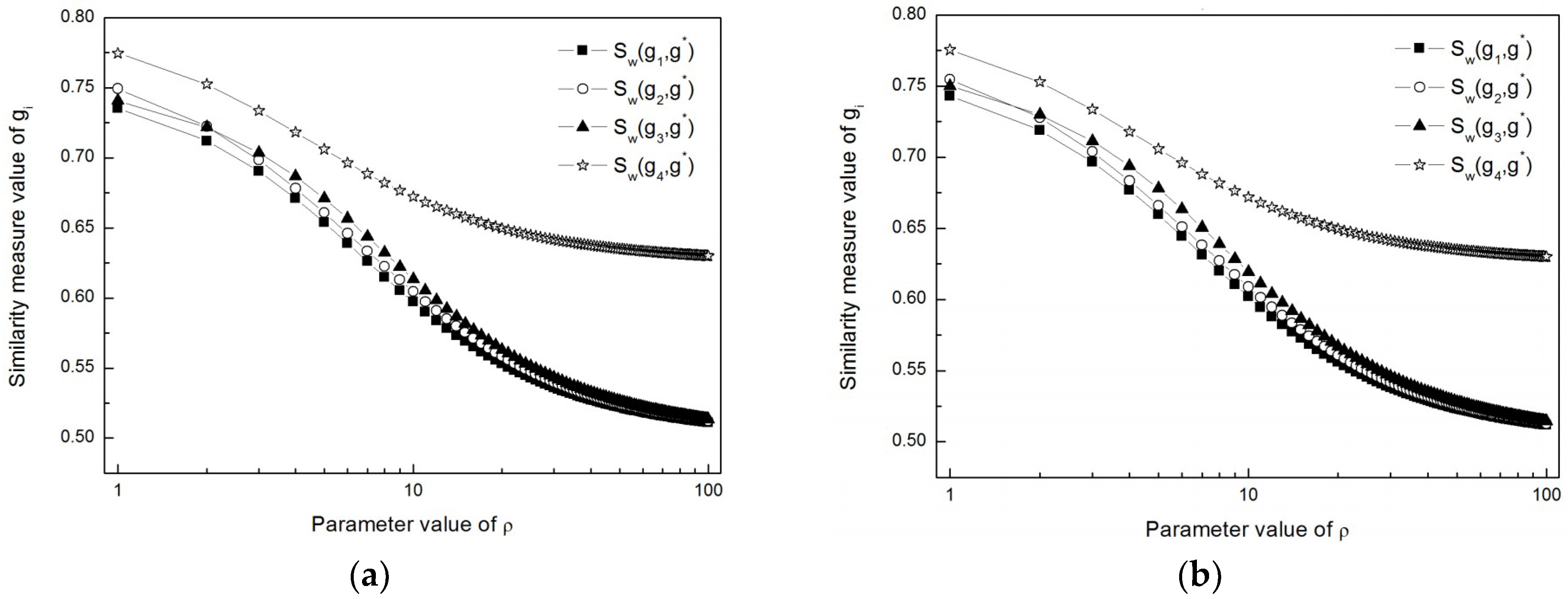
The average weight vector of W = (1/3, 1/3, 1/3) is applied to the actual example as a comparison with W = (0.35, 0.25, 0.4) to illustrate the weight sensitivity of the MADM method. The decision results with W = (1/3, 1/3, 1/3) are shown in Table 2. Then, the similarity measure values for W = (0.35, 0.25, 0.4) and W = (1/3, 1/3, 1/3) are further illustrated in Figure 2a,b.
From Figure 2, obviously, the similarity measure curves with W = (0.35, 0.25, 0.4) are very similar to those with W = (1/3, 1/3, 1/3). By carefully comparing Table 1 and Table 2, we find that the ranking orders are identical except that of ρ = 2. For ρ = 2, the ranking orders of g4 > g2 > g3 > g1 for W = (0.35, 0.25, 0.4) and g4 > g3 > g2 > g1 for W = (1/3, 1/3, 1/3) indicate a little difference. Then, the best alternatives are the same within the entire range of ρ. Hence, the ranking orders in this example imply a little sensitivity to the attribute weights.
8. Conclusions
This paper firstly defined the concept of HLNNs by integrating a HFS with a LNN. Then, the normalized generalized distance and similarity measures of HLNNs were presented based on the LCMC method. Next, a novel MADM method based on the proposed similarity measure was presented under the HLNN environment. Finally, a MADM example of an investment problem was illustrated to demonstrate that the developed method is feasible and applicable. Since the HLNN combines the merits of the HFS and LNN, containing more information than the LNN, the MADM method of HLNNs based on the LCMC method is more objective and more suitable for the practical applications with HLNN information.
However, some advantages of the proposed HLNNs and MADM method based on the LCMC method are listed as follows:
- (1)
- The proposed HLNN provides a new effective way to express more decision information than existing LNNs by considering the hesitancy of DMs.
- (2)
- The proposed MADM method of HLNNs solves the MADM problems with HLNN information for the first time, as well as the gap of existing linguistic decision-making methods.
- (3)
Future research on HLNNs will focus on the development of new aggregation operators and correlation coefficients of HLNNs, and their applications in fault diagnosis, medical diagnosis, decision-making, and so on in the HLNN setting.
Author Contributions
J.Y. originally proposed HLNNs and their operations, and W.C. presented the MADM method of HLNNs and the calculation and comparative analysis of an actual example. Both coauthors wrote the paper together.
Funding
This paper was supported by the National Natural Science Foundation of China (No. 61703280).
Conflicts of Interest
The authors declare no conflict of interest.
References
- Zadeh, L.A. The concept of a linguistic variable and its application to approximate reasoning Part I. Inf. Sci. 1975, 8, 199–249. [Google Scholar] [CrossRef]
- Herrera, F.; Herrera-Viedma, E.; Verdegay, J.L. A model of consensus in group decision making under linguistic assessments. Fuzzy Set Syst. 1996, 78, 73–87. [Google Scholar] [CrossRef]
- Herrera, F.; Herrera-Viedma, E. Linguistic decision analysis: Steps for solving decision problems under linguistic information. Fuzzy Set Syst. 2000, 115, 67–82. [Google Scholar] [CrossRef]
- Xu, Z.S. A method based on linguistic aggregation operators for group decision making with linguistic preference relations. Inf. Sci. 2004, 166, 19–30. [Google Scholar] [CrossRef]
- Xu, Z.S. Uncertain linguistic aggregation operators based approach to multiple attribute group decision making under uncertain linguistic environment. Inf. Sci. 2004, 168, 171–184. [Google Scholar] [CrossRef]
- Xu, Z.S. Induced uncertain linguistic OWA operators applied to group decision making. Inf. Sci. 2006, 7, 231–238. [Google Scholar] [CrossRef]
- Wei, G.W. Uncertain linguistic hybrid geometric mean operator and its application to group decision making under uncertain linguistic environment. Int. J. Uncertain. Fuzziness 2009, 17, 251–267. [Google Scholar] [CrossRef]
- Peng, B.; Ye, C.; Zeng, S. Uncertain pure linguistic hybrid harmonic averaging operator and generalized interval aggregation operator based approach to group decision making. Knowl.-Based Syst. 2012, 36, 175–181. [Google Scholar] [CrossRef]
- Chen, Z.C.; Liu, P.H.; Pei, Z. An approach to multiple attribute group decision making based on linguistic intuitionistic fuzzy numbers. Int. J. Comput. Intell. Syst. 2015, 8, 747–760. [Google Scholar] [CrossRef] [Green Version]
- Liu, P.D.; Liu, J.L.; Merigó, J.M. Partitioned Heronian means based on linguistic intuitionistic fuzzy numbers for dealing with multi-attribute group decision making. Appl. Soft Comput. 2018, 62, 395–422. [Google Scholar] [CrossRef]
- Peng, X.; Liu, C. Algorithms for neutrosophic soft decision making based on EDAS, new similarity measure and level soft set. J. Intell. Fuzzy Syst. 2017, 32, 955–968. [Google Scholar] [CrossRef]
- Zavadskas, E.K.; Bausys, R.; Juodagalviene, B.; Garnyte-Sapranaviciene, I. Model for residential house element and material selection by neutrosophic MULTIMOORA method. Eng. Appl. Artif. Intell. 2017, 64, 315–324. [Google Scholar] [CrossRef]
- Bausys, R.; Juodagalviene, B. Garage location selection for residential house by WASPAS-SVNS method. J. Civ. Eng. Manag. 2017, 23, 421–429. [Google Scholar] [CrossRef]
- Fang, Z.B.; Ye, J. Multiple attribute group decision-making method based on linguistic neutrosophic numbers. Symmetry 2017, 9, 111. [Google Scholar] [CrossRef]
- Liu, P.D.; Mahmood, T.; Khan, Q. Group decision making based on power Heronian aggregation operators under linguistic neutrosophic environment. Int. J. Fuzzy Syst. 2018, 20, 970–985. [Google Scholar] [CrossRef]
- Torra, V.; Narukawa, Y. On hesitant fuzzy sets and decision. In Proceedings of the 18th IEEE International Conference on Fuzzy Systems, Jeju Island, Korea, 20–24 August 2009; pp. 1378–1382. [Google Scholar] [CrossRef]
- Torra, V. Hesitant fuzzy sets. Int. J. Intell. Syst. 2010, 25, 529–539. [Google Scholar] [CrossRef]
- Rodríguez, R.M.; Martínez, L.; Herrera, F. Hesitant Fuzzy Linguistic Term Sets for Decision Making. IEEE Trans. Fuzzy Syst. 2012, 20, 109–119. [Google Scholar] [CrossRef] [Green Version]
- Rodríguez, R.M.; MartíNez, L.; Herrera, F. A group decision making model dealing with comparative linguistic expressions based on hesitant fuzzy linguistic term sets. Inf. Sci. 2013, 241, 28–42. [Google Scholar] [CrossRef]
- Lin, R.; Zhao, X.F.; Wei, G.W. Models for selecting an ERP system with hesitant fuzzy linguistic information. J. Intell. Fuzzy Syst. 2014, 26, 2155–2165. [Google Scholar] [CrossRef]
- Wang, J.Q.; Wu, J.T.; Wang, J.; Zhang, H.; Chen, X. Interval-valued hesitant fuzzy linguistic sets and their applications in multi-criteria decision-making problems. Inf. Sci. 2014, 288, 55–72. [Google Scholar] [CrossRef]
- Ye, J. Multiple Attribute Decision-Making Methods Based on the Expected Value and the Similarity Measure of Hesitant Neutrosophic Linguistic Numbers. Cogn. Comput. 2018, 10, 454–463. [Google Scholar] [CrossRef]
- Zhu, B.; Xu, Z. Consistency Measures for Hesitant Fuzzy Linguistic Preference Relations. IEEE Trans. Fuzzy Syst. 2014, 22, 35–45. [Google Scholar] [CrossRef]
- Liao, H.; Xu, Z.; Zeng, X.J.; Merigó, J.M. Qualitative decision making with correlation coefficients of hesitant fuzzy linguistic term sets. Knowl.-Based Syst. 2015, 76, 127–138. [Google Scholar] [CrossRef]
- Ye, J. Multiple-attribute Decision-Making Method under a Single-Valued Neutrosophic Hesitant Fuzzy Environment. J. Intell. Syst. 2014, 24, 23–36. [Google Scholar] [CrossRef]
Figure 1.
SD of similarity measure values for ρ [1, 100] and W = (0.35, 0.25, 0.4).
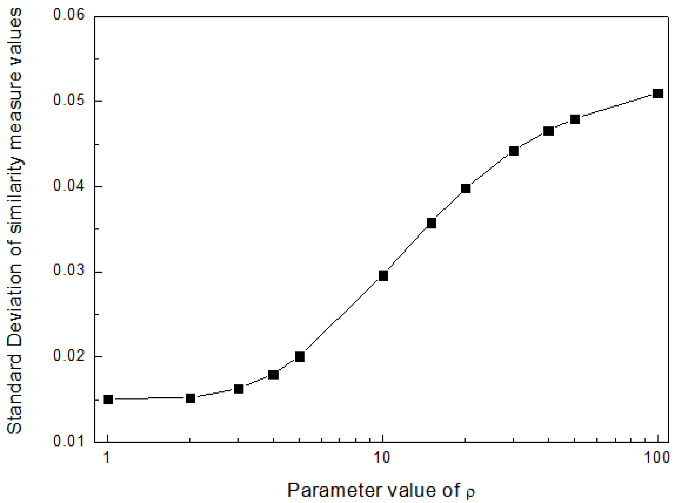
Figure 2.
Similarity measure values of four alternatives for ρ [1, 100]. (a) W = (0.35, 0.25, 0.4) and (b) W = (1/3, 1/3, 1/3).
Figure 2.
Similarity measure values of four alternatives for ρ [1, 100]. (a) W = (0.35, 0.25, 0.4) and (b) W = (1/3, 1/3, 1/3).

Table 1.
Decision results of the proposed multiple-attribute decision-making (MADM) method for ρ [1, 100] and W = (0.35, 0.25, 0.4).
Table 1.
Decision results of the proposed multiple-attribute decision-making (MADM) method for ρ [1, 100] and W = (0.35, 0.25, 0.4).
| ρ1 | Sw(g1, g*), Sw(g2, g*), Sw(g3, g*), Sw(g4, g*) 2 | Ranking Order | AV 3 | SD 4 | Best Alternative |
|---|---|---|---|---|---|
| 1 | 0.7354, 0.7493, 0.7406, 0.7747 | g4 > g2 > g3 > g1 | 0.7500 | 0.0151 | g4 |
| 2 | 0.7121, 0.7224, 0.7217, 0.7525 | g4 > g2 > g3 > g1 | 0.7272 | 0.0152 | g4 |
| 3 | 0.6905, 0.6985, 0.7037, 0.7335 | g4 > g3 > g2 > g1 | 0.7066 | 0.0163 | g4 |
| 4 | 0.6710, 0.6781, 0.6867, 0.7182 | g4 > g3 > g2 > g1 | 0.6885 | 0.018 | g4 |
| 5 | 0.6539, 0.6608, 0.6710, 0.7061 | g4 > g3 > g2 > g1 | 0.6730 | 0.0201 | g4 |
| 10 | 0.5972, 0.6047, 0.6133, 0.6722 | g4 > g3 > g2 > g1 | 0.6219 | 0.0296 | g4 |
| 15 | 0.5690, 0.5754, 0.5817, 0.6575 | g4 > g3 > g2 > g1 | 0.5959 | 0.0358 | g4 |
| 20 | 0.5531, 0.5582, 0.5631, 0.6497 | g4 > g3 > g2 > g1 | 0.5810 | 0.0398 | g4 |
| 30 | 0.5361, 0.5397, 0.5432, 0.6417 | g4 > g3 > g2 > g1 | 0.5652 | 0.0443 | g4 |
| 40 | 0.5273, 0.5301, 0.5327, 0.6376 | g4 > g3 > g2 > g1 | 0.5569 | 0.0466 | g4 |
| 50 | 0.5220, 0.5242, 0.5264, 0.6351 | g4 > g3 > g2 > g1 | 0.5519 | 0.048 | g4 |
| 100 | 0.5111, 0.5123, 0.5134, 0.6301 | g4 > g3 > g2 > g1 | 0.5417 | 0.051 | g4 |
Notes: 1 ρ: parameter; 2 Sw(gi, g*): the similarity measures between the alternatives gi(i = 1, 2, 3, 4) and the ideal solution g* = {{<8,0,0>, <8,0,0>, <8,0,0>, <8,0,0>, <8,0,0>, <8,0,0>}, {<8,0,0>, <8,0,0>, <8,0,0>, <8,0,0>, <8,0,0>, <8,0,0>}, {<8,0,0>, <8,0,0>, <8,0,0>, <8,0,0>, <8,0,0>, <8,0,0>}}; 3 AV: average value; 4 SD: standard deviation.
Table 2.
Decision results of the proposed MADM method for ρ [1, 100] and W = (1/3, 1/3, 1/3).
| ρ | Sw(g1, g*), Sw(g2, g*), Sw(g3, g*), Sw(g4, g*) | Ranking Order | AV | SD | Best Alternative |
|---|---|---|---|---|---|
| 1 | 0.7431, 0.7546, 0.7500, 0.7755 | g4 > g2 > g3 > g1 | 0.7558 | 0.0121 | g4 |
| 2 | 0.7189, 0.7278, 0.7300, 0.7529 | g4 > g3 > g2 > g1 | 0.7324 | 0.0125 | g4 |
| 3 | 0.6968, 0.7039, 0.7112, 0.7336 | g4 > g3 > g2 > g1 | 0.7114 | 0.0138 | g4 |
| 4 | 0.6769, 0.6833, 0.6938, 0.7180 | g4 > g3 > g2 > g1 | 0.693 | 0.0156 | g4 |
| 5 | 0.6596, 0.6659, 0.6779, 0.7057 | g4 > g3 > g2 > g1 | 0.6773 | 0.0177 | g4 |
| 10 | 0.6019, 0.6088, 0.6193, 0.6717 | g4 > g3 > g2 > g1 | 0.6254 | 0.0274 | g4 |
| 15 | 0.5727, 0.5786, 0.5865, 0.6572 | g4 > g3 > g2 > g1 | 0.5988 | 0.0341 | g4 |
| 20 | 0.556, 0.5608, 0.5671, 0.6495 | g4 > g3 > g2 > g1 | 0.5834 | 0.0384 | g4 |
| 30 | 0.5381, 0.5415, 0.5459, 0.6415 | g4 > g3 > g2 > g1 | 0.5668 | 0.0432 | g4 |
| 40 | 0.5289, 0.5315, 0.5349, 0.6374 | g4 > g3 > g2 > g1 | 0.5582 | 0.0458 | g4 |
| 50 | 0.5232, 0.5254, 0.5281, 0.6350 | g4 > g3 > g2 > g1 | 0.5529 | 0.0474 | g4 |
| 100 | 0.5118, 0.5128, 0.5142, 0.6300 | g4 > g3 > g2 > g1 | 0.5422 | 0.0507 | g4 |
© 2018 by the authors. Licensee MDPI, Basel, Switzerland. This article is an open access article distributed under the terms and conditions of the Creative Commons Attribution (CC BY) license (http://creativecommons.org/licenses/by/4.0/).
Share and Cite
MDPI and ACS Style
Cui, W.; Ye, J. Multiple-Attribute Decision-Making Method Using Similarity Measures of Hesitant Linguistic Neutrosophic Numbers Regarding Least Common Multiple Cardinality. Symmetry 2018, 10, 330. https://doi.org/10.3390/sym10080330
AMA Style
Cui W, Ye J. Multiple-Attribute Decision-Making Method Using Similarity Measures of Hesitant Linguistic Neutrosophic Numbers Regarding Least Common Multiple Cardinality. Symmetry. 2018; 10(8):330. https://doi.org/10.3390/sym10080330
Chicago/Turabian StyleCui, Wenhua, and Jun Ye. 2018. "Multiple-Attribute Decision-Making Method Using Similarity Measures of Hesitant Linguistic Neutrosophic Numbers Regarding Least Common Multiple Cardinality" Symmetry 10, no. 8: 330. https://doi.org/10.3390/sym10080330
Note that from the first issue of 2016, this journal uses article numbers instead of page numbers. See further details here.