Perception of 3D Symmetrical and Nearly Symmetrical Shapes


1
Department of Electrical and Computer Engineering, Purdue University, West Lafayette, IN 47907, USA
2
School of Psychology, National Research University Higher School of Economics, Moscow 109316, Russia
3
Department of Cognitive Sciences, University of California-Irvine, Irvine, CA 92697, USA
*
Author to whom correspondence should be addressed.
Symmetry 2018, 10(8), 344; https://doi.org/10.3390/sym10080344
Submission received: 17 July 2018
/
Revised: 8 August 2018
/
Accepted: 13 August 2018
/
Published: 16 August 2018
(This article belongs to the Special Issue Symmetry-Related Activity in Mid-Level Vision)
Abstract
:The human visual system uses priors to convert an ill-posed inverse problem of 3D shape recovery into a well-posed one. In previous studies, we have demonstrated the use of priors like symmetry, compactness and minimal surface in the perception of 3D symmetric shapes. We also showed that binocular perception of symmetric shapes can be well modeled by the above-mentioned priors and binocular depth order information. In this study, which used a shape-matching task, we show that these priors can also be used to model perception of near-symmetrical shapes. Our near-symmetrical shapes are asymmetrical shapes obtained from affine distortions of symmetrical shapes. We found that the perception of symmetrical shapes is closer to veridical than the perception of asymmetrical shapes. We introduce a metric to measure asymmetry of abstract polyhedral shapes, and a similar metric to measure shape dissimilarity between two polyhedral shapes. We report some key observations obtained by analyzing the data from the experiment. A website was developed with all the shapes used in the experiment, along with the shapes recovered by the subject and the shapes recovered by the model. This website provides a qualitative analysis of the effectiveness of the model and also helps demonstrate the goodness of the shape metric.
1. Introduction
Research on human 3D shape perception started with two seminal papers published in the same year in the same journal [1,2]. The authors of these papers addressed the fundamental question in vision: how is the 3D percept of an object produced from a single 2D retinal image? Hans Wallach, who received his training with one of the founding fathers of Gestalt psychology, started his paper with a note of disappointment that, despite numerous attempts, no Gestalt psychologist, nor anyone else, was able to show how Prägnanz or the simplicity principle could produce veridical 3D percepts of shapes. So, he turned his attention to the competing tradition of empiricism, and set out to demonstrate that it is learning based on motion cues, rather than any innate simplicity predilection, that teaches human observers about the three-dimensionality of objects. Wallach and O’Connell showed that when the observer looks at a stationary shadow of an unstructured 3D polygonal line object, he never perceives a 3D shape. However, when the 3D object rotates, the changing shadow of the rotating object leads to a 3D percept (they called this “kinetic-depth-effect”). This way, Wallach and O’Connell provided evidence that motion, in the absence of any other cue, can produce a 3D percept. However, they did not explain how the 3D percept is actually produced by 2D motion cue. It was Hay [3], and later Ullman [4] and Longuet-Higgins [5], who formulated a mathematical and computational theory of kinetic depth effect. The computational theory is called, after Ullman [4], the structure from motion theorem (SFM). What was obvious to the authors of SFM and was not to Wallach and O’Connell, is that 3D shape cannot be computed from motion cue without a rigidity predilection or constraint. Indeed, all explanations of SFM rely on the assumption that the individual views are images of the same object and that the object is at least approximately rigid. So, in a sense, Wallach, who was looking for an empiristic theory of 3D vision, in which the role of simplicity constraints is minimal or absent altogether, ended up providing experimental evidence for the operation of such a constraint.
Simplicity constraint was an explicit motivation behind the second seminal contribution to our understanding of 3D shape perception that was mentioned in the previous paragraph [1]. Hochberg and McAlister used Kopfermann’s [6] observation on the role of viewing direction in perception of a 3D Necker (transparent) cube from a single 2D line drawing. They observed that a 3D cube, which is characterized by a high degree of simplicity or redundancy, is always perceived as a 3D shape, except for very special 2D views, which themselves are very simple. They, like Wallach and O’Connell, did not provide a computational theory of how the 3D percept is produced from a single 2D image, but their paper inspired others to continue research on the role of constraints in 3D shape perception [7,8,9,10,11,12]. We now know that constraints are absolutely essential in 3D shape recovery, because this recovery is an ill-posed inverse problem [13].
Forming a 2D retinal or camera image of a 3D shape is a forward problem, and it is described in the rules of geometrical optics. These rules are essentially equivalent to the rules of perspective projection, except for the facts that (i) light rays are propagated in one direction at a time and (ii) the distance between the center of perspective projection and the image plane is fixed. These two restrictions to geometrical perspective are equivalent to a model referred to by Pizlo, Rosenfeld and Weiss [14] as “fixed center directional perspective”. Forward problems are usually easy: they are well-posed and well-conditioned. By well-posed, we mean that a solution exists, it is unique and depends continuously on the data. By well-conditioned, we mean that the solution is computationally stable. An inverse problem in 3D vision refers to reconstructing 3D shapes and scenes from one or more 2D images. This problem is ill-posed and/or ill-conditioned. The ill-posedness of 3D vision can be easily seen when the observer is provided with a single 2D image of a 3D shape (It is important to remember that 3D vision is ill-posed even if multiple images are available, as is the case with binocular vision and kinetic depth effect [15]). In order to produce a unique and, ideally, a correct interpretation, the visual system has to impose constraints (aka priors) on the family of possible interpretations. Ames’s chair is a classic example illustrating these observations (go to: http://shapebook.psych.purdue.edu/1.3/). When a 2D image is consistent with a chair interpretation, we see a chair despite the fact that this image could have been produced by a set of disconnected parts. Now, the fact that we see a 3D object called a “chair” is not because we have seen many chairs in our life, but rather that this kind of an object is the only 3D symmetrical interpretation of this 2D image. (In this study, we tested perception of volumetric objects with or without 3D symmetry, rather than perception of 2D (planar) symmetrical patterns. Note that 2D symmetrical and skew-symmetrical patterns have been studied extensively in the past [16,17,18,19,20]). So, three-dimensional symmetry is a constraint that is used by the human visual system. This constraint works well not only with chairs and rooms. It works with natural shapes as well, simply because natural shapes tend to be symmetrical. Animals are mirror symmetrical because of the way they move [21].) Plants are symmetrical because of the way they grow. Man-made objects are symmetrical because of the functions they serve. A completely asymmetrical object would be dysfunctional. In fact, we humans cannot form a reliable mental representation of a completely asymmetrical object. In particular, shape constancy is at the chance level with such objects [22,23,24]. At the same time, shape constancy is reliable when the shapes or their parts are symmetrical [24,25,26]. Recall that shape constancy refers to the fact that the perceived shape of an object is constant despite changes in the shape of the retinal image produced by changes in the 3D viewing direction. Shape constancy experiment verifies whether the 3D shapes are perceived reliably. However, they do not inform the experimenter about how the perceived shape looks. This question is better addressed in 3D shape recovery experiments.
In our previous shape recovery experiments, we tested the subjects’ ability to recover 3D symmetrical shapes from one or two 2D images (monocular and binocular viewing) [27]. We also formulated a computational model that emulated subjects’ performance. In this prior work, the subject and the model adjusted one parameter representing the 3D aspect ratio of a symmetrical interpretation. It is known that the aspect ratio is the only free parameter when a 3D shape is recovered from a single 2D orthographic image by using 3D symmetry constraint [26,28]. All other characteristics of the 3D shape are uniquely determined by the 3D symmetry constraint. We showed that the human visual system chooses a 3D symmetrical shape which maximizes a modified compactness, expressed as , where V and S are the volume and the surface area of the shape. The subjects never reported seeing a 3D asymmetrical shape when presented with a 3D symmetrical one. So, not allowing the subject to recover asymmetrical shapes seemed justified.
However, in everyday life, many objects are not perfectly symmetrical, and they are perceived as not perfectly symmetrical [29]. This is true when we look at a chair with a broken leg or when we look at an animal body which is not mirror-symmetrical due to articulation of limbs. These kinds of cases can often be handled by recovering a perfectly symmetrical shape and then modifying the recovered shape by removing a part or changing its 3D position [30]. However, what do people perceive when they look at shapes whose global symmetry has been distorted? To address this question systematically, we used 3D shapes produced by a 3D affine distortion of symmetrical shapes. The subject recovered the perceived 3D shape by adjusting three parameters in a shape-matching task. The recovered shapes could be either symmetrical or asymmetrical. The next section explains the underlying geometry and algebra. This sets the stage for describing the psychophysical experiment and the model.
2. 3D Shapes, 2D Orthographic Projections and 3D Recovery
Consider a 3D mirror-symmetrical shape represented by N feature points. This shape can be represented by a 3 matrix P. Assume that the XY plane is the image plane. Recall that in an orthographic projection, translation of an object along the Z coordinate does not change the image, and translation of an object in X and Y directions results in corresponding translations of the image. Assume that the Y coordinates of the pairs of mirror-symmetrical points are identical. This means that the tilt of the symmetry plane is zero (the symmetry plane contains the Y axis). This situation is illustrated in the following animation: http://shapebook.psych.purdue.edu/2.2/. If this assumption is not satisfied, the coordinate system can always be rotated around the Z-axis to make the tilt zero. An orthographic image p of the 3D point P can be computed as follows:
Equation (1) means that an orthographic image is computed by simply omitting the Z coordinate. When an orthographic image of a mirror-symmetrical 3D shape is given, the 3D shape can be recovered up to one unknown parameter. We assume that the symmetry correspondence problem has been solved in the orthographic image. This means that all image points are grouped into pairs of corresponding points. Consider one such pair and that are images of 3D mirror-symmetrical points and . When the tilt of the symmetry plane is zero, the Y coordinates of , , and are all the same. So, the Y coordinate is given—it does not have to be recovered. What needs to be recovered are the depths of the 3D points: and [31]. This is done as follows:
The slant of the symmetry plane is the free parameter determining the 3D aspect ratio and 3D orientation of the recovered shape (see http://shapebook.psych.purdue.edu/2.2/). All pairs of symmetrical points of the 3D shape are recovered this way. Note that when slant is 45, the equations in (2) become very simple. As pointed out above, the human visual system chooses the unknown slant, , which maximizes (see http://shapebook.psych.purdue.edu/2.3/, where the shape on the lower right maximizes this ratio). It turns out that good recoveries are also produced when V and S refer to the 3D convex hull of the recovered 3D shape. Convex hull is needed when 3D contours are recovered from a line drawing of a shape (see http://shapebook.psych.purdue.edu/1.2/ for several examples).
Consider now a pair of 3D symmetrical shapes from the one-parameter family characterized by Equations (2). We can write an equation mapping one such 3D shape into the other. This mapping applies to individual points. We no longer have to keep track of symmetry correspondence, because this correspondence is already in the 3D shapes. So, we only have to show how each 3D point of one shape is transformed into a 3D point in the other shape. Let the (X,Y,) be a point in 3D shape 1, and (X,Y,) be the transformed point in 3D shape 2. Note that the X and Y coordinates of these two points must be the same by the virtue of the fact that these two 3D shapes produce the same 2D orthographic image. So, only the Z coordinate changes, as follows:
where and are the slants of the symmetry plane of these two shapes. In our previous shape recovery experiments [27], the subject was adjusting the slant of the symmetry plane of the recovered shape so that the recovered shape matched the reference shape. The error of the match was evaluated by . This error essentially measures the ratio of aspect ratios of the two shapes, and so it represents how different the two shapes are.
In the experiment reported in this paper, we made several changes compared to Li et al. [27]. First, the experiment consisted of a number of trials, some of which contained 3D symmetrical reference shapes while others contained 3D asymmetrical reference shapes. Asymmetrical shapes were produced by applying a 3D affine transformation to a symmetrical shape. Let H be a 3D symmetrical shape oriented such that the normal of the symmetry plane is aligned with the x-axis (tilt is zero). An asymmetrical reference shape was produced as follows:
where
Note that , , and are positive real numbers. In a trial with a symmetrical reference shape, = H (the 3D affine transformation, T, was an identity transformation). The subject was shown a static perspective image of with a random orientation R and a rotating 3D shape , where:
and
The subject was asked to deform H” by adjusting , and of A so that matched the perception of . The form of matrix A implies that X and Y coordinates of and are identical, which means that their 2D orthographic images are identical. More specifically, the family of 3D shapes is the entire 3D affine family corresponding to the 2D orthographic image of . The 3D percept will be called veridical when recovered by the subject is identical with .
Similar to Li et al. [27], the subject was shown a 2D perspective image and was adjusting the 3D shape in such a way that a 2D orthographic, rather than perspective image, stayed the same. This approximation was considered reasonable, considering the actual sizes of shapes used, relative to the viewing distance. This experiment could be run without using this approximation. That is, one can form a three-parameter projective family of 3D shapes that all produce the same 2D perspective image. The fact that our models produced good fits suggests that the orthographic approximations used by the model were acceptable. Otherwise, the models would have to have an additional term measuring the difference between the orthographic and perspective image. The fact that such a term was not needed in fitting the model to the subject’s data suggests that the orthographic approximation we used was acceptable.
Equation (5) is deceptively simple. There are two important characteristics of this equation. First, when is symmetrical, the family of shapes represented by contains both symmetrical and asymmetrical shapes. A one-parameter family of 3D symmetrical shapes represented by Equation (3) is obviously included, because the transformation in Equation (3) is a special case of the transformation in Equation (5). However, the family represented by Equation (5) contains many asymmetrical shapes as well. This fact is not too surprising. The converse relation is, however, surprising. When is an asymmetrical shape produced by an affine transformation, Equation (4), of a symmetrical shape H, the family of shapes represented by in Equation (5) also contains both symmetrical and asymmetrical shapes (see Appendix A for a proof of this statement). In particular, this family contains a one-parameter family of 3D symmetrical shapes. So, the image of a 3D symmetrical shape is consistent with both symmetrical and asymmetrical shapes. Similarly, the image of a 3D asymmetrical shape is consistent with both symmetrical and asymmetrical shapes. If the subject has a unique 3D percept, the percept is either symmetrical or asymmetrical, and in either case, the percept must use priors, such as symmetry and compactness. (Some previous authors did discuss the affine family in the context of 3D shape perception [32], but they focused on the ambiguity of 3D shape perception, claiming, incorrectly, that the observers never perceive a unique metric structure. Our subjects did perceive a unique metric structure of 3D shapes and the 3D percept was either veridical or close to veridical. We show in the present paper that the unique and veridical percept is produced by the application of a priori constraints to 2D retinal images.) If the percept is sometimes asymmetrical, then it is obvious that a symmetry prior competes with other priors and with binocular data, when the session involves binocular viewing. Which priors are needed in the cost function to account for the subject’s 3D percept? What are the relative weights of the priors and the sensory data? Can the same cost function account for monocular and binocular percepts? How veridical is the subject’s percept? These questions are at least partially answered in the experiments reported below.
3. Psychophysical Experiment on 3D Shape Recovery
3.1. Stimuli
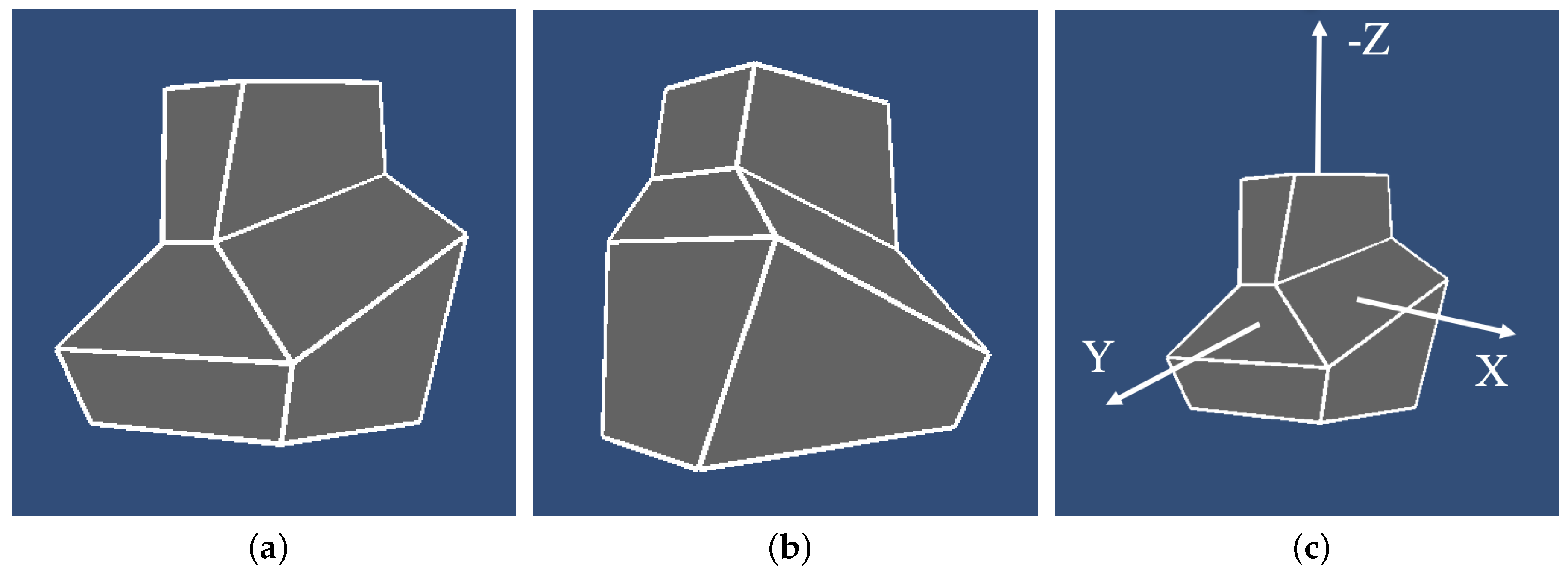
The stimuli were 3D symmetrical polyhedra and 3D asymmetrical polyhedra. The asymmetrical stimuli were created by distorting symmetrical ones. Our symmetrical polyhedra were similar to those used by Li et al. [27]. Two views of one symmetrical shape are shown in Figure 1.
We used abstract shapes to avoid biases, if any, due to familiarity [23,33]. All our shapes had 16 vertices. They can be thought of as consisting of three hexahedrons, with one of the faces of each hexahedron being coplanar with one face of the other two hexahedrons. The symmetry plane of the symmetrical shape was perpendicular to this planar surface of the shape, and the x-axis was the normal of the symmetry plane.
As mentioned earlier, three-dimensional symmetry is a prior used by the human visual system. Li et al. [27] also showed the significance of compactness prior in 3D shape perception of symmetric shapes. In this study, we show how these two priors operate when the 3D shape is not symmetrical. We generated 3D shapes with varying degrees of asymmetry and compactness. To measure asymmetry of a shape, we use a normalized average of absolute difference of corresponding angles. Specifically, consider to be the eight vertices of a symmetrical polyhedron on one side of the symmetry plane. Each of these vertices has a symmetrical counterpart. Let these symmetrical counterparts be represented by . Each subset of 3 vertices from all 16 define three angles depending on their order. For instance, the three vertices , and , define angles (), () and (). For each of these angles, we have its symmetric counterpart. For the three angles mentioned above, the symmetric counterparts are (), () and (), respectively. The number of unique angles is therefore given by . Let these unique angles (in radians) be represented by the ordered set A = {}. We will use the differences between an angle and its symmetric counterpart as a measure of asymmetry. Let the ordered set = {} represent the symmetric counterparts of the angles in set A. The measure of asymmetry can now be defined as:
Note that there are only unique angular differences that can be considered, as we do not need to count each angle twice. Since we are using the absolute value, the above calculation would give us just that. Note that among all unique angles possible, there will be angles that do not represent angles formed by edges of the polyhedron. The division by is to normalize the metric to a number between zero and one. For a perfectly symmetrical shape, the measure will be zero. Our asymmetrical shapes are affine transformations of symmetrical ones. So, even though the asymmetrical shapes do not have a plane of symmetry because they are not symmetrical, we can use a unique “symmetry” correspondence which is the same as the correspondence in the symmetrical shape that was used to produce the asymmetrical one. Perceptually, our asymmetrical shapes do look like distorted symmetrical ones. Therefore, one can refer to our asymmetrical shapes as “near-symmetrical”.
Compactness is computed from the volume V and surface area S of the shape as . After this ratio is normalized to the compactness of a sphere, one gets a number between zero and one, and this number is scale invariant. As mentioned before, we need to have shapes with varying degrees of symmetry and compactness as part of our stimuli. To accomplish this, each 3D shape (stimulus) is classified as belonging to one of the groups shown in Table 1. In the table, and represent asymmetry and compactness measures of the 3D shape, respectively.
We generated two shapes for each of the nine groups. The resulting 18 shapes formed a session in the experiment: 6 symmetrical shapes and 12 asymmetrical shapes. There were five such sessions, with a total of 90 shapes. To generate a stimulus, a random symmetrical shape was first generated and then modified to produce a shape belonging to one of the nine groups. Figure 1c depicts the orientation of the initial symmetrical shape with its symmetry plane orthogonal to the X-axis of the 3D Cartesian coordinate system. The symmetrical shape was aligned so that the planar bottom of the shape was parallel to the XZ-plane. To modify the compactness, the shape was either stretched or compressed along the X- or Z-axes. This process generated shapes belonging to groups 1, 4, and 7. To generate asymmetrical shapes, the original symmetrical shape was repeatedly sheared according to Equation (7) until the desired asymmetry level was obtained.
By stretching/compressing the shape to modify compactness and by shearing the shape to modify asymmetry, stimuli belonging to all nine categories were generated.
Each session had two shapes from each of the nine groups listed in Table 1, one of which was shown to the subjects with the slant of the symmetry plane equal to 45 and the other with the slant of either 20 or 70. Note that asymmetrical shapes do not have any symmetry planes. In those shapes, the slant refers to the YZ-plane, which was the symmetry plane before shearing. The main motivation for using a 45 slant was to have a view that led, in Li et al.’s [27] experiment, to accurate recovery with both monocular and binocular vision. The motivation for using slants of 20 and 70, which are close to degenerate views, was to produce large recovery errors. Once the slant of the shape’s symmetry plane was decided, there was still one degree of freedom in specifying the exact view of the 3D shape, i.e., the shape can still rotate around the normal of the symmetry plane. A random angle of rotation was chosen, subject to two constraints. The first constraint was that at least 10 vertices of the shape needed to be visible, and the second constraint required at least 5 of the 8 vertices forming the “top” of the shape to be visible. These constraints were designed by Li et al. [27] to make sure that the 3D shape can be fully recovered by the human visual system and by the model.
The stimuli were generated using the game engine Unity (known commonly as Unity3D). To display the stimuli, we used Oculus Rift, a virtual reality (VR) head-mounted display. Oculus Rift comes with a head tracker and a joystick. Unity has built-in support for certain VR devices like Oculus Rift. The desired view of the shape can be obtained in Unity by setting the rotation, translation and scaling transformations of the shape appropriately. Unity also allows the use of both orthographic and perspective projections to display the shape. In our experiment, we used perspective projection. The interocular distance can be set in Unity, based on which Unity generates appropriate stereoscopic images for Oculus Rift. We used the head tracker of Oculus to make sure that the head movements of the subject did not change the simulated position of the eyes with respect to the shape being displayed. This means that when the subject moved his head, the shape moved the same way. This is like having the subject’s head on a virtual chin rest. In the actual experiment, the subjects did not move their head a lot.
3.2. Procedure
In the experiment, a stationary reference 3D shape was shown in front of the subject and, on the right, a test adjustable shape was shown rotating. The adjustment involved the three parameters and from Equation (5). The values of these three parameters were chosen randomly at the beginning of each trial. However, these initial random values were confined to the range (–3, 3) for and and to the range (0.1, 3) for . This was done to avoid highly distorted shapes. The subject’s task was to look at the stationary reference shape and adjust the shape of the rotating test shape on the right side of the screen to match the perceived 3D shape of the reference shape. The continuous rotation of the test shape was around Y-axis. In order to make sure that the subjects compared 3D shapes and not 2D images, the test 3D shape was first rotated by 45 around the X-axis before applying the continuous rotation around the Y-axis. This ensured that none of the views of the rotating test shape matched the projection of the reference shape. The adjustment of the three parameters was done using the joystick. The rotating test shape matched, geometrically, the stationary reference 3D shape for the following values: and . The subject was not shown the values of the three parameters during the trial.
In the binocular viewing condition, the reference shape was rendered at a distance of one meter from the subject’s cyclopean eye. In the “monocular” viewing condition, the subject still viewed with both eyes, but the shape was rendered at a distance of one kilometer. Note that the object’s size was proportionally scaled up by a factor of 1000 so that the retinal size of the shape was similar in both viewing conditions. The average angular distance from the centroid of the shape to its vertex was 10.32. The large distance in the “monocular” condition meant that the binocular disparity information available to the subject was negligible. Recall that binocular disparity is inversely proportional to the square of the viewing distance [34].
Each session consisted of 18 trials. Each subject ran a total of 5 monocular and 5 binocular sessions for a total of 90 trials (90 shapes) in monocular viewing and 90 trials in binocular viewing. The same 90 shapes were used in monocular and binocular viewing and all subjects were tested with the same shapes. However, the order in which individual subjects were tested with the five sessions and the order of monocular vs. binocular sessions were randomized. Three subjects were tested, including two of the authors (VJ and ZP). The third subject was naïve about the underlying theory. Each session of 18 trials took around 60–90 min to complete. The subjects were allowed to take breaks at any point of time. Before the actual experiment started, the subjects were given adequate practice sessions until they felt comfortable with the task. In the beginning of each trial, the subject was also asked whether he perceived the shape to be symmetrical or not. Then, the subject adjusted the rotating shape by using three controls of the joystick. Some shapes looked very close to perfectly symmetrical, and so, the subject had to decide whether he called the shape symmetrical or not. In other words, these binary responses might have confounded the percept with response bias. Note, however, that our main analyses that included building computational models ignored these binary responses. These responses were used, however, in some graphs that showed the relation between the shape recovered by the subject and the reference shape, or the shape recovered by the model.
The work was carried out in accordance with the Code of Ethics of the World Medical Association (Declaration of Helsinki). We obtained a written consent from all subjects who participated in the experiments.
4. Model
The data collected from the experiment were used to build models. The emphasis in this paper is on the quality of the fit of the model to human results. This is why we present separate models for monocular and binocular conditions. Within each viewing condition (monocular or binocular), separate models are also considered for symmetric and asymmetric shapes. In the Discussion section, we comment on the possibility of simplifying this approach so that fewer models are used.
Li et al. (2009) showed that, for symmetric shapes viewed monocularly, maximum compactness and minimum surface priors could be used to recover the perceived 3D shape from the 2D image. Specifically, the 3D shape that maximizes the ratio , where V is the volume and S is the surface area of the polyhedron, is very close to what human observers perceive. Therefore, for symmetrical shapes in the monocular condition, we used the same model as the one presented in Li et al. (2009). The ratio will hereafter be referred to as modified compactness. This model has no free parameters.
For asymmetrical shapes in monocular condition, the model consists of a weighted sum of asymmetry and modified compactness. In our experiment, the subject could recover an asymmetrical shape, and therefore, the asymmetry term representing the symmetry prior is explicitly included in the cost function, along with the modified compactness prior used in Li et al. (2009). The cost associated with a shape H is given by:
Here, is the asymmetry measure of shape H, is the modified compactness of shape H, is the weight of the asymmetry term, and is the maximum value of modified compactness that can be achieved by a shape, belonging to the family of shapes, that can be generated from shape H, by applying the 3D affine transformation in Equation (5). The weight decides the importance of the asymmetry relative to modified compactness of the shape. According to the model, the shape which minimizes this cost is the perceived shape. To determine the weight of the asymmetry term, which is the only free parameter, the subject’s data were used. Let the shapes recovered by the subject and the model be referred to as subject shape and model shape, respectively. The idea is to find the weight that minimizes the average shape difference between the subject shape and the model shape. In order to do this, a metric to perform shape comparison is required. The asymmetry metric can be modified to obtain a shape difference metric. To compare two shapes, and , Equation (6) can be used. The set A = {} now represents all the possible angles of shape and the set = {} represents the corresponding angles of shape . Using this shape difference metric, the best weight found for each subject in monocular viewing of asymmetrical shapes is listed in Table 2. An exhaustive search was used to determine the weights.
Note that our shape dissimilarity metric, based on comparing angles, is consistent with the conventional definition of shape, because it is invariant under rigid motion and size scaling. However, we are not claiming that the human visual system uses our formula, but examination of our results strongly suggests that whatever the human visual system uses is likely to be correlated with our measure.
In the binocular condition, for both symmetrical and asymmetrical shapes, the cost function is a weighted sum of asymmetry, binocular depth order and modified compactness. Li et al. [27] established the importance of the depth order cue in 3D shape perception. The asymmetry and modified compactness terms represent the monocular priors, and the binocular depth order term represents the likelihood (or the data term). The depth order score for a shape H is computed as follows. For each pair of visible vertices of shape H, a score is assigned using the function below:
where and are two visible vertices of the shape H, is the absolute value of binocular disparity (in minutes of arc) between the corresponding vertices in the reference 3D shape, = –1 if the two vertices have the same depth order as the corresponding vertices in the reference 3D shape, and = 1 if the depth order of the vertices and is different from that of the reference shape. Once such a score is assigned to each visible pair of vertices, the depth order score for the shape H is computed as:
where represents the set of all unique pairs of visible vertices of shape H, and || represents the number of elements in the set . Equation (9) uses a logistic function to represent visual noise, whereas Li et al. [27] used a cumulative Gaussian distribution function.
The cost function associated with a shape H in the binocular condition is now given by:
where and are the weights of the asymmetry term and depth order terms, respectively. The same cost function is used to model both the symmetrical and asymmetrical cases but with different weights. Data from the experiment were used to estimate the weights. The optimal weights found by exhaustive search for each subject are listed in Table 3. The shape which minimizes this cost function represents the model’s prediction of the perceived 3D shape. Note that the weights for symmetrical shapes in binocular viewing are similar across the three subjects. However, for asymmetrical shapes, there are quite large differences. Li et al. [27] also found some individual differences in binocular viewing: one subject, whose stereoacuity threshold was very high, had binocular performance similar to monocular performance. However, Li et al. only tested symmetrical shapes. As Table 3 shows, our three subjects were all quite similar with symmetrical shapes. It is the asymmetrical shapes that revealed larger individual differences. Specifically, EP’s and ZP’s asymmetry term has weight which is an order of magnitude greater than the weight of the depth order cue, while VJ’s weights for these two terms are similar. Furthermore, VJ’s depth order term has weight greater than the weight of compactness, while ZP’s depth order term has weight smaller than the weight of compactness. It has to be pointed out that one cannot draw any conclusions about the relative importance of the three terms in a cost function by just comparing weights, simply because the three terms are computed using different units. However, one can interpret the relative contribution of the three terms across subjects, as we did just above.
To test the accuracy of the model, we started with a control psychophysical experiment, which is described next.
5. Control Experiment
In the control experiment, the same set of 3D shapes, as used in the experiment described above, were used. The subject was shown a stationary 3D shape in the center and two rotating 3D shapes were shown on the right. One of the rotating shapes was the shape the subject recovered (subject shape) in the main experiment. The other 3D shape was the shape recovered by the model (model shape). The two rotating shapes were shown side by side and the placement of these shapes (left vs. right) was random from trial to trial. The subject was asked to choose the 3D shape from the two rotating 3D shapes which best corresponded to his percept of the stationary 3D shape. The models described above can be considered good models if the subject has chance performance (50/50). Two of the subjects, EP and VJ, participated in the control experiment.
6. Results
The results in Table 4 show that the models described above do a good job in predicting the shape perceived by the subjects because the subject’s performance was not far from chance. This also means that the shape metric which was used to build the models is a good measure of the shape dissimilarity between shapes. The fact that EP chose the model shape in favor of his own shape almost 70% of trials in monocular viewing could be related to the operation of visual and motor noise when the subject was recovering shapes in the main experiment. The easiest way to see evidence of this is to check the data points in Figure 2 representing symmetrical shapes perceived as symmetrical (red diamonds). The asymmetry of the subject shapes is not zero as it should be, since they were judged by the subjects in the beginning of the trial as symmetrical. Our models, on the other hand, did not have any noise except for the finite, but small, steps in the three adjusted parameters when the cost function was minimized. So, if the models are correct, they may recover 3D shapes that match the percept better than the shapes recovered by the subject, himself.
An important observation here is that, in the monocular condition, a simple combination of asymmetry and modified compactness, which are global properties of the shape, can effectively model the abstract shapes that we used. Without using any other priors, the model was able to account for the subject’s percept. In the binocular condition, the only additional information required was the binocular depth order derived from the binocular disparity. Even for shapes which are not perfectly symmetrical (near-symmetrical shapes), combining the binocular depth order information with symmetry and modified compactness priors leads to a good model of shape perception.
We already know that the models are good because they produce shapes that are similar to what the subjects produce. This was shown in the control experiment described just above. This can also be directly seen by examining the 3D shapes on the website (https://lorenz.ecn.purdue.edu/~vthottat/shapeexp/chooseshp.php). Note that the same set of 90 shapes was used, in monocular and binocular viewing, for all three subjects. This allows more direct comparison of one subject to another. The website shows the view that was presented in the psychophysical experiment (in binocular viewing this was one of the two images projected to the left and right eyes). Next to this view we show the actual reference 3D shape presented to the subject, the 3D shape recovered by the subject and the 3D shape recovered by the model. The website contains 540 trials like this (3 subjects × 90 shapes × 2 viewing conditions: monocular and binocular). We do not expect the reader to look through all 540 trials. However, we felt that the reader should have an opportunity to view as many as they wish, because no summary statistics will do justice to what was actually observed. This would also provide the reader with an opportunity to judge the goodness of the models and that of the metrics we used.
We began the quantitative evaluation of the subject’s and model’s recovery with symmetrical shapes. Already, Li et al. [27] showed that this recovery is extremely accurate in binocular vision. However, their subjects dealt with a simpler task, in which all shapes were symmetrical and the only characteristic that was adjusted was the aspect ratio. In our experiment, we used both symmetrical and asymmetrical shapes and the subject adjusted three parameters which allowed them to recover symmetrical or asymmetrical shapes.
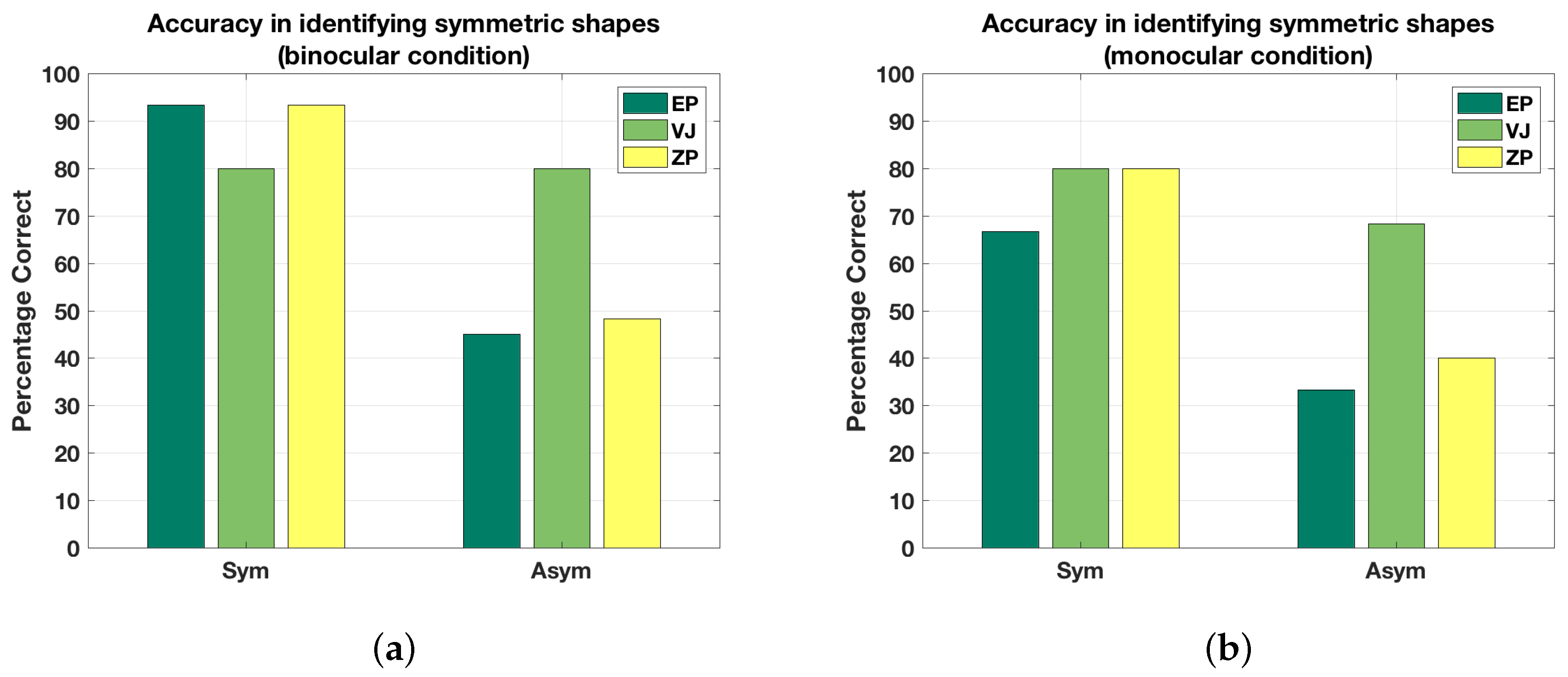
Figure 3 shows the accuracy of identifying symmetrical and asymmetrical shapes correctly in monocular and binocular viewing by the three subjects. This graph is based on the binary responses that the subject produced before performing 3D recovery. Note that we are not computing d’ for this discrimination task, although this in principle could be done. The number of trials is small (30 symmetrical and 60 asymmetrical shapes), so any estimate of d’ would be quite unreliable. The proportion correct on symmetrical and asymmetrical trials, which is what we plotted on Figure 3, is likely affected by response bias. As a result, we will not be drawing any strong conclusions based on these proportions. It can be seen in Figure 3 that symmetrical shapes are almost always (80–95% of the time) identified as symmetrical in binocular viewing. They are also frequently (65–80% of the time) correctly identified as symmetrical in monocular viewing. The differences among the three subjects were pretty small. With asymmetrical shapes, VJ was clearly more correct (by a factor of 2) than the other two subjects. It seems that VJ put more emphasis on the depth order information, as evidenced by the weights in the models. EP and ZP’s binocular percepts, on the other hand, were affected more by compactness and symmetry priors.
These two priors pushed the binocular percept away from the true, asymmetrical reference shape and towards symmetrical and compact shapes. When recovering the shapes, VJ spent twice as much time as EP and ZP. This led to higher precision in recovering the 3D shapes. This will show up in smaller shape dissimilarities between the shapes recovered by VJ and the reference shapes, as compared to these dissimilarities for subjects EP and ZP.
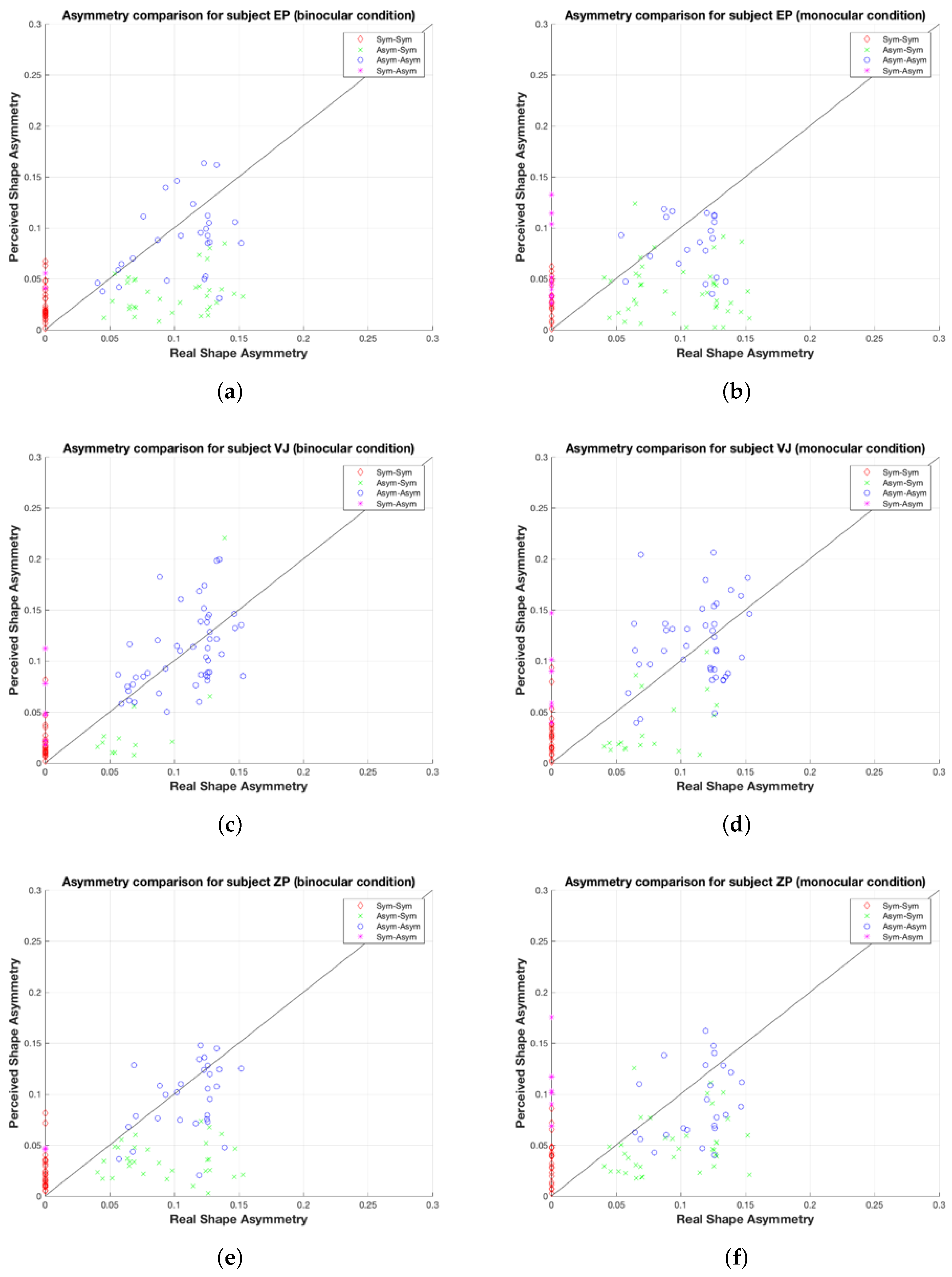
Next, look at Figure 2, which shows scatterplots of perceived shape asymmetry (i.e., asymmetry of the shape recovered by the subject) vs. reference shape asymmetry for four types of trials. The trials have been grouped into four groups based on the binary responses, symmetrical vs. asymmetrical, that were collected in the beginning of each trial. The diagonal line represents the points where perceived shape and reference shape asymmetries are equal. The label ‘Sym-Sym’ indicates symmetrical shapes perceived as symmetrical, ‘Asym-Sym’ indicates asymmetrical shapes perceived as symmetrical, and so on. Red diamonds indicate symmetrical shapes that were classified as symmetrical. It can be seen that the perceived asymmetry of these shapes is not zero. This represents the limited precision of the visual system, as well as limited precision of the motor system. The adjustment task was not easy because the interaction of the three parameters was not intuitively obvious. So, reducing asymmetry of the shape required coordinated change of all three parameters. VJ was the most patient from the three subjects—he also spent most time during the task. Still, most of the symmetrical shapes that were classified as symmetrical resulted in a subject shape with asymmetry not larger than 0.05. Note that a value of 1 for shape asymmetry corresponds to an average difference of 180 ( radians) between corresponding angles in the left and right half of the shape (see Equation (6)). So, a value of 0.05 corresponds, on average, to a 9 difference between corresponding angles. Examination of the 3D shapes on the website shows that the symmetrical shapes were almost always recovered as shapes that were not far from symmetrical.
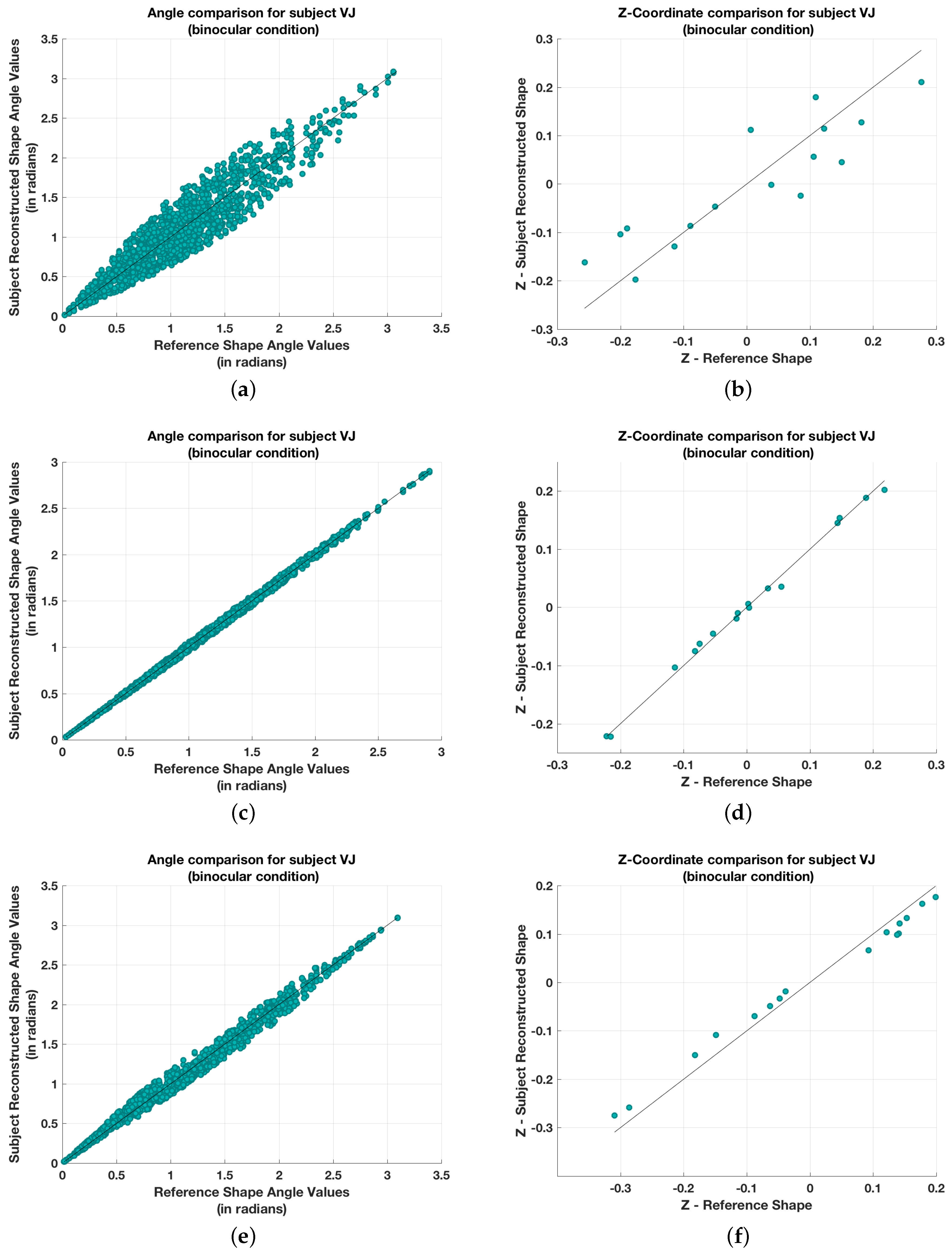
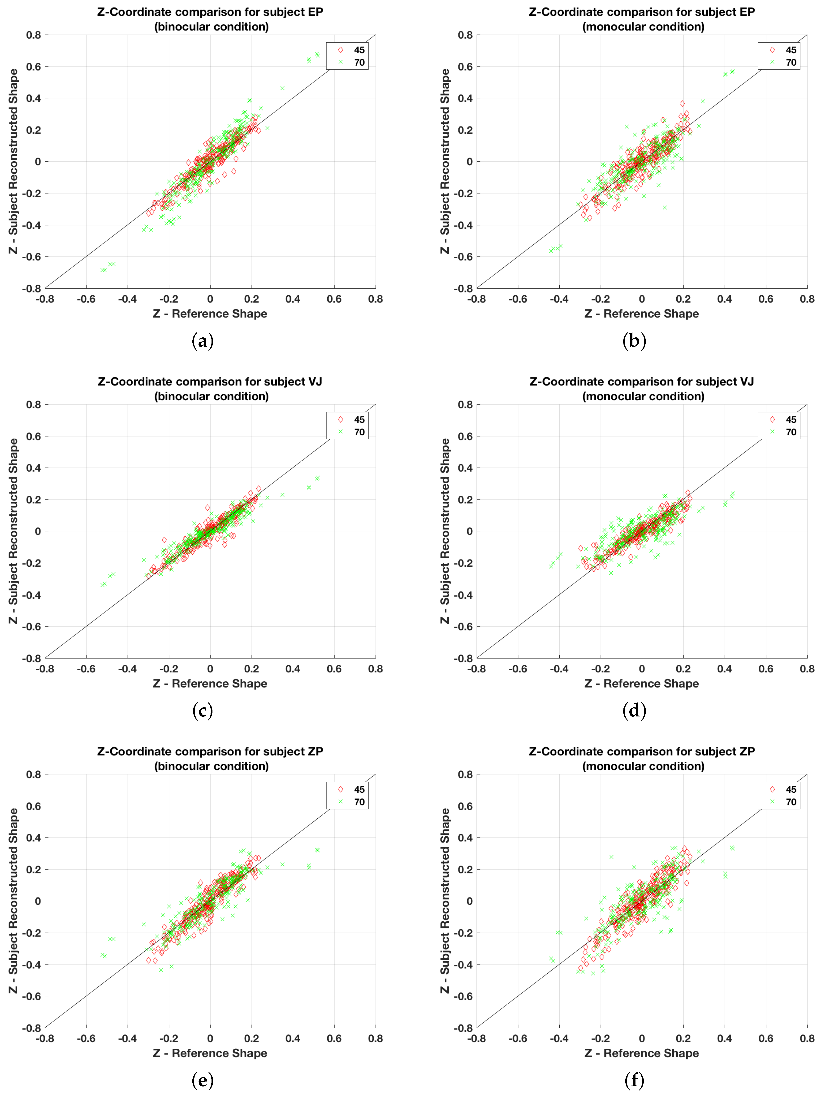
Next, look at Figure 4, left column, which shows the scatterplots illustrating the relation between the angles in the recovered shape and the angles in the reference shape for three symmetrical shapes recovered by VJ in binocular viewing. The first row in Figure 4 shows the plots for the shape in (row = 2, column = 5) in set 2 for subject VJ in binocular viewing on the website. Note that both row and column indices start at one. The second row in Figure 4 represents the shape (row = 2, column = 6) in set 5, and the third row in Figure 4 represents the shape (row = 3, column = 3) in set 3 on the website. These three trials illustrate the range of correlations that we observed. The scatterplot on top shows one of the weakest correlations we observed. Each scatterplot has 16 × 15 × 14/2 data points because we considered all unique angles formed by all triplets of vertices. All scatterplots for symmetrical shapes were within the range shown in Figure 4. The correlation between perceived and actual angles is strong, and all data points are clustered around the diagonal. Figure 4, right column, also shows the analogous scatterplots illustrating the relation between the depths of points in the recovered shape and depths of points in the reference shape for the same three symmetrical shapes viewed binocularly by VJ. These scatterplots have only 16 data points, which is the number of vertices in our 3D shapes. The Z coordinates of the recovered and the reference shapes were taken when the shapes had the same 3D orientation relative to the viewer. More precisely, both 3D shapes, reference and subject, produced the same orthographic image. The fact that all data points are clustered around the diagonal means that there was no systematic distortion of binocularly viewed shapes along the depth direction. This makes sense on rational grounds. Stretching or compressing a 3D symmetrical shape along the depth direction, when the shape is not viewed from perfectly degenerate direction, would have destroyed the symmetry of the 3D shape. Since symmetrical shapes are almost always perceived as symmetrical, there is not much space for depth distortion.
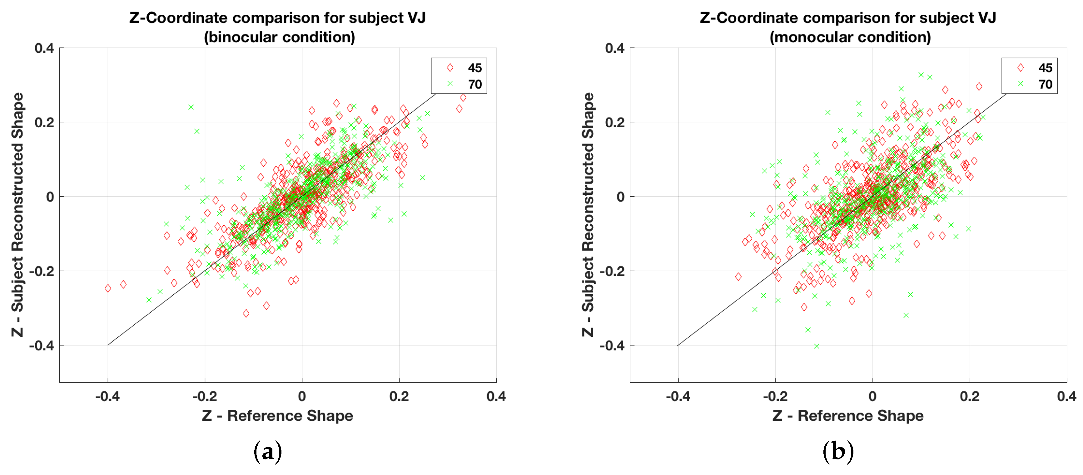
Figure 5 shows scatterplots of the depths of points for all symmetrical shapes for the three subjects for monocular and binocular viewing. Note that in the monocular condition, to ensure that there was no binocular disparity information available, the shapes were displayed at a depth of 1 km after scaling up the shapes by a factor of 1000. In Figure 5 and Figure 6, the Z-coordinate values for the monocular condition is scaled down by a factor of 1000 for better comparison with the binocular condition. It can be seen that all data points in Figure 5, except a few, are close to the diagonal line. This means that there are no systematic distortions of depth: no systematic under- or overestimation. Figure 6 shows analogous graphs for all asymmetrical shapes for subject VJ in monocular and binocular conditions (graphs not shown here, and illustrating the other two subjects are similar). The scatterplots for asymmetrical shapes are substantially noisier in comparison to the corresponding plots for the symmetrical shapes. Notice that the distortion (noise) does not seem to be systematic. The most natural explanation for greater veridicality with symmetrical shapes, as compared to asymmetrical, is the influence of the priors, especially the symmetry prior. The strong effect of a symmetry prior implies that the percept of symmetrical shapes should be more veridical than the percept of asymmetrical ones. This indeed is the case.
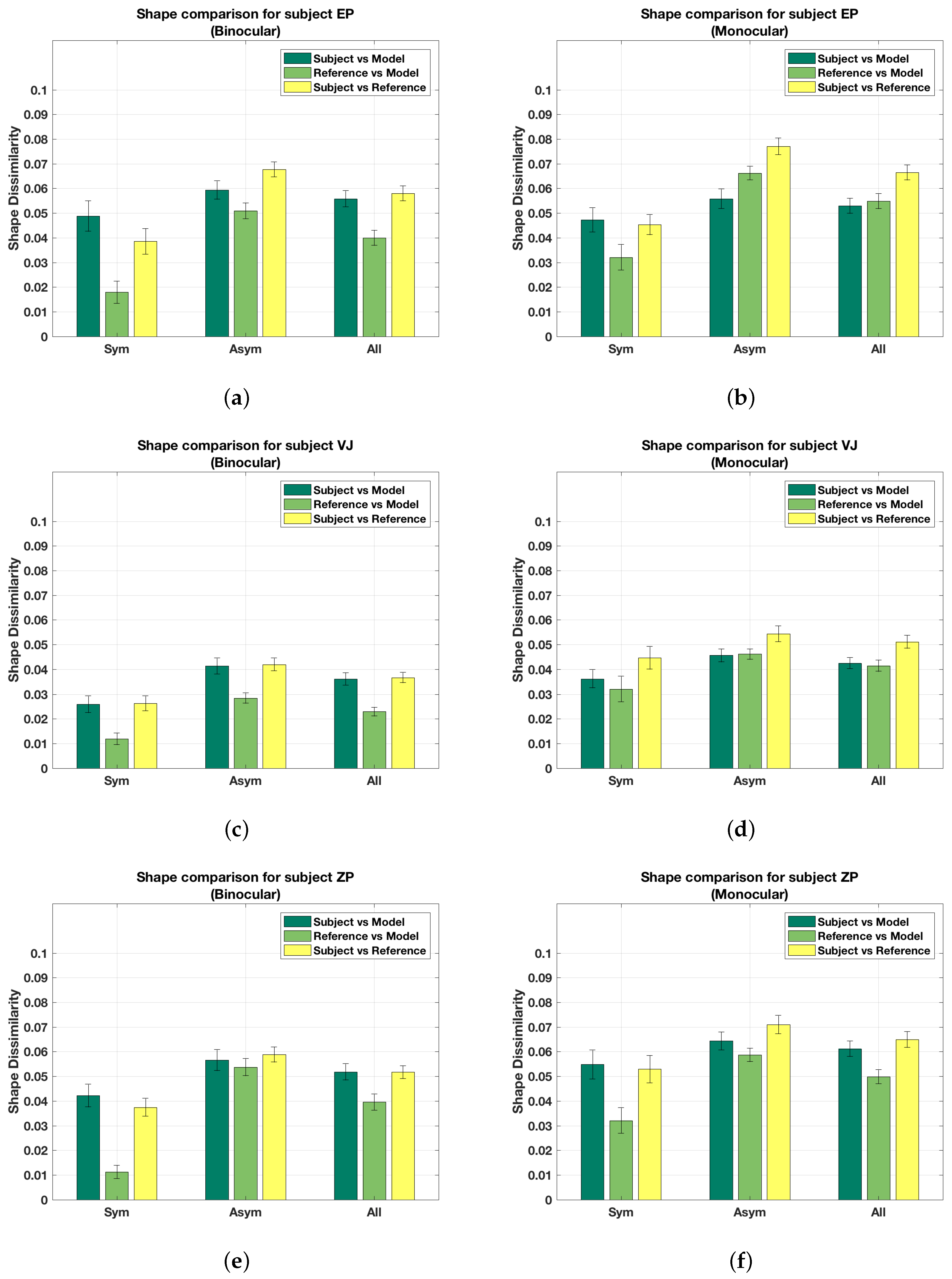
Figure 7 shows shape dissimilarity for all subjects, with the bars grouped into different cases. The label ‘Sym’ represents the average shape dissimilarity for symmetrical shapes. Similarly, ’Asym’ refers to the average shape dissimilarity for asymmetrical shapes. The label ’All’ indicates the average shape difference for all 90 shapes in that condition.
Note that the binocular percept is closer to veridical than the monocular percept is, as can be seen from the subject vs. reference shape dissimilarity values (yellow bar in the group labeled ’All’). Similarly, perception of symmetrical shapes is closer to veridical in comparison to asymmetrical shapes. This can also be verified qualitatively by examining the shapes on the website. Finally, model shapes are closer to the subject shapes than the reference shapes are. This means that, despite small errors between the subject shapes and the reference shapes, the model is a good predictor of what the subjects see.
7. Discussion
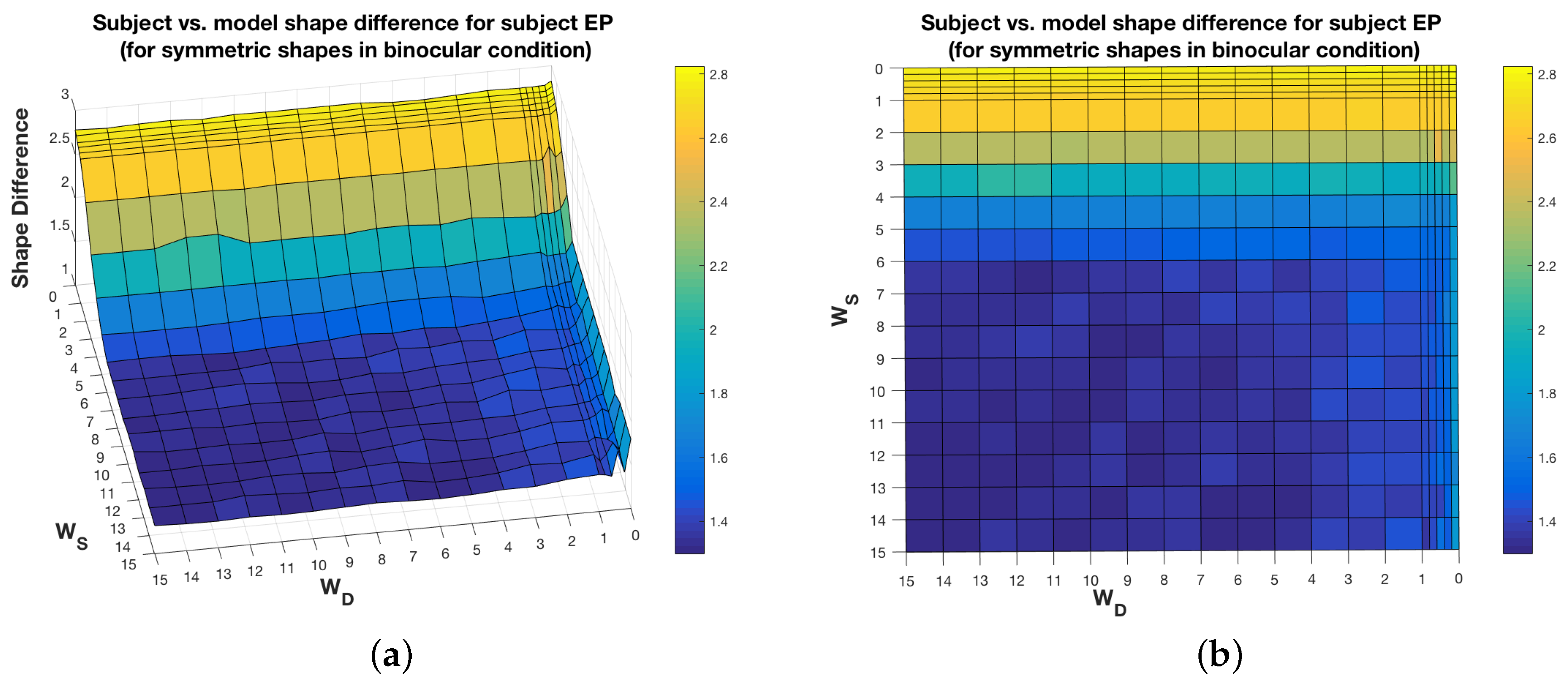
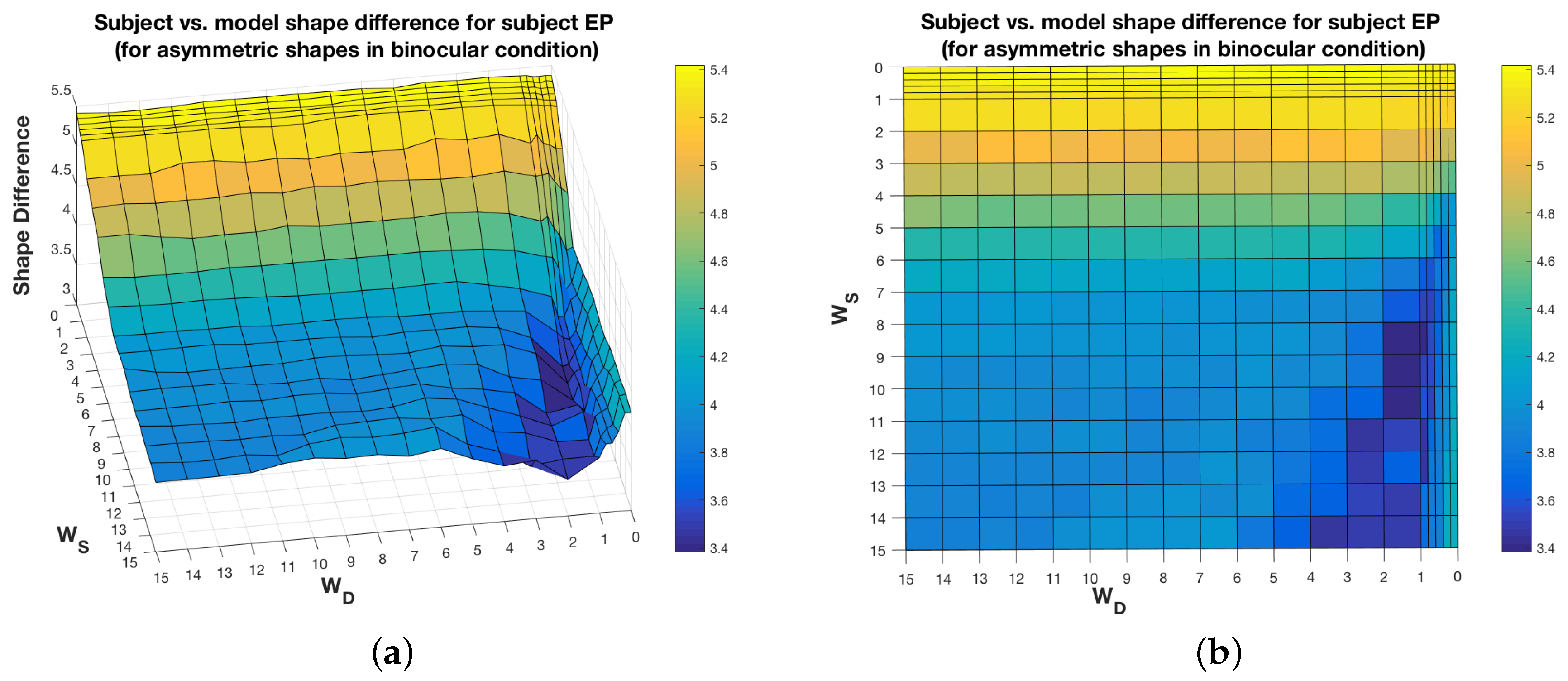
It has to be pointed out that the 3D shape recovery is quite robust to perturbation of the weights around their optimal values. A plot of the shape difference between the shape recovered by the subject and the shape recovered by the model, as a function of the weights of the model, shows that there are other weight values which could be chosen, without increasing the shape difference substantially. As shown in Figure 8, there are flat regions around the optimal weight values for the symmetrical shapes in the case of subject EP in the binocular condition. This is true for the other subjects, too. There are obviously some weight values, like choosing , which would lead to large errors (shape differences), but there is a range of other weight values with errors close to the optimal error. However, for other cases, like for asymmetrical shapes in the binocular condition for subject EP (Figure 9), there seems to be a narrow range of weight values that minimize the error. This is also true for subject ZP but not for subject VJ, i.e., for subject VJ, there are flat regions around the optimal weights, just like in the case of symmetrical shapes. In short, in some cases, there is some flexibility in choosing the weights for a good model. The issue of computational stability of our models in the neighborhood of optimal values of the parameters will be studied in our future work.
Next, it has to be pointed out that, even though different models are used for symmetric objects in monocular and binocular conditions, the relative importance of symmetry in comparison to modified compactness can be the same in both viewing conditions. That is, if we minimize Equation (8), with the weight equal to that of the symmetric case in the binocular condition, the model will produce a shape very close to the one obtained by using the model presented in Li et al. [26]. For instance, the average shape difference between the shape obtained with the model presented in Li et al. [26] and the shape obtained by minimizing Equation (8) with = 7.6 (the optimal weight for subject VJ) is 1.9 × , and the maximum shape difference between the corresponding shapes is 2.3 × . A value of 0.01 for the shape difference metric corresponds to an average difference of between corresponding angles of the two shapes being compared. Therefore, a shape difference metric value of 1.9 × implies an average difference of 3.4 × degrees between corresponding angles of the two shapes. Furthermore, a shape difference metric value of 2.3 × corresponds to an average difference of 4.1 × degrees between corresponding angles of the two shapes. These are extremely small values, and, therefore, the shapes generated by the two models are essentially the same.
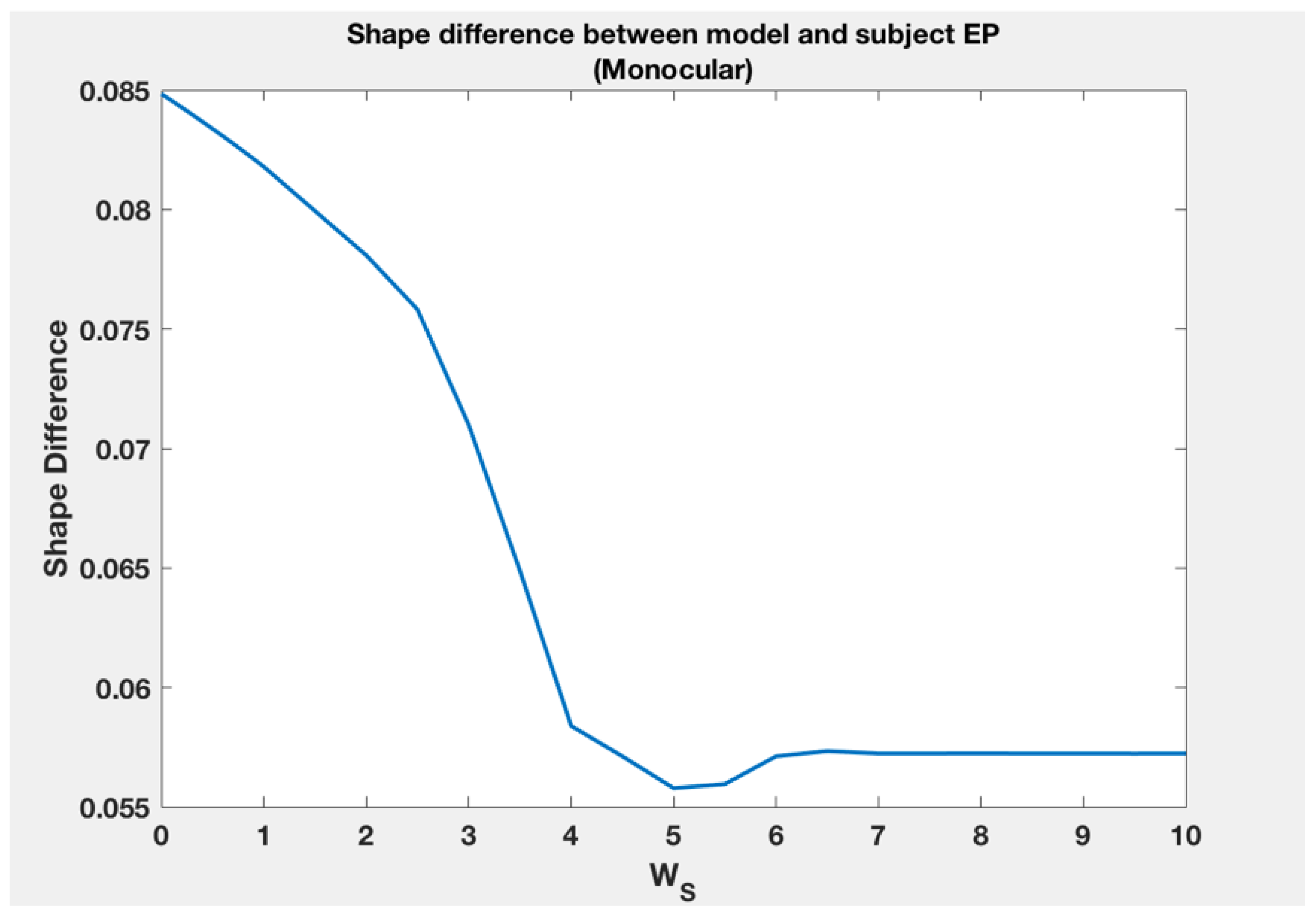
For asymmetrical shapes, the weight of the asymmetry term relative to modified compactness is similar in monocular and binocular conditions for subjects VJ and ZP. For asymmetrical shapes, if the binocular model weights for VJ are used for the monocular model of VJ, the average subject shape vs. model shape difference would go up by 0.0094. Doing the same for subject ZP would lead to an increase in the average shape difference of 0.0022 between the subject and the model. These are not large changes. For asymmetrical shapes for subject EP though, the weight of the asymmetry term seems to be very different across the two conditions. However, as shown in Figure 10, assigning = 10, for asymmetrical shapes in the monocular condition for subject EP, will not lead to any substantial change in shape difference with subject shapes. Therefore, for all three subjects, the weight of asymmetry relative to modified compactness is similar across conditions.
To summarize the above analysis, we do not need separate models for monocular and binocular viewing. However, we need two different binocular models per subject: one for symmetrical shapes and the other for asymmetrical shapes. The monocular model is obtained from either of them by simply dropping the binocular depth order term. In natural viewing, this “dropping” happens naturally when the effectiveness of stereoacuity drops with increasing viewing distance and decreasing object size. Now, how realistic is it to have two different binocular models (cost functions) in the visual system: one for symmetrical and the other for asymmetrical shapes? How does the visual system distinguish between symmetrical and asymmetrical shapes in the first place? If the 3D shape is asymmetrical, the binocular depth order cue can inform the visual system about the asymmetry. For example, once the 3D symmetry correspondence is established in a single 2D retinal image, assuming that the 3D shape is symmetrical (which is always possible—see [35]), stereoacuity can reject this 3D hypothesis. Asymmetrical perception could also result from other biases (priors). For instance, the visual system might prefer an asymmetrical shape with planar faces instead of a symmetrical shape that violates planarity of the faces. Next, given that the importance (weight) of compactness relative to depth order goes up with asymmetrical shapes, compactness could be another factor leading to an asymmetrical percept [29]. We have not done any simulations yet to examine this issue, but it seems reasonable to assume that planarity, compactness and binocular depth order could all be involved when the visual system decides whether to use the cost function for symmetrical shape or asymmetrical shape.
Author Contributions
Conceptualization, V.J., T.S., E.D. and Z.P.; Data curation, V.J. and Z.P.; Formal analysis, V.J.; Funding acquisition, Z.P.; Methodology, V.J., T.S. and Z.P.; Supervision, E.D. and Z.P.; Writing original draft, V.J.; Writing review & editing, V.J., T.S., E.D. and Z.P.
Funding
This research was supported by the National Eye Institute of the National Institutes of Health under award number 1R01EY024666-01.
Conflicts of Interest
The authors declare no conflict of interest.
Appendix A. A 2D Orthographic Image of an Asymmetrical 3D Shape in our Experiment Allows for Recovering 3D Symmetrical Shapes
The XYZ Cartesian coordinate system of a 3D scene and the xy Cartesian coordinate system of a 2D image in the scene are set as follows: (i) the Z-axis of the 3D coordinate system is perpendicular to the image plane and is defined by Z = 0, (ii) the Z-axis passes through the origin of the 2D coordinate system, and (iii) the X- and Y-axes of the 3D coordinate system coincide with the x- and y-axes of the 2D coordinate system, respectively. Under an orthographic projection, a 2D orthographic projection of a point in a 3D scene is = (see Equation (1)).
Assume that a 3D symmetrical shape is given. Its symmetry plane is perpendicular to the image plane and normal to the X-axis. A 3D asymmetrical shape used in this study was generated by deforming the 3D symmetrical shape using a subgroup of 3D affine transformation (see Equation (4)):
where and are positive. This symmetric shape is referred as the “original” symmetric shape for clarity. After this transformation, the original symmetric shape becomes asymmetric unless = 0. After this transformation, the plane, that was a symmetry plane originally, is not normal to its “symmetry” line-segments anymore and they are referred as an “asymmetry plane” and “asymmetry line-segments” after the transformation. The asymmetry line-segments are still parallel to one another and are bisected by the asymmetry plane.
Consider that this asymmetric shape is randomly rotated and is orthographically projected to the image plane along the Z-axis. Assume that the projections of the asymmetry plane and the asymmetry line-segments are “not” degenerate. Namely, the asymmetry plane is not perpendicular to and the asymmetry line-segments are not normal to . If their projections are degenerate, the asymmetry plane is projected to a line in the image and the asymmetry line-segment is projected to a point in the image.
The orientations of the X- and Y-axes of the 3D coordinate system and of the x- and y-axes of the 2D coordinate system are reset so that the X- and x-axes are parallel with orthographic projections of the asymmetry line-segments. Then, an orientation of the asymmetry line-segments can be represented by a vector . Consider two vectors and that are parallel to the asymmetry plane.
A subject is asked to choose a 3D shape from a subgroup of 3D affine transform of the asymmetric shape in the experiment. The subgroup of 3D affine transform is controlled by three parameters and is represented by a matrix :
where and are positive real numbers that the subject can adjust. The vectors , and are transformed by into and , respectively. Note that the orthographic image of the asymmetric shape on is an invariant of . The images of the asymmetry line segments stay parallel to the X-axis under .
In the rest of Appendix A, we show there is always some 3D symmetric shape that can be obtained by transforming the asymmetric shape by . Symmetry line-segments and a symmetry plane of this symmetric shape are transformed from the asymmetry line-segments and the asymmetry plane of the asymmetric shape. Namely, and are parallel to the symmetry plane, is parallel to the symmetry line-segments, is perpendicular to and is normal to the symmetry plane. Note that the asymmetric shape is in the subgroup of 3D affine transform (Equation (A1)) of the original symmetric shape, and Equation (A2) is another subgroup of 3D affine transform. Hence, the asymmetry line-segments still connect pairs of points that were symmetrical pairs of the original symmetric shape. The asymmetry line-segments are still parallel to one another and are bisected by the asymmetry plane, but the asymmetry line-segments are not normal to the symmetry plane. Hence, transforms the asymmetrical shape into a symmetrical shape if is perpendicular to and .
Recall that the images of the asymmetry line-segments are parallel to the X-axis. Under this condition, the symmetry plane of the symmetrical shape transformed from the asymmetric shape is perpendicular to the ZX-plane [29,31]. The Y-axis is parallel to .
and is perpendicular to and . Then, the orientation of the symmetry plane can be determined by its slant from the Z-axis. The slant of the symmetry plane can be defined as an angle between the Z-axis and the normal to the symmetry plane:
Recall that and are perpendicular to one another and is perpendicular to the Y-axis. Hence,
From Equations (A3), (A4) and (A5), for transforming the asymmetric shape into the symmetric shape can be derived as follows:
where . Such exists unless = . If , the asymmetric line-segments are parallel to the asymmetry plane (Note that = only if the asymmetrical shape is planar because of the process generating the asymmetrical shape in this study. The asymmetrical shape was generated by transforming the original 3D symmetrical shape with a subgroup of 3D affine transformation (Equation (A1)). The asymmetry line-segments and the asymmetry plane are transformed from symmetry line-segments and a symmetry plane of the original shape. The symmetry line-segments are normal to the symmetry plane, and 3D affine transformation can make them parallel only by compressing the original symmetrical shape along some orientation until the shape becomes planar.) Equation (A6) shows there is a one-parameter family of 3D symmetric shapes that can be transformed from the asymmetric shape. The family can be controlled by the slant of the symmetry plane. These symmetric and asymmetric shapes can be projected to the identical image.
References
- Hochberg, J.; McAlister, E. A quantitative approach, to figural “goodness”. J. Exp. Psychol. 1953, 46, 361. [Google Scholar] [CrossRef] [PubMed]
- Wallach, H.; O’connell, D. The kinetic depth effect. J. Exp. Psychol. 1953, 45, 205–217. [Google Scholar] [CrossRef] [PubMed]
- Hay, J.C. Optical motions and space perception: An extension of Gibson’s analysis. Psychol. Rev. 1966, 73, 550. [Google Scholar] [CrossRef] [PubMed]
- Ullman, S. The interpretation of structure from motion. Proc. R. Soc. Lond. B 1979, 203, 405–426. [Google Scholar] [CrossRef] [PubMed] [Green Version]
- Longuet-Higgins, H.C. A computer algorithm for reconstructing a scene from two projections. Nature 1981, 293, 133–135. [Google Scholar] [CrossRef]
- Kopfermann, H. Psychologische untersuchungen über die wirkung zweidimensionaler darstellungen körperlicher Gebilde. Psychol. Forsch. 1930, 13, 293–364. [Google Scholar] [CrossRef]
- Perkins, D.N. How good a bet is good form? Percept. 1976, 5, 393–406. [Google Scholar] [CrossRef] [PubMed]
- Witkin, A.P. Recovering surface shape and orientation from texture. Artif. Intell. 1981, 17, 17–45. [Google Scholar] [CrossRef]
- Brady, M.; Yuille, A. Inferring 3D orientation from 2D contour (an extremum principle). In Natural Computation; MIT Press: Cambridge, MA, USA, 1983. [Google Scholar]
- Sugihara, K. Machine Interpretation of Line Drawings; MIT Press: Cambridge, MA, USA, 1986; Volume 2. [Google Scholar]
- Marill, T. Emulating the human interpretation of line-drawings as three-dimensional objects. Int. J. Comput. Vis. 1991, 6, 147–161. [Google Scholar] [CrossRef]
- Leclerc, Y.G.; Fischler, M.A. An optimization-based approach to the interpretation of single line drawings as 3D wire frames. Int. J. Comput. Vis. 1992, 9, 113–136. [Google Scholar] [CrossRef] [Green Version]
- Poggio, T.; Torre, V.; Koch, C. Computational vision and regularization theory. Nature 1985, 317, 314–319. [Google Scholar] [CrossRef] [PubMed]
- Pizlo, Z.; Rosenfeld, A.; Weiss, I. The geometry of visual space: About the incompatibility between science and mathematics. Comput. Vis. Image Understand. 1997, 65, 425–433. [Google Scholar] [CrossRef]
- Pizlo, Z. Perception viewed as an inverse problem. Vis. Res. 2001, 41, 3145–3161. [Google Scholar] [CrossRef]
- Sawada, T.; Pizlo, Z. Detection of skewed symmetry. J. Vis. 2008, 8, 14. [Google Scholar] [CrossRef] [PubMed]
- Wagemans, J. Characteristics and models of human symmetry detection. Trends Cogn. Sci. 1997, 1, 346–352. [Google Scholar] [CrossRef] [Green Version]
- Makin, A.D.; Rampone, G.; Bertamini, M. Conditions for view invariance in the neural response to visual symmetry. Psychophysiology 2015, 52, 532–543. [Google Scholar] [CrossRef] [PubMed]
- Saunders, J.A.; Knill, D.C. Perception of 3D surface orientation from skew symmetry. Vis. Res. 2001, 41, 3163–3183. [Google Scholar] [CrossRef] [Green Version]
- Van der Vloed, G.; Csatho, A.; van der Helm, P.A. Symmetry and repetition in perspective. Acta Psychol. 2005, 120, 74–92. [Google Scholar] [CrossRef] [PubMed]
- Steiner, G. Spiegelsymmetrie der Tierkörper. Naturwiss. Rundsch. 1979, 32, 481–485. [Google Scholar]
- Rock, I.; DiVita, J. A case of viewer-centered object perception. Cogn. Psychol. 1987, 19, 280–293. [Google Scholar] [CrossRef]
- Pizlo, Z.; Stevenson, A.K. Shape constancy from novel views. Percept. Psychophys. 1999, 61, 1299–1307. [Google Scholar] [CrossRef] [PubMed] [Green Version]
- Li, Y.; Pizlo, Z. Depth cues versus the simplicity principle in 3D shape perception. Top. Cogn. Sci. 2011, 3, 667–685. [Google Scholar] [CrossRef] [PubMed]
- Biederman, I.; Gerhardstein, P.C. Recognizing depth-rotated objects: Evidence and conditions for three-dimensional viewpoint invariance. J. Exp. Psychol.-Hum. Percep. Perf. 1993, 19, 1162. [Google Scholar] [CrossRef]
- Li, Y.; Pizlo, Z.; Steinman, R.M. A computational model that recovers the 3D shape of an object from a single 2D retinal representation. Vis. Res. 2009, 49, 979–991. [Google Scholar] [CrossRef] [PubMed]
- Li, Y.; Sawada, T.; Shi, Y.; Kwon, T.; Pizlo, Z. A Bayesian model of binocular perception of 3D mirror symmetrical polyhedra. J. Vis. 2011, 11, 11. [Google Scholar] [CrossRef] [PubMed]
- Vetter, T.; Poggio, T. Symmetric 3D objects are an easy case for 2D object recognition. Spat. Vis. 1994, 8, 443–453. [Google Scholar] [CrossRef] [PubMed]
- Sawada, T. Visual detection of symmetry of 3D shapes. J. Vis. 2010, 10, 4. [Google Scholar] [CrossRef] [PubMed]
- Pizlo, Z.; Li, Y.; Sawada, T.; Steinman, R. Making a Machine that Sees Like Us; Oxford University Press: New York, NY, USA, 2014. [Google Scholar]
- Pizlo, Z.; Sawada, T.; Li, Y.; Kropatsch, W.G.; Steinman, R.M. New approach to the perception of 3D shape based on veridicality, complexity, symmetry and volume. Vis. Res. 2010, 50, 1–11. [Google Scholar] [CrossRef] [PubMed] [Green Version]
- Todd, J.T.; Bressan, P. The perception of 3-dimensional affine structure from minimal apparent motion sequences. Percep. Psychophys. 1990, 48, 419–430. [Google Scholar] [CrossRef] [Green Version]
- Chan, M.W.; Stevenson, A.K.; Li, Y.; Pizlo, Z. Binocular shape constancy from novel views: The role of a priori constraints. Atten. Percep. Psychophys. 2006, 68, 1124–1139. [Google Scholar] [CrossRef] [Green Version]
- Howard, I.; Rogers, B. Seeing in Depth: Depth Perception; Oxford University Press: New York, NY, USA, 2008; Volume 2. [Google Scholar]
- Sawada, T.; Li, Y.; Pizlo, Z. Any pair of 2D curves is consistent with a 3D symmetric interpretation. Symmetry 2011, 3, 365–388. [Google Scholar] [CrossRef]
Figure 1.
An example of a symmetrical polyhedron. The “top” of the shape is shown in (a), (b) shows the flat (planar) “bottom” of the shape and (c) shows the shape’s coordinate system.
Figure 1.
An example of a symmetrical polyhedron. The “top” of the shape is shown in (a), (b) shows the flat (planar) “bottom” of the shape and (c) shows the shape’s coordinate system.

Figure 2.
Perceived vs. real asymmetry of shapes for (a) subject EP (binocular); (b) subject EP (monocular); (c) subject VJ (binocular); (d) subject VJ (monocular); (e) subject ZP (binocular) and (f) subject ZP (monocular).
Figure 2.
Perceived vs. real asymmetry of shapes for (a) subject EP (binocular); (b) subject EP (monocular); (c) subject VJ (binocular); (d) subject VJ (monocular); (e) subject ZP (binocular) and (f) subject ZP (monocular).

Figure 3.
Accuracy in identifying symmetrical and asymmetrical shapes in (a) binocular and (b) monocular condition. Recall that there were 30 symmetrical and 60 asymmetrical shapes.
Figure 3.
Accuracy in identifying symmetrical and asymmetrical shapes in (a) binocular and (b) monocular condition. Recall that there were 30 symmetrical and 60 asymmetrical shapes.

Figure 4.
Perceived vs. real angles (first column, in radians) and depth (second column) for three different symmetric shapes. Each row represents the corresponding plots for a particular shape. (a) and (b) represent the plots for the shape in (row = 2, column = 5) in set 2; (c) and (d) represent the plots for the shape in (row = 2, column = 6) in set 5 and (e) and (f) represent the plots for the shape in (row = 3, column = 3) in set 3 on the https://lorenz.ecn.purdue.edu/~vthottat/shapeexp/chooseshp.php.

Figure 5.
Subject shape vs. reference shape depth plots for symmetrical shapes for (a) subject EP (binocular); (b) subject EP (monocular); (c) subject VJ (binocular); (d) subject VJ (monocular); (e) subject ZP (binocular) and (f) subject ZP (monocular). The numbers 45 and 70 indicate viewing directions. The green x marks include both 20 and 70 viewing directions.

Figure 6.
Perceived vs. real depth plots for asymmetric shapes for subject VJ in (a) binocular and (b) monocular condition.
Figure 6.
Perceived vs. real depth plots for asymmetric shapes for subject VJ in (a) binocular and (b) monocular condition.

Figure 7.
Shape dissimilarity for (a) subject EP (binocular); (b) subject EP (monocular); (c) subject VJ (binocular); (d) subject VJ (monocular); (e) subject ZP (binocular) and (f) subject ZP (monocular).
Figure 7.
Shape dissimilarity for (a) subject EP (binocular); (b) subject EP (monocular); (c) subject VJ (binocular); (d) subject VJ (monocular); (e) subject ZP (binocular) and (f) subject ZP (monocular).

Figure 8.
Subject vs. model shape difference, as function of the model weights, for symmetrical shapes, for the subject EP, in the binocular condition. (a) and (b) represent two views of the same shape difference plot.
Figure 8.
Subject vs. model shape difference, as function of the model weights, for symmetrical shapes, for the subject EP, in the binocular condition. (a) and (b) represent two views of the same shape difference plot.

Figure 9.
Two views ((a) and (b)) of the subject vs. model shape difference, as function of the model weights, for asymmetrical shapes, for the subject EP, in the binocular condition.
Figure 9.
Two views ((a) and (b)) of the subject vs. model shape difference, as function of the model weights, for asymmetrical shapes, for the subject EP, in the binocular condition.

Figure 10.
Shape difference for asymmetric shapes in the monocular condition as a function of the weight of the symmetry term.
Figure 10.
Shape difference for asymmetric shapes in the monocular condition as a function of the weight of the symmetry term.


Table 1.
Asymmetry and compactness of the 3D shapes.
| Symmetry | = 0. 00 | 0.01 < < 0.11 | > 0.11 | |
|---|---|---|---|---|
| Compactness | ||||
| > 0.38 | Group 1 | Group 2 | Group 3 | |
| 0.2 < < 0.38 | Group 4 | Group 5 | Group 6 | |
| < 0.20 | Group 7 | Group 8 | Group 9 | |
Table 2.
Weights for the asymmetry term in the monocular condition.
| Subject | |
|---|---|
| EP | 5.1 |
| VJ | 3 |
| ZP | 4 |
Table 3.
Weights for shapes in the binocular condition.
| Subject | (Symmetrical Case) | (Symmetrical Case) | (Asymmetrical Case) | (Asymmetrical Case) |
|---|---|---|---|---|
| EP | 9.7 | 8.6 | 10 | 1 |
| VJ | 7.6 | 11.5 | 4 | 5.8 |
| ZP | 9.0 | 14.0 | 5 | 0.3 |
Table 4.
Results from the control experiment.
| Subject | Condition | Number of times (out of 90) the model shape was chosen |
|---|---|---|
| EP | Monocular | 62 (68.8%) |
| EP | Binocular | 48 (53.3%) |
| VJ | Monocular | 40 (44.4%) |
| VJ | Binocular | 46 (51.1%) |
© 2018 by the authors. Licensee MDPI, Basel, Switzerland. This article is an open access article distributed under the terms and conditions of the Creative Commons Attribution (CC BY) license (http://creativecommons.org/licenses/by/4.0/).
Share and Cite
MDPI and ACS Style
Jayadevan, V.; Sawada, T.; Delp, E.; Pizlo, Z. Perception of 3D Symmetrical and Nearly Symmetrical Shapes. Symmetry 2018, 10, 344. https://doi.org/10.3390/sym10080344
AMA Style
Jayadevan V, Sawada T, Delp E, Pizlo Z. Perception of 3D Symmetrical and Nearly Symmetrical Shapes. Symmetry. 2018; 10(8):344. https://doi.org/10.3390/sym10080344
Chicago/Turabian StyleJayadevan, Vijai, Tadamasa Sawada, Edward Delp, and Zygmunt Pizlo. 2018. "Perception of 3D Symmetrical and Nearly Symmetrical Shapes" Symmetry 10, no. 8: 344. https://doi.org/10.3390/sym10080344
Note that from the first issue of 2016, this journal uses article numbers instead of page numbers. See further details here.