A Neutrosophic Set Based Fault Diagnosis Method Based on Multi-Stage Fault Template Data

Abstract

Fault diagnosis is an important issue in various fields and aims to detect and identify the faults of systems, products, and processes. The cause of a fault is complicated due to the uncertainty of the actual environment. Nevertheless, it is difficult to consider uncertain factors adequately with many traditional methods. In addition, the same fault may show multiple features and the same feature might be caused by different faults. In this paper, a neutrosophic set based fault diagnosis method based on multi-stage fault template data is proposed to solve this problem. For an unknown fault sample whose fault type is unknown and needs to be diagnosed, the neutrosophic set based on multi-stage fault template data is generated, and then the generated neutrosophic set is fused via the simplified neutrosophic weighted averaging (SNWA) operator. Afterwards, the fault diagnosis results can be determined by the application of defuzzification method for a defuzzying neutrosophic set. Most kinds of uncertain problems in the process of fault diagnosis, including uncertain information and inconsistent information, could be handled well with the integration of multi-stage fault template data and the neutrosophic set. Finally, the practicality and effectiveness of the proposed method are demonstrated via an illustrative example.

1. Introduction

Fault diagnosis aims to identify and repair faults in systems, products, and processes, and has been widely applied to various fields, for instance, military [1,2], economic [3,4], and medicine [5,6], and plays a significant part in the prevention of accidents during the normal operation of equipment [7,8]. Owing to the complexity and uncertainty of the actual environment, fault information is usually imprecise, incomplete, and uncertain, and it is thus, difficult to cope with [9,10,11,12]. The challenge is to devise a fault diagnosis process to reduce the impact of such imprecision, incompletion, and uncertainty as much as possible. Furthermore, the fault information obtained from multiple sources may be different or even conflicting [13]. In such cases, it is important to check conflicts between the information and to aggregate the information into consistent information.

A great deal of research work has been performed in the field of fault diagnosis, some of which has resulted in the application of efficient approaches to exactly and expeditiously diagnose certain types of faults. Nevertheless, most of these methods fail to diagnose multiple types of faults [14,15,16]. To solve this problem, some methods based on Bayes theory were proposed [17,18,19], though efficient aggregation results could only be obtained when the proper and qualified a priori and conditional probabilities were obtainable in the methods based on Bayes theory [20]. As a development of the Bayes theory, the Depmster–Shafer evidence theory was proposed to deal with uncertainty problems [21,22,23,24]. Reference [25] describes the integration of the fuzzy set theory and evidence theory to improve the accuracy of various diagnoses. In addition, there have been several research works based on the use of acoustic signals [26,27,28] for the fault diagnosis of rotating machines. Lee et al. [29] presented a power transformer fault diagnosis method based on set pair analysis (SPA) and association rules. He et al. [30] proposed a novel fault diagnosis method based on the relevance vector machine (RVM) to deal with small data samples. Vibration signal-based fault diagnosis methods [31,32,33] have also proposed in recent years.

However, uncertain factors in the process of fault diagnosis have not been well handled. In order to deal with uncertain problems under fuzzy information and incoherent information, Smarandache defined the concept of a neutrosophic set [34,35,36,37], which is a set of elements that exist in a non-standard unit interval, such as the realness degree, uncertainty degree, or false degree, as a summarization of concepts of the classic set [38], fuzzy set (FS) [39], intuitionistic fuzzy set (IFS) [40,41] and interval valued intuitionistic fuzzy set (IVIFS) [42]. To facilitate the application of the neutrosophic set to practical problems, Wang et al. [43] proposed the concepts of the interval neutrosophic set (INS) and single valued neutrosophic set (SVNS), and Ye [44] defined the concept of the simplified neutrosophic set (SNS). In order to fuse the neutrosophic information to solve realistic problems under a neutrosophic environment, some researchers proposed neutrosophic aggregation operators. For instance, Liu and Wang [45] introduced a single-valued neutrosophic normalised weighted Bonferroni mean operator based on the SVNS. Furthermore, Peng et al. [46] developed simplified neutrosophic information aggregation operators, such as the simplified neutrosophic weighted averaging (SNWA) operator and the simplified neutrosophic weighted geometric (SNWG) operator.

Several methods based on the neutrosophic set have been proposed for fault diagnosis. For instance, Ye proposed cotangent similarity measures for SVNSs based on a cotangent function for the fault diagnosis of steam turbines [47] and the dimension root similarity measure of SVNSs for the fault diagnosis of hydraulic turbines [48], which are all used for fault diagnosis under a single-valued neutrosophic environment. Kong et al. proposed the misfire fault diagnosis method for the fault diagnosis of gasoline engines [49]. Zhang et al. proposed a single-valued neutrosophic (SVN) multi-granulation rough set over a two universe model for the diagnosis of steam turbine faults [50].

There is still a requirement to deal with the uncertainty, imprecision, and incompletion of information and to improve the accuracy of fault diagnosis results with reduced calculations [51,52,53]. Nevertheless, the complex relationships among fault types and various features of faults in fault diagnosis problems leads to difficulty in fault diagnosis. In addition, with changes in time, the unsteadiness of the actual environment causes uncertainty in fault template data collected at different stages. The uncertainty of multi-stage fault template data, however, fails to be dealt with well. In order to solve this problem, a neutrosophic set based fault diagnosis method based on multi-stage fault template data is proposed in this paper. An unknown fault sample whose fault type is unknown is diagnosed by generating its neutrosophic sets based on multi-stage fault template data, and then the SNWA operator is applied to fuse the multi-stage neutrosophic sets of the unknown fault sample under each feature and to fuse the neutrosophic sets of all features of the unknown fault sample again. Afterward, the fault diagnosis results are determined by the application of the defuzzification method to defuzzy the neutrosophic set of each fault type. This proposed method has several main traits. Firstly, in comparison to some traditional fault methods, for instance, the method based on the relevance vector machine [30], the multi-stage fault template data can deal with the uncertainty of collected data due to the unsteadiness of the actual environment. Afterwards, compared with the method based on random fuzzy variables [54], the application of the neutrosophic set gives consideration to the uncertainty of the fault types and the unknown fault sample, which reflects and handles the uncertainty of fault information well. Compared with former neutrosophic set based methods for fault diagnosis [47,48,49,50], the generation of a neutrosophic set based on multi-stage fault template data in this paper can deal with uncertain information better and diagnose the faults efficiently.

The rest of this paper is arranged as follows: Section 2 briefly introduces the concepts of the neutrosophic set, SNS, and the SNWA operator. The proposed method for fault diagnosis is listed step by step in Section 3. In Section 4, a numerical example is used to demonstrate the reasonableness of this proposed method, and to interpret the proposed method. Some summary remarks are shown in Section 5.

2. Preliminaries

The neutrosophic set, introduced by Smarandache [34], is an extension of the classical FS [39], IFS [40], and IVIFS [42]. It is an efficient tool for dealing with the problem with uncertain information. The neutrosophic set concept is defined as follows [43]:

Definition 1.

Let X be a space of points (objects), with a generic element in X denoted by x. A neutrosophic set (A) in X is characterized by a truth-membership function ($T_A$), an indeterminacy-membership function ($I_A$) and a falsity-membership function $(F_A)$. $T_A\left(x\right)$, $I_A\left(x\right)$, and $F_A\left(x\right)$ are real standard or non-standard subsets of $]0^{-},1^{+}[$. That is,

$$\begin{array}{c}{T}_A:X\mapsto ]0^{-},1^{+}[\hfill \\ I_A:X\mapsto ]0^{-},1^{+}[\hfill \\ F_A:X\mapsto ]0^{-},1^{+}[.\hfill \end{array}$$

(1)

There is no restriction on the sum of $T_A\left(x\right)$, $I_A\left(x\right)$ and $F_A\left(x\right)$, so $0^{-}\le sup{T}_A\left(x\right)+sup{I}_A\left(x\right)+sup{F}_A\left(x\right)\le 3^{+}$.

In order to promote the application of the neutrosophic set in practical problems, the notion of SNS [44] was proposed as a subclass of the neutrosophic set. The definition of SNS is as follows [44]:

Definition 2.

Let X be a space of points, with a generic element in X denoted by x. A neutrosophic set (A) in X is characterized by a truth-membership function ($T_A\left(x\right)$), a indeterminacy-membership function ($I_A\left(x\right)$) and a falsity-membership function ($F_A\left(x\right)$). If $T_A\left(x\right):X\to [0,1]$, $I_A\left(x\right):X\to [0,1]$ and $F_A\left(x\right):X\to [0,1]$ satisfied:

$$\begin{array}{c}x\in X\mapsto T_A\left(x\right)\in [0,1]\hfill \\ x\in X\mapsto I_A\left(x\right)\in [0,1]\hfill \\ x\in X\mapsto F_A\left(x\right)\in [0,1]and\hfill \\ 0\le T_A\left(x\right)+I_A\left(x\right)+F_A\left(x\right)\le 3.\hfill \end{array}$$

(2)

Then an SNS A in X can be denoted as

$$A=\left\{\langle x,T_A\left(x\right),I_A\left(x\right),F_A\left(x\right)\rangle \right|x\in X\}$$

(3)

Which is called an SNS. In particular, if X includes only one element, $N=\langle T_A\left(x\right),I_A\left(x\right),F_A\left(x\right)\rangle$ is called a SNN and is denoted by $\alpha =\langle \mu ,\pi ,\nu \rangle$. The numbers $\mu ,\pi ,\nu$ denote, respectively, the degree of membership, the degree of indeterminacy-membership, and the degree of non-membership.

For any two SNSs ($A=\langle T_A\left(x\right),I_A\left(x\right),F_A\left(x\right)\rangle ,B=\langle T_B\left(x\right),I_B\left(x\right),F_B\left(x\right)\rangle$), the operational relations are defined as the following [44]:

$$\begin{array}{c}A+B=\langle T_A\left(x\right)+T_B\left(x\right)-T_A\left(x\right)T_B\left(x\right),I_A\left(x\right)+I_B\left(x\right)-I_A\left(x\right)I_B\left(x\right),F_A\left(x\right)+F_B\left(x\right)-F_A\left(x\right)F_B\left(x\right)\rangle ,\hfill \\ A\times B=\langle T_A\left(x\right)T_B\left(x\right),I_A\left(x\right)I_B\left(x\right),F_A\left(x\right)F_B\left(x\right)\rangle ,\hfill \\ \lambda A=\langle 1-{(1-T_A\left(x\right))}^{\lambda },1-{(1-I_A\left(x\right))}^{\lambda },1-{(1-F_A\left(x\right))}^{\lambda }\rangle ,\lambda >0,\hfill \\ A^{\lambda }=\langle T_A{\left(x\right)}^{\lambda },T_A{\left(x\right)}^{\lambda },T_A{\left(x\right)}^{\lambda }\rangle ,\lambda >0.\hfill \end{array}$$

(4)

Peng et al. [46] developed some simplified neutrosophic information aggregation operators, such as the SNWA operator, which is based on the conception of SNS. It is defined as follows [46]:

Definition 3.

Let ${\alpha }_i=\langle {\mu }_i,{\pi }_i,{\nu }_i\rangle ,i=1,2,\dots ,n$ be a collection of SNNs. Then,

$$\begin{array}{c}SNWA({\alpha }_1,{\alpha }_2,\dots ,{\alpha }_n)=w_1{\alpha }_1+w_2{\alpha }_2+\dots +w_n{\alpha }_n\hfill \\ =\langle 1-\prod _{i=1}^n{(1-{\mu }_i)}^{w_i},\prod _{i=1}^n{\left({\pi }_i\right)}^{w_i},\prod _{i=1}^n{\left({\nu }_i\right)}^{w_i}\rangle ,i=1,2,\dots ,n.\hfill \end{array}$$

(5)

where $w={(w_1,w_2,\dots ,w_n)}^T$ is the weight vector of ${\alpha }_i(i=1,2,\dots ,n)$, with $w_i\in [0,1]$ and ${\displaystyle \sum _{i=1}^n}{w}_i=1$.

3. The Proposed Method

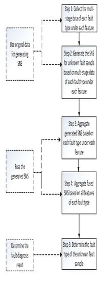
The characteristics of the actual environment in which a system, product, or process is used, for instance, the temperature, location and air, are unstable over time in the fault diagnosis process, even if the equipment works under the same conditions normally, which leads to uncertainty in the data collected at different stages. These factors have obvious impacts on fault diagnosis results. Thus, the uncertainty of fault information must be dealt with to achieve more efficient diagnosis results. In the face of this problem, a neutrosophic set based fault diagnosis method based on multi-stage fault template data is proposed to diagnose the unknown fault sample in this paper. Consider an unknown fault sample (S) with n features ($C=\{C_1,C_2,\dots ,C_n\}$), whose data have been collected under each feature. The aim of this fault diagnosis method is to identify the fault type of the unknown fault sample (S). The flow-process diagram of the proposed method is shown in Figure 1, and the detailed procedures are elaborated step by step in the following text.

Step 1

Collect the multi-stage data of fault types under each feature. Suppose that there are m fault types ($F=\{F_1,F_2,\dots ,F_m\}$) with n features ($C=\{C_1,C_2,\dots ,C_n\}$). Firstly, collect the multi-stage data of each fault type under each feature. Each stage’s data for each fault type under each feature are obtained by continuously collecting within the time interval (T). Suppose that data from k stages of every fault type under every feature are obtained. The multi-stage data of each fault type under each feature are shown as follows:

$$\begin{array}{cc}& \begin{array}{ccccccccccccc}\hfill & & \cdots & & & C_j& & & \cdots & & & & \end{array}\\ \begin{array}{c}\\ ⋮\\ \\ F_i\\ \\ ⋮\\ \end{array}& \left[\begin{array}{ccc}\ddots & ⋮& \ddots \\ \ddots & kstagesdataof{F}_{i}under{C}_j& \ddots \\ \ddots & ⋮& \ddots \end{array}\right]\end{array}$$

where $i=1,2,\dots ,m$ and $j=1,2,\dots ,n$.

Step 2

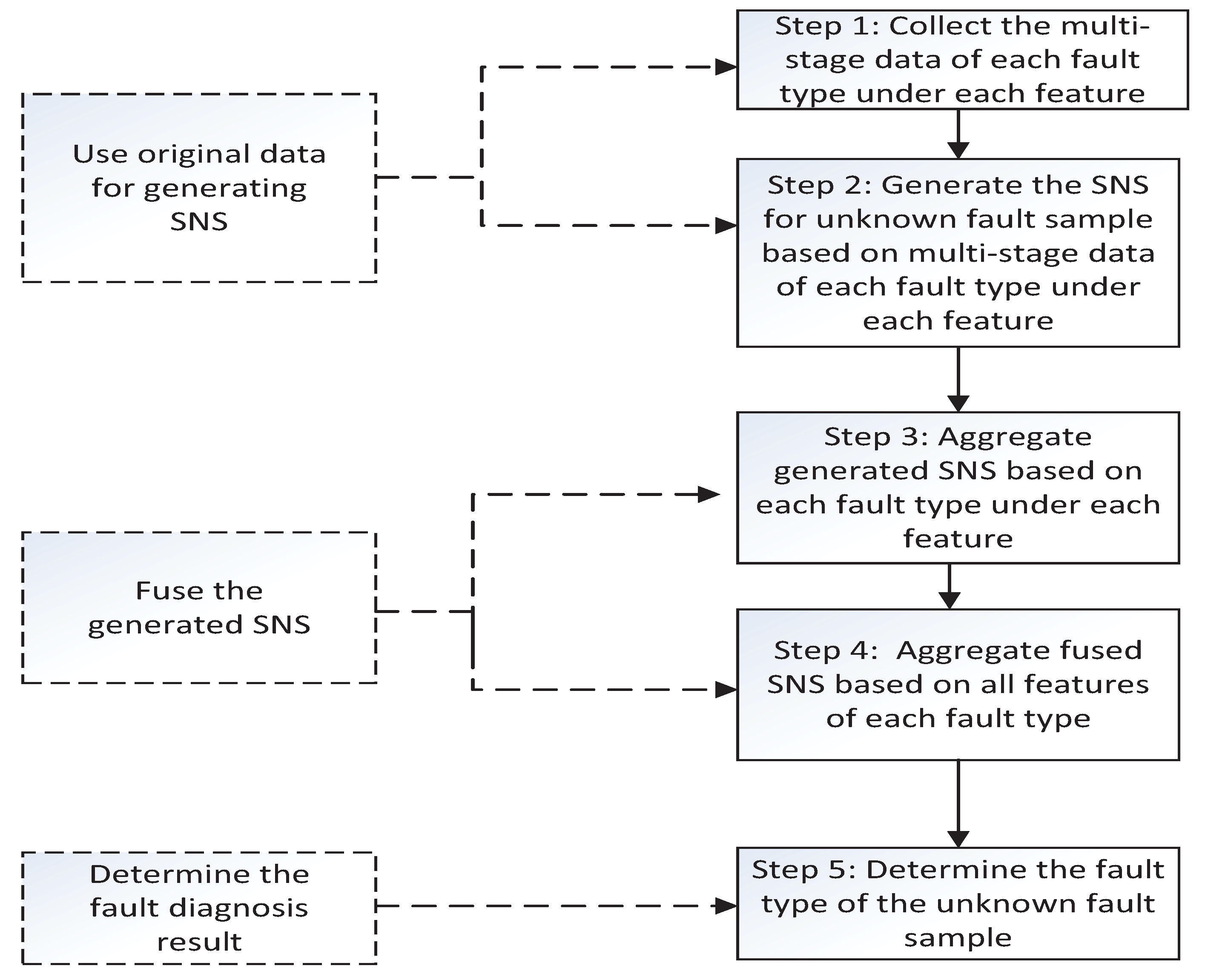
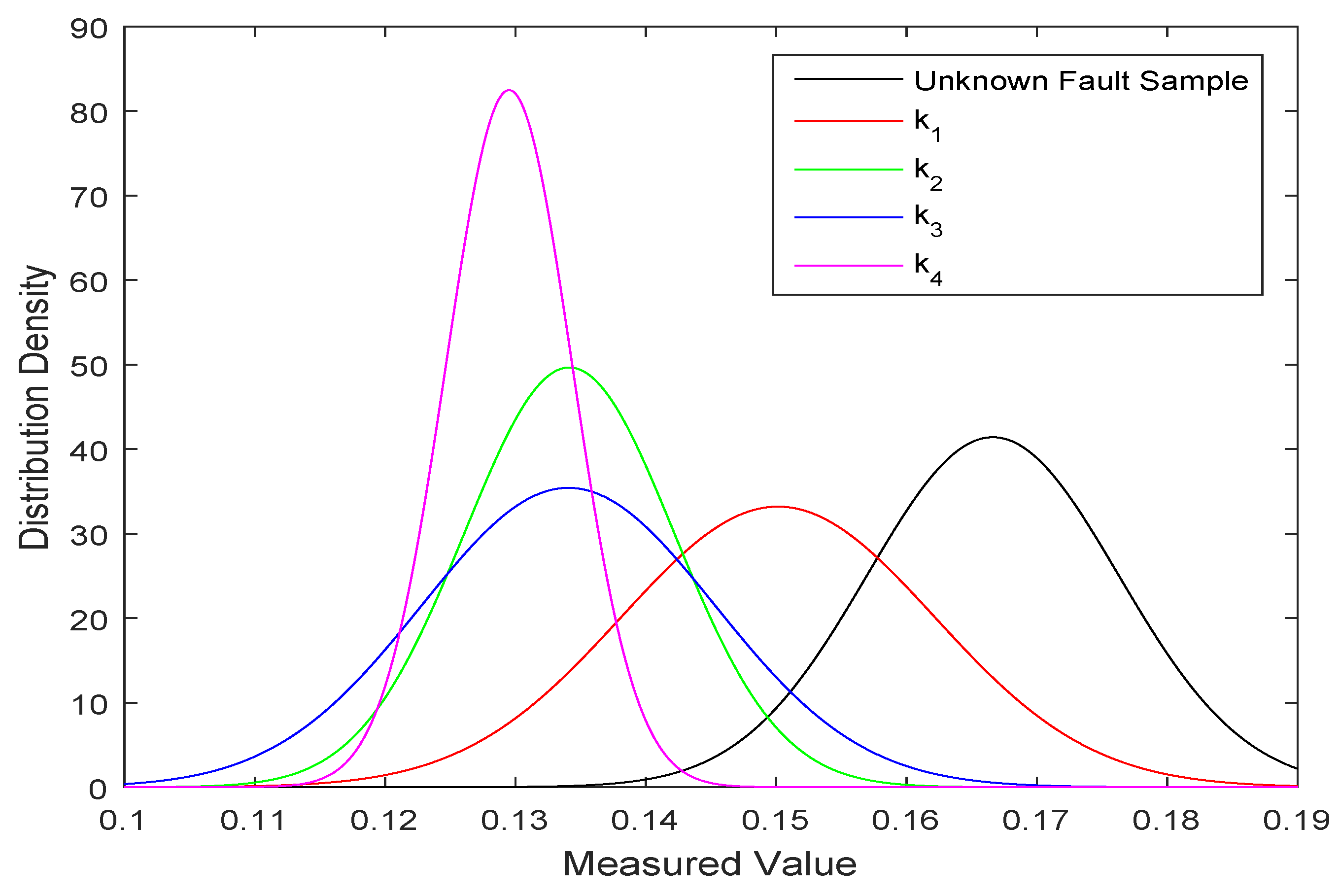
Generate the SNS for an unknown fault sample (S) based on the multi-stage data of each fault type under each feature. For each stage’s data for each fault type under every feature, and for the data of every feature of the unknown fault sample (S), a normal distribution model is established which is obtained by using the arithmetic average (m) and variance (${\sigma }^2$) of a stage’s data as the arithmetic average and standard deviation of the normal distribution model, denoted as $N(m,{\sigma }^2)$. Then, k normal distribution models and k normal distribution figures are generated according to k stages of data of each fault type under each feature. In addition, a normal distribution model is generated based on the data of the unknown fault sample under each feature. The normal distribution figures generated from the data of $C_j$ of unknown fault sample S and k stages of data for $C_j$ of $F_i$ are shown in Figure 2. As the figure shows, each stage’s data collected drift to a certain extent in a certain range. In particular, there are distinct differences between the fault type’s data collected in the fourth stage and the data of the unknown fault sample.

The normal distribution function indicates the distribution probability density of the data. The membership degree of SNS is defined as the ratio of the maximum value of the vertical coordinate of the intersection point between the unknown fault sample and the fault type and the peak value of the unknown fault sample. The two normal distribution curves (Figure 3) and the definition of the membership degree ($\mu$) are as follows:

$$\mu =\frac{y_h}{y_m},$$

(6)

where $y_h$ represents the maximum value of the vertical coordinate of the intersection point of distribution between the unknown fault sample (S) and the fault type ($F_i$), and $y_m$ represents the peak value of the unknown fault sample’s distribution.

As the figure shown, the intersection points of distribution between the unknown fault sample and $F_i$ are marked with X, and the peak point of S’ distribution is marked with X in the same way. Then, from the Equation (6), the membership degree is generated.

In this paper, it is assumed that the non-membership degree and the membership degree are interdependent. The indeterminacy-membership degree indicates the uncertainty degree of neutrosophic information. Entropy represents the uncertainty of the information and has been widely used in many fields. Shannon introduced the quantitative and qualitative model of communication as a statistical process that underlies information theory [55], which is a formalism that was originally applied to digital communication. The indeterminacy-membership degree and non-membership degree are defined as follows:

$$\begin{array}{c}\left(1\right)\nu =1-\mu ,\hfill \\ \left(2\right)\pi =\mu lo{g}_2(\frac{1}{\mu })+\nu lo{g}_2(\frac{1}{\nu }),\mu \ne 0,\nu \ne 0.\hfill \end{array}$$

(7)

The indeterminacy-membership degree ($\pi$) represents the Shannon entropy of the membership degree ($\mu$) and the non-membership degree ($\nu$), and $\pi$ equals 0 if $\mu$ or $\nu$ equal 0. Hence, the SNS can be obtained. The generated SNS is shown in

Table 1. The generated simplified neutrosophic set (SNS) for S based on multi-stage data.

Fault Type	Stage	Feature
		${\mathit{C}}_1$	${\mathit{C}}_2$	⋯	${\mathit{C}}_{\mathit{n}}$
$F_1$	1	$({\mu }_{11}^1,{\pi }_{11}^1,{\nu }_{11}^1)$	$({\mu }_{12}^1,{\pi }_{12}^1,{\nu }_{12}^1)$	⋯	$({\mu }_{1n}^1,{\pi }_{1n}^1,{\nu }_{1n}^1)$
	2	$({\mu }_{11}^2,{\pi }_{11}^2,{\nu }_{11}^2)$	$({\mu }_{12}^2,{\pi }_{12}^2,{\nu }_{12}^2)$	⋯	$({\mu }_{1n}^2,{\pi }_{1n}^2,{\nu }_{1n}^2)$
	⋮	⋮	⋮	⋱	⋮
	k	$({\mu }_{11}^k,{\pi }_{11}^k,{\nu }_{11}^k)$	$({\mu }_{12}^k,{\pi }_{12}^k,{\nu }_{12}^k)$	⋯	$({\mu }_{1n}^k,{\pi }_{1n}^k,{\nu }_{1n}^k)$
$F_2$	1	$({\mu }_{21}^1,{\pi }_{21}^1,{\nu }_{21}^1)$	$({\mu }_{22}^1,{\pi }_{22}^1,{\nu }_{22}^1)$	⋯	$({\mu }_{2n}^1,{\pi }_{2n}^1,{\nu }_{2n}^1)$
	2	$({\mu }_{21}^2,{\pi }_{21}^2,{\nu }_{21}^2)$	$({\mu }_{22}^2,{\pi }_{22}^2,{\nu }_{22}^2)$	⋯	$({\mu }_{2n}^2,{\pi }_{2n}^2,{\nu }_{2n}^2)$
	⋮	⋮	⋮	⋱	⋮
	k	$({\mu }_{21}^k,{\pi }_{21}^k,{\nu }_{21}^k)$	$({\mu }_{22}^k,{\pi }_{22}^k,{\nu }_{22}^k)$	⋯	$({\mu }_{2n}^k,{\pi }_{2n}^k,{\nu }_{2n}^k)$
⋮	⋮	⋮	⋮	⋱	⋮
$F_m$	1	$({\mu }_{m1}^1,{\pi }_{m1}^1,{\nu }_{m1}^1)$	$({\mu }_{m2}^1,{\pi }_{m2}^1,{\nu }_{m2}^1)$	⋯	$({\mu }_{mn}^1,{\pi }_{mn}^1,{\nu }_{mn}^1)$
	2	$({\mu }_{m1}^2,{\pi }_{m1}^2,{\nu }_{m1}^2)$	$({\mu }_{m2}^2,{\pi }_{m2}^2,{\nu }_{m2}^2)$	⋯	$({\mu }_{mn}^2,{\pi }_{mn}^2,{\nu }_{mn}^2)$
	⋮	⋮	⋮	⋱	⋮
	k	$({\mu }_{m1}^k,{\pi }_{m1}^k,{\nu }_{m1}^k)$	$({\mu }_{m2}^k,{\pi }_{m2}^k,{\nu }_{m2}^k)$	⋯	$({\mu }_{mn}^k,{\pi }_{mn}^k,{\nu }_{mn}^k)$

:

Step 3

Aggregate the generated SNS based on each fault type under each feature. In this paper, it is assumed that the weights of data from k stages collected under the same working conditions are equal. The k SNNs of each fault type under each feature are fused via the SNWA operator, as shown in Equation (5). For instance,

$${\alpha }_{11}=SNWA({\alpha }_{11}^1,{\alpha }_{11}^2,\dots ,{\alpha }_{11}^k).$$

(8)

Then, the fused SNS matrix (A) is as follows:

$$A=\begin{array}{cc}& \begin{array}{ccccccccc}\hfill & \cdots & & & C_j& & & \cdots & \end{array}\\ \begin{array}{c}\\ ⋮\\ \\ F_i\\ \\ ⋮\\ \end{array}& \left[\begin{array}{ccc}\ddots & ⋮& \ddots \\ \ddots & ({\mu }_{ij},{\pi }_{ij},{\nu }_{ij})& \ddots \\ \ddots & ⋮& \ddots \end{array}\right]\end{array}$$

where $i=1,2,\dots ,m$ and $j=1,2,\dots ,n$.

Step 4

Aggregate the fused SNS based on all features of each fault type. If the weights of n features are equal, n SNNs of each fault type are fused via the SNWA operator, as shown in Equation (5). For instance,

$${\alpha }_1=SNWA({\alpha }_{11},{\alpha }_{12},\dots ,{\alpha }_{1n}).$$

(9)

Then, the fused SNS matrix (F) is as follows:

$$F=\begin{array}{cc}\begin{array}{c}{F}_1\\ F_2\\ ⋮\\ F_m\end{array}& \left[\begin{array}{c}({\mu }_1,{\pi }_1,{\nu }_1)\\ ({\mu }_2,{\pi }_2,{\nu }_2)\\ ⋮\\ ({\mu }_m,{\pi }_m,{\nu }_m)\end{array}\right].\end{array}$$

Step 5

Determine the fault type of the unknown fault sample. Considering the fuzziness of the unknown fault sample and the fault types, direct application of the defuzzification method can intuitively reflect the results of the fault diagnosis and reduce the amount of calculation in the process of fault diagnosis. The crisp number of each SNN is defuzzied and calculated as follows [56]:

$$C_i={\mu }_i+\left({\pi }_i\right)\left(\frac{{\mu }_i}{{\mu }_i+{\nu }_i}\right).$$

(10)

$C_i$ is the degree to which the information extracted from the data of untested fault supports each fault type. As a result, the ranking order of all the fault types can be determined according to the descending order of their crisp numbers ($C_i$).

4. Illustrative Example and Discussion

In this section, an example of a motor rotor is used to demonstrate the validity and accuracy rate of the proposed method.

The experimental equipment is a multi-functional flexible rotor test-bed. The vibration displacement sensor and acceleration sensor were placed in the horizontal and vertical directions of the rotor support pedestal, respectively, to collect the rotor vibration signals, and the signals were transmitted to the upper computer through the acquisition box. Then, using the data analysis software under the $LabVIEW$ environment, the vibration acceleration spectrum of the rotor and the average amplitude of vibration displacement in the time domain were obtained as the fault feature signals. An unknown fault sample, $S_1$, was used. When the rotor was running normally, the amplitude of each vibration frequency did not exceed 0.1 m/s${}^2$. When the fault occurred, the frequency and augmentation of the amplitudes of different faults were distinct. The vibration energy of three kinds of fault types were mostly concentrated at $1-3X$. Therefore, $S_1$ was determined to have four features:

• $C_1$: The vibration amplitude when the acceleration frequency of the rotor is the basic frequency, $1X$.
• $C_2$: The vibration amplitude when the acceleration frequency of the rotor is the frequency $2X$.
• $C_3$: The vibration amplitude when the acceleration frequency of the rotor is the frequency $3X$.
• $C_4$: The average amplitude of vibration displacement in the time-domain.

The data in this paper originated from ref. [57]. The data of $S_1$ under each feature was collected. For instance, the data of $S_1$ under $C_1$ was as follows:

$$\begin{array}{c}{S_1}_{C_1}Data=[0.14210.14260.14220.14220.14230.14330.1440.14390.14370.1436\hfill \\ 0.14320.14340.14370.14280.14240.14270.14310.14250.14280.1421\hfill \\ 0.14240.1420.14220.14260.14310.14280.14260.14240.14220.1416\hfill \\ 0.14240.14290.14240.14230.14210.1420.1420.14230.14250.1426].\hfill \end{array}$$

Step 1

Collect the multi-stage data of each fault type under each feature. There are three fault types set up on the test-bed:

• $F_1$: Rotor imbalance.
• $F_2$: Rotor misalignment.
• $F_3$: Support base loosening.

For each feature of each fault type, data from five stages were collected, and for each stage’s data, forty consecutive observation values were collected continuously within a time interval of 16 s. The data in this paper originated from Reference [57]. For instance, the first stage’s data of $F_1$ under $C_1$ was as follows:

$$\begin{array}{c}{F_1}_{C_1}FirstStag{e}^{\prime }sData=[0.16630.15900.15680.14850.17230.20060.1903\hfill \\ 0.19080.19860.18430.17850.16100.15790.15110.15320.16470.16280.1646\hfill \\ 0.16340.16420.16480.16400.16740.06610.16590.16500.16330.16320.1604\hfill \\ 0.15420.15550.15620.15400.15640.15570.15420.15460.15710.15370.1536].\hfill \end{array}$$

Step 2

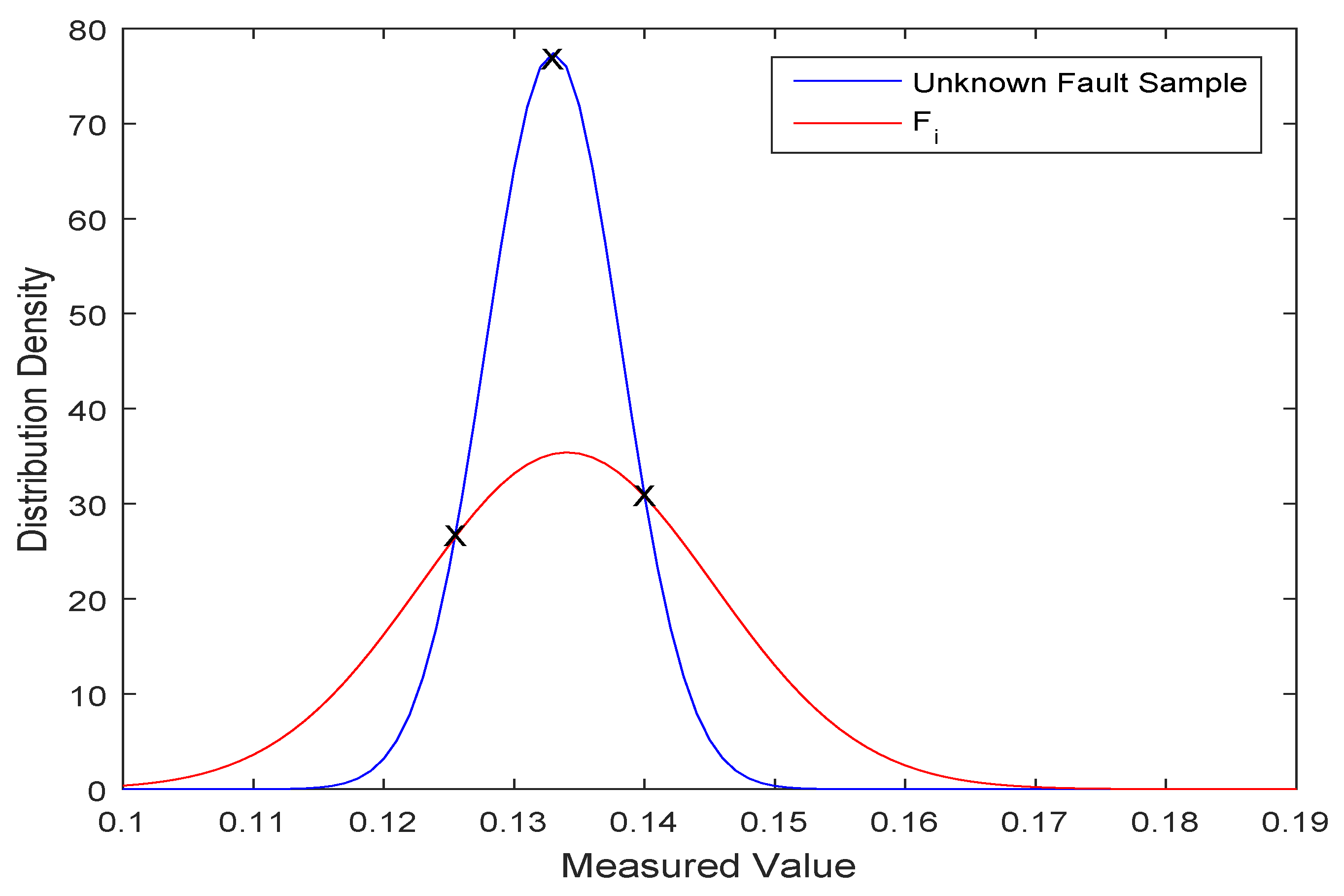
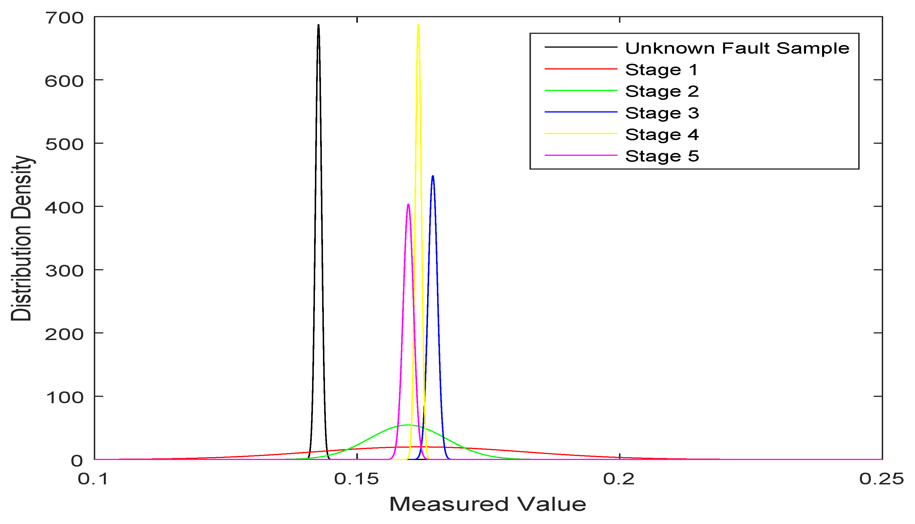
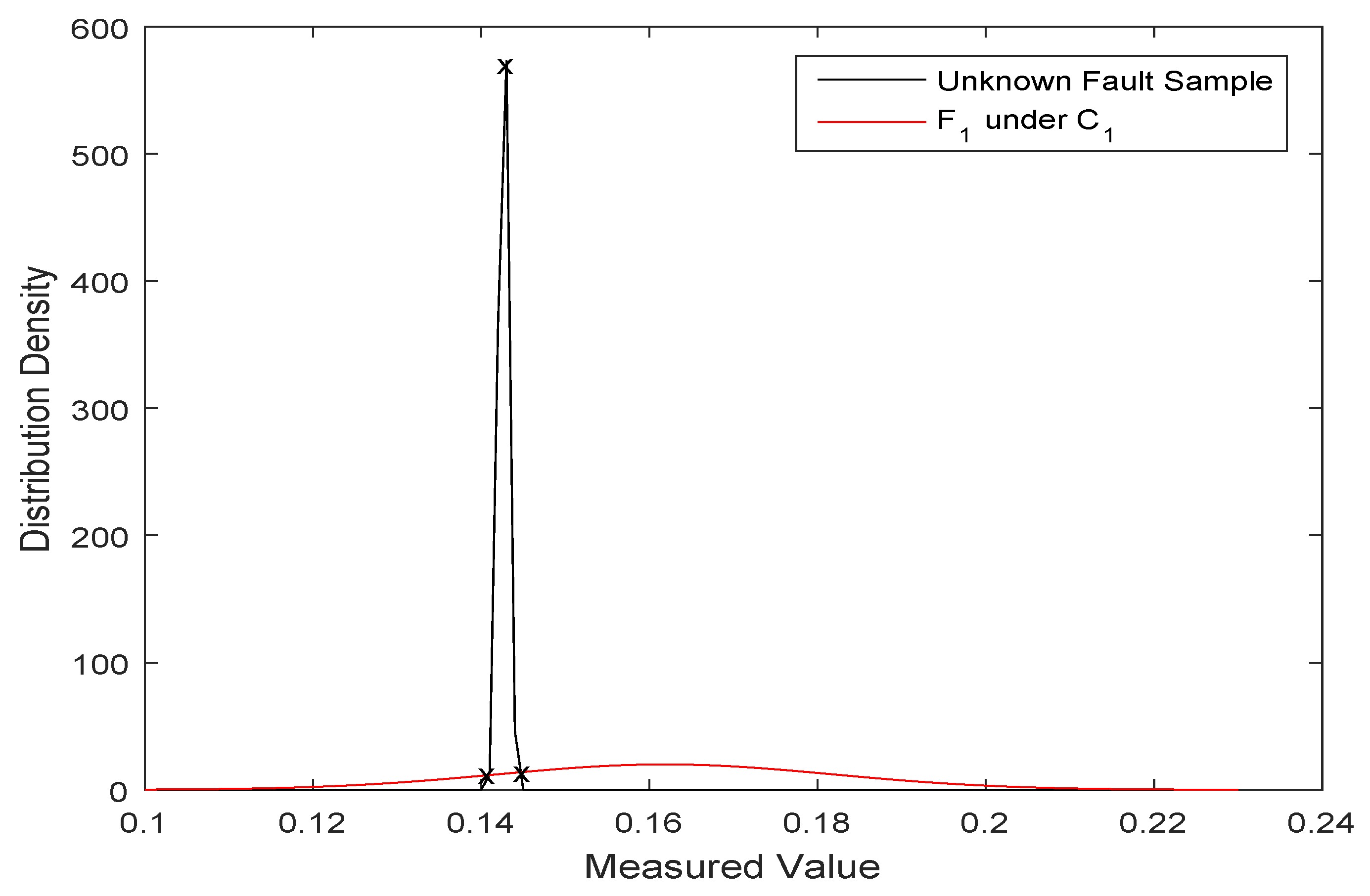
Generate the SNS for the unknown fault sample based on the multi-stage data from each fault type under each feature. Each stage’s data collected is used to establish the normal distribution model. The generated normal distributions of fault types and the unknown fault sample are listed in

Table 2. Multiple distributions of fault types and the unknown fault sample.

Fault Type	Stage	Feature
		${\mathit{C}}_1$	${\mathit{C}}_2$	${\mathit{C}}_3$	${\mathit{C}}_4$
$F_1$	1	$N(0.1619,0.0200)$	$N(0.1538,0.0112)$	$N(0.1163,0.0098)$	$N(4.3057,0.1124)$
	2	$N(0.1596,0.0073)$	$N(0.1509,0.0052)$	$N(0.1095,0.0021)$	$N(4.4143,0.0226)$
	3	$N(0.1644,0.0009)$	$N(0.1468,0.0024)$	$N(0.1063,0.0037)$	$N(4.2626,0.6336)$
	4	$N(0.1617,0.0006)$	$N(0.1519,0.0316)$	$N(0.1117,0.0022)$	$N(4.3138,0.0249)$
	5	$N(0.1598,0.0010)$	$N(0.1428,0.0025)$	$N(0.1182,0.0017)$	$N(4.3319,0.0347)$
$F_2$	1	$N(0.1696,0.0096)$	$N(0.3266,0.0108)$	$N(0.2772,0.0250)$	$N(4.9825,0.1882)$
	2	$N(0.1742,0.0045)$	$N(0.3278,0.0083)$	$N(0.2726,0.0095)$	$N(4.5844,0.1226)$
	3	$N(0.1932,0.0138)$	$N(0.3384,0.0115)$	$N(0.2217,0.0339)$	$N(4.4358,0.4015)$
	4	$N(0.1916,0.0037)$	$N(0.3350,0.0063)$	$N(0.2131,0.0053)$	$N(5.0105,0.6455)$
	5	$N(0.1804,0.0031)$	$N(0.3187,0.0041)$	$N(0.2255,0.0135)$	$N(4.5631,0.0678)$
$F_3$	1	$N(0.3387,0.0071)$	$N(0.3413,0.0207)$	$N(0.1501,0.0120)$	$N(9.8483,0.0709)$
	2	$N(0.3296,0.0026)$	$N(0.3511,0.0090)$	$N(0.1341,0.0080)$	$N(9.7652,0.0953)$
	3	$N(0.3247,0.0074)$	$N(0.3409,0.0135)$	$N(0.1341,0.0113)$	$N(9.7802,0.0608)$
	4	$N(0.3265,0.0049)$	$N(0.3357,0.0098)$	$N(0.1330,0.0052)$	$N(9.8739,0.1267)$
	5	$N(0.3275,0.0023)$	$N(0.3503,0.0060)$	$N(0.1295,0.0048)$	$N(9.7856,0.1010)$
$S_1$	1	$N(0.1427,0.0006)$	$N(0.1109,0.0316)$	$N(0.1337,0.0022)$	$N(4.0938,0.0249)$

. For instance, the normal distribution of ${S_1}_{C_1}$ data and ${F_1}_{C_1}$ with five stages of data is shown in Figure 4. As the figure shows, each stage’s data collected drift to a certain extent in a certain range. In particular, there were distinct differences between the fault types collected in each stage and the data of unknown fault samples. Therefore, it is significant to collect data in multiple stages and to use its integration with the neutrosophic set to deal with the uncertainty of fault information.

Then, $\mu ,\pi ,\nu$ are calculated with Equations (6) and (7). For instance, the distribution of ${S_1}_{C_1}Data$ was $N(0.1427,0.0006)$, the normal distribution of ${F_1}_{C_1}$’s first stage of data was $N(0.1619,0.0200)$, and the membership degree of SNN generated from the two distributions is shown in Figure 5. As the figure shows, the intersection points of distribution between the unknown fault sample ($S_1$) and ${F_1}_{C_1}$’s first stage data are marked with X, and the peak point of $S_1$’s distribution is marked with X in the same way. Then, from the Equations (6) and (7), the SNN was generated and denoted as $(0.0197,0.0969,0.9803)$. The generated SNSs are listed in

Table 3. The generated SNS for $S_1$ based on the multi-stage data from every fault type under every feature.

Fault Type	Stage	Feature
		${\mathit{C}}_1$	${\mathit{C}}_2$	${\mathit{C}}_3$	${\mathit{C}}_4$
$F_1$	1	(0.0197, 0.0969, 0.9803)	(0.7400, 0.5731, 0.2600)	(0.0973, 0.3191, 0.9027)	(0.0841, 0.2888, 0.9159)
	2	(0.0092, 0.0521, 0.9908)	(0.6576, 0.6426, 0.3424)	(0.0000, 0.0000, 1.0000)	(0.0000, 0.0000, 1.0000)
	3	(0.0000, 0.0000, 1.0000)	(0.6382, 0.6545, 0.3618)	(0.0000, 0.0000, 1.0000)	(0.0388, 0.1641, 0.9612)
	4	(0.0000, 0.0000, 1.0000)	(0.8108, 0.4851, 0.1892)	(0.0000, 0.0000, 1.0000)	(0.0001, 0.0006, 0.9999)
	5	(0.0000, 0.0000, 1.0000)	(0.7177, 0.5951, 0.2823)	(0.0004, 0.0032, 0.9996)	(0.0003, 0.0026, 0.9997)
$F_2$	1	(0.0021, 0.0152, 0.9979)	(0.0000, 0.0000, 1.0000)	(0.0000, 0.0000, 1.0000)	(0.0000, 0.0000, 1.0000)
	2	(0.0000, 0.0000, 1.0000)	(0.0000, 0.0000, 1.0000)	(0.0000, 0.0000, 1.0000)	(0.0010, 0.0082, 0.9990)
	3	(0.0001, 0.0010, 0.9999)	(0.0000, 0.0000, 1.0000)	(0.0038, 0.0249, 0.9962)	(0.0486, 0.1944, 0.9514)
	4	(0.0000, 0.0000, 1.0000)	(0.0000, 0.0000, 1.0000)	(0.0000, 0.0000, 1.0000)	(0.0164, 0.0836, 0.9836)
	5	(0.0000, 0.0000, 1.0000)	(0.0000, 0.0000, 1.0000)	(0.0000, 0.0000, 1.0000)	(0.0000, 0.0000, 1.0000)
$F_3$	1	(0.0000, 0.0000, 1.0000)	(0.0001, 0.0008, 0.9999)	(0.1118, 0.3502, 0.8882)	(0.0000, 0.0000, 1.0000)
	2	(0.0000, 0.0000, 1.0000)	(0.0000, 0.0000, 1.0000)	(0.2525, 0.5650, 0.7475)	(0.0000, 0.0000, 1.0000)
	3	(0.0000, 0.0000, 1.0000)	(0.0000, 0.0000, 1.0000)	(0.1847, 0.4785, 0.8153)	(0.0000, 0.0000, 1.0000)
	4	(0.0000, 0.0000, 1.0000)	(0.0000, 0.0000, 1.0000)	(0.3815, 0.6648, 0.6185)	(0.0000, 0.0000, 1.0000)
	5	(0.0000, 0.0000, 1.0000)	(0.0000, 0.0000, 1.0000)	(0.4364, 0.6850, 0.5636)	(0.0000, 0.0000, 1.0000)

.

Step 3

Aggregate the generated SNSs based on each fault type under each feature. Fuse the five stages of SNNs for each fault type under each feature with the SNWA operator, Equation (5). It is assumed that the weights (w) of the five SNNs are $[0.20,0.20,0.20,0.20,0.20]$. For example, the SNNs based on the fault type $F_1$ under feature $C_1$ could be fused as follows:

$$\begin{array}{c}{\alpha }_{11}=SNWA({\alpha }_{11}^1,{\alpha }_{11}^2,{\alpha }_{11}^3,{\alpha }_{11}^4,{\alpha }_{11}^5)\hfill \\ =SNWA\left(\right(0.0197,0.0969,0.9803),(0.0092,0.0521,0.9908),\hfill \\ (0,0,1),(0,0,1),(0,0,1))\hfill \\ =(0.0058,0.0000,0.9942).\hfill \end{array}$$

The others are shown in

Table 4. The results of fusing the five SNNs of each fault type under each feature.

Fault Type	${\mathit{C}}_1$	${\mathit{C}}_2$	${\mathit{C}}_3$	${\mathit{C}}_4$
$F_1$	(0.0058, 0.0000, 0.9942)	(0.7200, 0.5868, 0.2800)	(0.0203, 0.0000, 0.9797)	(0.0252, 0.0008, 0.9748)
$F_2$	(0.0004, 0.0000, 0.9996)	(0.0000, 0.0000, 1.0000)	(0.0008, 0.0000, 0.9992)	(0.0134, 0.0038, 0.9866)
$F_3$	(0.0000, 0.0000, 1.0000)	(0.0000, 0.0000, 1.0000)	(0.2836, 0.5332, 0.7164)	(0.0000, 0.0000, 1.0000)

.

Step 4

Aggregate the fused SNSs based on all features of each fault type. Fusing the SNNs is based on the four features of each fault type by the SNWA operator, Equation (5). In addition, it is supposed the weights (w) of the four SNNs are $[0.25,0.25,0.25,0.25]$. For example, the SNNs based on fault type $F_1$ could be fused as follows:

$$\begin{array}{c}{\alpha }_1=SNWA({\alpha }_{11},{\alpha }_{12},{\alpha }_{13},{\alpha }_{14})\hfill \\ =SNWA\left(\right(0.0058,0,0.9942),(0.72,0.5868,0.28),(0.0203,0,0.9797),\hfill \\ (0.0252,0.0008,0.9748))\hfill \\ =(0.2633,0.0000,0.7367).\hfill \end{array}$$

The others are shown in

Table 5. The results of fusing the SNNs containing four features based on each fault type.

Fault Type	SNS
$F_1$	(0.2633, 0.0000, 0.7367)
$F_2$	(0.0030, 0.0000, 0.9970)
$F_3$	(0.0952, 0.0000, 0.9048)

.

Step 5

Determine the fault type of the unknown fault sample. Finally, Table 5 can be regarded as an SNN fault diagnosis matrix which can be used to rank the three fault types via the defuzzification method (Equation (10)). The descendant ranks of the crisp numbers of the three fault types are shown in

Table 6. The ranks of the crisp numbers of three fault types.

Fault Type	Crisp Number	Rank
$F_1$	0.263335	1
$F_2$	0.003040	3
$F_3$	0.095221	2

.

The above ranking results show that the fault type diagnosed by the proposed method is $F_1$, which is consistent with the true fault type.

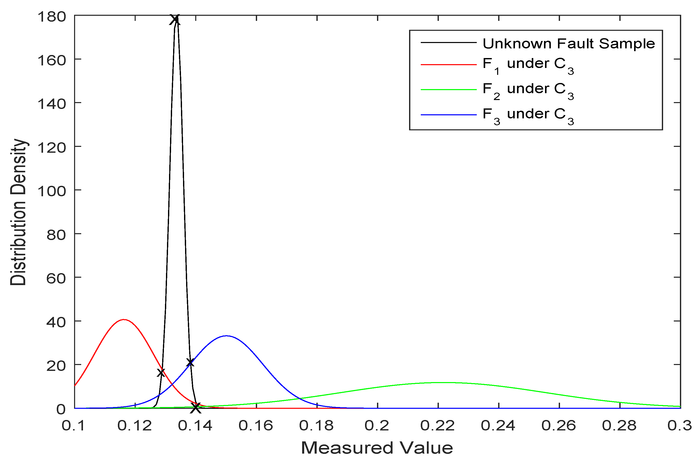
In addition, taking the distribution of the data of $S_1$ under a certain feature, for instance, $C_3$, and the distribution of the first stage’s data of each fault type under the identical feature as an example, the distribution figure is shown in Figure 6. As the figure shows, the maximum intersection points of the ordinate of distribution between $S_1$ and each fault type ($F_i$) are marked with X, and the peak point of $S_1$’s distribution is marked with X in the same way. Then, from the calculation formula of the membership degree (Equation (6)), it is clear that the membership of $S_1$ to $F_3$ is the maximal one, which conflicts with the originally known information that $S_1$’s actual fault type is $F_1$, and this situation is not rare. Therefore, the integration of multi-stage fault template data and the neutrosophic set is efficient and significant, and it fuses the conflicting information into coordinated information and obtains the correct diagnosis results.

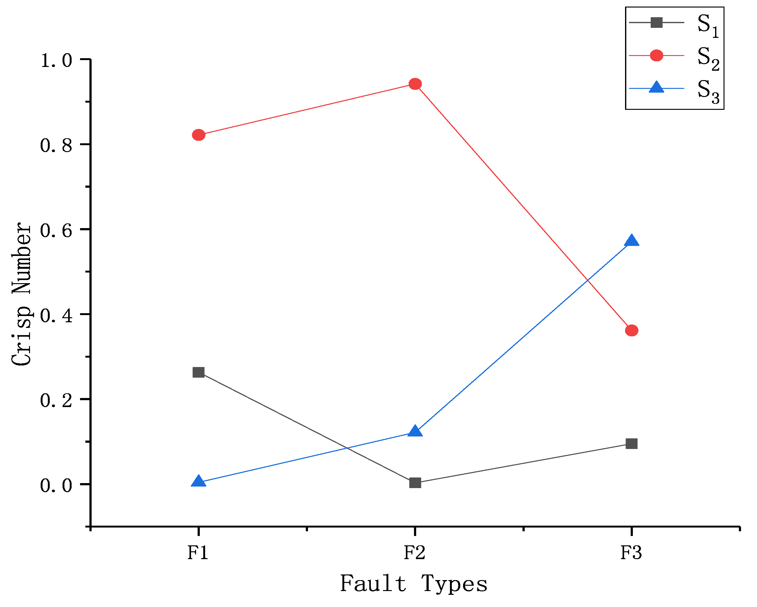
Moreover, the proposed method was used to verify the other two unknown fault samples, and these diagnosis results were also correct. The diagnosis result of the three unknown fault samples are shown in Figure 7, where the ordinate indicates the crisp number of the defuzzification result, and the abscissa indicates the fault types. As shown in this figure, the crisp numbers of the unknown fault sample of each fault type are plotted with a line chart. When the crisp number of an unknown fault sample for a certain fault type ($F_i$) is maximal, the diagnosed fault type of the unknown fault sample is $F_i$.

Compared with Xu’s method [54], which was used to diagnose three unknown fault samples ($S_1,S_2,S_3$), the proposed method was also applied to diagnose identical three unknown fault samples ($S_1,S_2,S_3$) to demonstrate the reasonableness of this proposed method. The diagnosis results are shown in

Table 7. Diagnosis results of the proposed method and Xu’s method.

Unknown Fault	Mehod	Rank of Fault Types			Diagnosis Result	Validity
		F1	F2	F3
$S_1$	The proposed method	1	3	2	$F_1$	$Correct$
	Xu’ method [54]	1	3	2	$F_1$	$Correct$
$S_2$	The proposed method	2	1	3	$F_2$	$Correct$
	Xu’ method [54]	2	1	3	$F_2$	$Correct$
$S_3$	The proposed method	3	2	1	$F_3$	$Correct$
	Xu’ method [54]	3	2	1	$F_3$	$Correct$

.

From the diagnosis results in Table 7, it is concluded that the similar rankings for all fault types and diagnosis results indicates the practicality and effectiveness of the proposed method. Xu’s method [54] only applies to the minimum and maximum mean values of five stages of data, whose boundary rests with the several stages of data collected. However, it is widely admitted that each stage’s data would drift to a certain extent over a certain range, and the deviation of data due to the unsteadiness of the actual environment is one of most influencing causes in fault diagnosis results. It is difficult for Xu’s method [54] to express and deal with the uncertainty of multi-stage fault template data, which the proposed method coped with appropriately due to the integration of multi-stage fault template data and the neutrosophic set. In adition, the crisp numbers fail to precisely express the information extracted from the data collected due to the unsteadiness of measuring the environment. The neutrosophic set, however, was able to accurately describe the uncertain phenomenon, as it gives consideration to both the uncertainty of fault types and the unknown fault sample. Most kinds of uncertain problems in the process of fault diagnosis, including uncertain information and inconsistent information could be handled well with the integration of multi-stage fault template data and the neutrosophic set.

5. Conclusions

In this paper, to deal with uncertain problems in fault diagnosis, a fault diagnosis method was developed by defuzzying the neutrosophic set obtained from multi-stage data. The focus of this method is the collection of data in multiple stages and the generation of SNS, which was expected to appropriately minimize the uncertainty of fault type information and unknown fault sample information. An illustrative example was provided in this paper, and the results of this example indicate that the proposed method can effectively diagnose the fault type of an unknown fault sample. This neutrosophic set based fault diagnosis method based on multi-stage fault template data not only handles the uncertainty of information collected in fault diagnosis well, but also provides a method for fault diagnosis where there are complicated corresponding relationships between multiple fault types and their features. It is both efficient and convenient when dealing with fault diagnosis problems. Further work will focus on the following directions. An appropriate method for the calculation of features’ weights based on the information collected is planned. In addition, for the convenience of calculation, the double aggregation of netrosophic sets may be simplified in future work.

References

- Caliskan, F.; Zhang, Y.; Wu, N.E.; Shin, J.Y. Actuator fault diagnosis in a Boeing 747 model via adaptive modified two-stage Kalman filter. Int. J. Aerosp. Eng. 2014, 2014, 1–10. [Google Scholar] [CrossRef]
- Zieja, M.; Golda, P.; Zokowski, M.; Majewski, P. Vibroacoustic technique for the fault diagnosis in a gear transmission of a military helicopter. J. Vibroeng. 2017, 19, 1039–1049. [Google Scholar] [CrossRef]
- Strydom, J.J.; Miskin, J.J.; McCoy, J.T.; Auret, L.; Dorfling, C. Fault diagnosis and economic performance evaluation for a simulated base metal leaching operation. Miner. Eng. 2018, 123, 128–143. [Google Scholar] [CrossRef]
- Gong, X.; Qiao, W. Bearing fault diagnosis for direct-drive wind turbines via current-demodulated signals. IEEE Trans. Ind. Electron. 2013, 60, 3419–3428. [Google Scholar] [CrossRef]
- Zhang, C.; Li, D.; Broumi, S.; Sangaiah, A.K. Medical diagnosis based on single-valued neutrosophic probabilistic rough multisets over two universes. Symmetry 2018, 10, 213. [Google Scholar] [CrossRef]
- Oliveira, C.C.; Da Silva, J.M. Fault diagnosis in highly dependable medical wearable systems. J. Electron. Test. 2016, 32, 467–479. [Google Scholar] [CrossRef]
- Glowacz, A.; Glowacz, Z. Diagnosis of stator faults of the single-phase induction motor using acoustic signals. Appl. Acoust. 2016, 117, 20–27. [Google Scholar] [CrossRef]
- Gai, J.; Hu, Y. Research on Fault Diagnosis Based on Singular Value Decomposition and Fuzzy Neural Network. Shock Vib. 2018, 2018, 1–7. [Google Scholar] [CrossRef] [Green Version]
- Deng, X.; Xiao, F.; Deng, Y. An improved distance-based total uncertainty measure in belief function theory. Appl. Intell. 2017, 46, 898–915. [Google Scholar] [CrossRef]
- Deng, X.; Jiang, W. Dependence assessment in human reliability analysis using an evidential network approach extended by belief rules and uncertainty measures. Ann. Nucl. Energy 2018, 117, 183–193. [Google Scholar] [CrossRef]
- Deng, X. Analyzing the monotonicity of belief interval based uncertainty measures in belief function theory. Int. J. Intell. Syst. 2018, 33, 1869–1879. [Google Scholar] [CrossRef]
- Xu, S.; Jiang, W.; Deng, X.; Shou, Y. A modified Physarum-inspired model for the user equilibrium traffic assignment problem. Appl. Math. Model. 2018, 55, 340–353. [Google Scholar] [CrossRef]
- Xiao, F. Multi-sensor data fusion based on the belief divergence measure of evidences and the belief entropy. Inf. Fusion 2019, 46, 23–32. [Google Scholar] [CrossRef]
- Tay, F.E.; Shen, L. Fault diagnosis based on rough set theory. Eng. Appl. Artif. Intell. 2003, 16, 39–43. [Google Scholar] [CrossRef]
- Yao, X.; Li, S.; Hu, J. Improving rolling bearing fault diagnosis by DS evidence theory based fusion model. J. Sens. 2017, 2017, 1–14. [Google Scholar] [CrossRef]
- Bian, T.; Zheng, H.; Yin, L.; Deng, Y. Failure mode and effects analysis based on Dnumbers and TOPSIS. Qual. Reliab. Eng. Int. 2018, 34, 501–515. [Google Scholar] [CrossRef]
- Dromigny, A.; Zhu, Y.M. Improving the dynamic range of real-time X-ray imaging systems via Bayesian fusion. J. Nondestruct. Eval. 1997, 16, 147–160. [Google Scholar] [CrossRef]
- Rodrigues, M.A.; Liu, Y.; Bottaci, L.; Rigas, D.I. Learning and diagnosis in manufacturing processes through an executable Bayesian network. In Proceedings of the International Conference on Industrial, Engineering and Other Applications of Applied Intelligent Systems, New Orleans, LA, USA, 19–22 June 2000; pp. 390–396. [Google Scholar]
- Lucas, P.J. Bayesian model-based diagnosis. Int. J. Approx. Reason. 2001, 27, 99–119. [Google Scholar] [CrossRef]
- Basir, O.; Yuan, X. Engine fault diagnosis based on multi-sensor information fusion using Dempster–Shafer evidence theory. Inf. Fusion 2007, 8, 379–386. [Google Scholar] [CrossRef]
- Dempster, A.P. Upper and lower probabilities induced by a multivalued mapping. Ann. Math. Stat. 1967, 38, 325–339. [Google Scholar] [CrossRef]
- Shafer, G. A Mathematical Theory of Evidence; Princeton University Press: Princeton, NJ, USA, 1976. [Google Scholar]
- Jiang, W.; Chang, Y.; Wang, S. A method to identify the incomplete framework of discernment in evidence theory. Math. Probl. Eng. 2017, 2017. [Google Scholar] [CrossRef]
- Jiang, W.; Hu, W. An improved soft likelihood function for Dempster-Shafer belief structures. Int. J. Intell. Syst. 2018, 33, 1264–1282. [Google Scholar] [CrossRef]
- Kaftandjian, V.; Dupuis, O.; Babot, D.; Zhu, Y. Uncertainty modelling using Dempster–Shafer theory for improving detection of weld defects. Pattern Recognit. Lett. 2003, 24, 547–564. [Google Scholar] [CrossRef]
- Glowacz, A. Acoustic based fault diagnosis of three-phase induction motor. Appl. Acoust. 2018, 137, 82–89. [Google Scholar] [CrossRef]
- Glowacz, A.; Glowacz, W.; Glowacz, Z.; Kozik, J. Early fault diagnosis of bearing and stator faults of the single-phase induction motor using acoustic signals. Measurement 2018, 113, 1–9. [Google Scholar] [CrossRef]
- Jozwik, J.; Wac-Wlodarczyk, A.; Michalowska, J.; Kloczko, M. Monitoring of the noise emitted by machine tools in industrial conditions. J. Ecol. Eng. 2018, 19, 83–93. [Google Scholar] [CrossRef]
- Lee, L.; Cheng, Y.; Xie, L.; Jiang, L.; Ma, N.; Lu, M. An integrated method of set pair analysis and association rule for fault diagnosis of power transformers. IEEE Trans. Dielectr. Electr. Insul. 2015, 22, 2368–2378. [Google Scholar]
- He, S.; Xiao, L.; Wang, Y.; Liu, X.; Yang, C.; Lu, J.; Gui, W.; Sun, Y. A novel fault diagnosis method based on optimal relevance vector machine. Neurocomputing 2017, 267, 651–663. [Google Scholar] [CrossRef]
- Xi, W.; Li, Z.; Tian, Z.; Duan, Z. A feature extraction and visualization method for fault detection of marine diesel engines. Meas. J. Int. Meas. Confed. 2017, 116, 429–437. [Google Scholar] [CrossRef]
- Krolczyk, G.M.; Krolczyk, J.B.; Legutko, S.; Hunjet, A. Effect of the disc processing technology on the vibration level of the chipper during operations. Teh. Vjesn. 2014, 21, 447–450. [Google Scholar]
- Merizalde, Y.; Hernandez-Callejo, L.; Duque-Perez, O. State of the art and trends in the monitoring, detection and diagnosis of failures in electric induction motors. Energies 2017, 10, 1056. [Google Scholar] [CrossRef]
- Smarandache, F. A unifying field in logics: Neutrosophic logic. Mult. Valued Logic 1999, 8, 489–503. [Google Scholar]
- Ali, M.; Smarandache, F. Complex neutrosophic set. Neural Comput. Appl. 2017, 28, 1817–1834. [Google Scholar] [CrossRef]
- Zhang, X.; Bo, C.; Smarandache, F.; Park, C. New operations of totally dependent-neutrosophic sets and totally dependent-neutrosophic soft sets. Symmetry 2018, 10, 187. [Google Scholar] [CrossRef]
- Ali, M.; Smarandache, F.; Khan, M. Study on the development of neutrosophic triplet ting and neutrosophic triplet field. Mathematics 2017, 6, 46. [Google Scholar] [CrossRef]
- Li, X.; Zhang, X.; Park, C. Generalized interval neutrosophic choquet aggregation operators and their applications. Symmetry 2018, 10, 85. [Google Scholar] [CrossRef]
- Zadeh, L.A. Fuzzy sets. Inf. Control 1965, 8, 338–353. [Google Scholar] [CrossRef] [Green Version]
- Atanassov, K.T. Intuitionistic fuzzy sets. Fuzzy Sets Syst. 1986, 20, 87–96. [Google Scholar] [CrossRef]
- Jiang, W.; Wei, B.; Liu, X.; Li, X.; Zheng, H. Intuitionistic fuzzy power aggregation operator based on entropy and its application in decision making. Int. J. Intell. Syst. 2018, 33, 49–67. [Google Scholar] [CrossRef]
- Turksen, I.B. Interval valued fuzzy sets based on normal forms. Fuzzy Sets Syst. 1986, 20, 191–210. [Google Scholar] [CrossRef]
- Wang, H.; Smarandache, F.; Zhang, Y.; Sunderraman, R. Single valued neutrosophic sets. In Proceedings of the 8th Joint Conference on Information Sciences, Salt Lake, UT, USA, 21–26 July 2005; pp. 94–97. [Google Scholar]
- Ye, J. A multicriteria decision-making method using aggregation operators for simplified neutrosophic sets. J. Intell. Fuzzy Syst. 2014, 26, 2459–2466. [Google Scholar]
- Liu, P.; Wang, Y. Multiple attribute decision-making method based on single-valued neutrosophic normalized weighted Bonferroni mean. Neural Comput. Appl. 2014, 25, 2001–2010. [Google Scholar] [CrossRef]
- Peng, J.; Wang, J.; Wang, J.; Zhang, H.; Chen, X. Simplified neutrosophic sets and their applications in multi-criteria group decision-making problems. Int. J. Syst. Sci. 2016, 47, 2342–2358. [Google Scholar] [CrossRef]
- Ye, J. Single-valued neutrosophic similarity measures based on cotangent function and their application in the fault diagnosis of steam turbine. Soft Comput. 2017, 21, 817–825. [Google Scholar] [CrossRef]
- Ye, J. Fault diagnoses of hydraulic turbine using the dimension root similarity measure of single-valued neutrosophic sets. Intell. Autom. Soft Comput. 2016, 1–8. [Google Scholar] [CrossRef]
- Kong, L.; Wu, Y.; Ye, J. Misfire fault diagnosis method of gasoline engines using the cosine similarity measure of neutrosophic numbers. Neutrosophic Sets Syst. 2015, 8, 42–45. [Google Scholar]
- Zhang, C.; Zhai, Y.; Li, D.; Mu, Y. Steam turbine fault diagnosis based on single-valued neutrosophic multigranulation rough sets over two universes. J. Intell. Fuzzy Syst. 2016, 31, 2829–2837. [Google Scholar] [CrossRef]
- Jiang, W.; Xie, C.; Zhuang, M.; Tang, Y. Failure Mode and Effects Analysis based on a novel fuzzy evidential method. Appl. Soft Comput. 2017, 57, 672–683. [Google Scholar] [CrossRef]
- He, Z.; Jiang, W. An evidential dynamical model to predict the interference effect of categorization on decision making. Knowl. Based Syst. 2018, 150, 139–149. [Google Scholar] [CrossRef]
- Zheng, X.; Deng, Y. Dependence Assessment in Human Reliability Analysis Based on Evidence Credibility Decay Model and IOWA Operator. Ann. Nucl. Energy 2018, 112, 673–684. [Google Scholar] [CrossRef]
- Xu, X.; Zhou, Z.; Wen, C. Data fusion algorithm of fault diagnosis considering sensor measurement uncertainty. Int. J. Smart Sens. Intell. Syst 2013, 6, 171–190. [Google Scholar]
- Shannon, C.E. A mathematical theory of communication. ACM SIGMOBILE Mob. Comput. Commun. Rev. 2001, 5, 3–55. [Google Scholar] [CrossRef]
- Boran, F.E.; Genç, S.; Kurt, M.; Akay, D. A multi-criteria intuitionistic fuzzy group decision making for supplier selection with TOPSIS method. Expert Syst. Appl. 2009, 36, 11363–11368. [Google Scholar] [CrossRef]
- Xu, X.; Wen, C. Theory and Application of Multi-Source and Uncertain Information Fusion; Science Press: Beijing, China, 2012; pp. 98–108. [Google Scholar]
Figure 1.
Block diagram of the proposed method.
Figure 2.
Distribution of S under and under .
Figure 3.
Generation of the membership degree.
Figure 4.
Distribution of under and under .
Figure 5.
Generation of membership degree.
Figure 6.
The distribution of and the three fault types.
Figure 7.
The diagnosis results of the three unknown fault samples.