Any Pair of 2D Curves Is Consistent with a 3D Symmetric Interpretation

Abstract

Symmetry has been shown to be a very effective a priori constraint in solving a 3D shape recovery problem. Symmetry is useful in 3D recovery because it is a form of redundancy. There are, however, some fundamental limits to the effectiveness of symmetry. Specifically, given two arbitrary curves in a single 2D image, one can always find a 3D mirror-symmetric interpretation of these curves under quite general assumptions. The symmetric interpretation is unique under a perspective projection and there is a one parameter family of symmetric interpretations under an orthographic projection. We formally state and prove this observation for the case of one-to-one and many-to-many point correspondences. We conclude by discussing the role of degenerate views, higher-order features in determining the point correspondences, as well as the role of the planarity constraint. When the correspondence of features is known and/or curves can be assumed to be planar, 3D symmetry becomes non-accidental in the sense that a 2D image of a 3D asymmetric shape obtained from a random viewing direction will not allow for 3D symmetric interpretations.

1. Introduction

Curves in a 2D image provide very effective information about the 3D shape “out there” [1]. Figure 1 shows a simple example. The reader can easily see the 3D shape of the closed contour even though the image itself is 2D. Demo 1 [2] illustrates the 3D interpretation that agrees with what the reader perceives by looking at Figure 1. The 3D recovery shown in the Demo used 3D symmetry as a constraint. This informal observation is consistent with results of a number of psychophysical experiments. Specifically, it has been shown that humans can perceive 3D shapes of objects and recognize the objects as effectively from line drawings as from realistic images [1,3,4,5]. Furthermore, the 3D percept is usually close to veridical. We have recently presented a computational model that can recover 3D shape of a symmetric or approximately symmetric 3D object from a single 2D image (line drawing) of this object. The model does this by applying a priori constraints to a 3D interpretation of an image of the object’s contours. The a priori constraints included: mirror-symmetry of the 3D shape, planarity of its contours, maximum 3D compactness and minimum surface area of the convex hull of the 3D contours [6,7,8,9,10,11].

A 3D symmetry is a natural prior in recovering 3D shapes from 2D images. Most objects in our natural environment are at least approximately symmetric: animal and human bodies [12], as well as many man-made objects are mirror symmetric, trees and flowers are rotationally symmetric and limbs and torsos of animals are characterized by translational symmetry. Clearly, if a vision system of a human or a robot can assume that the object in front of her is symmetric, the 3D shape recovery becomes much easier. How much easier? Consider mirror-symmetry. Vetter and Poggio [13] showed that a single 2D orthographic image of a mirror-symmetric 3D shape determines this shape with only one unknown parameter. If a 2D perspective image is used, the 3D shape recovery is unique [14,15,16,17]. In these models, the contour-configural organization was provided to the model by a human user. By “contour-configural organization” we mean: finding contours in the image, determining which contours and features in the image correspond to symmetric contours and features in the 3D interpretation, which contours are co-planar and which contours are on the symmetry plane. Note that what we call “contour-configural organization” is similar to the traditional phenomenon called perceptual organization. The main difference is that contour-configural organization incorporates operations such as establishing symmetry and coplanarity in the 3D interpretation. These operations go beyond the traditional perceptual organization. We decided to introduce this new concept (following the suggestion of the Editor) because we want to emphasize that the processes we include are related to the emergence of the percept of the shape of an object, not to arbitrary grouping of features in the image. Establishing contour-configural organization is natural and easy to a human observer. However, we are still far from understanding the underlying mechanisms and there is no computer vision algorithm whose performance in establishing contour-configural organization comes even close to that of a human observer.

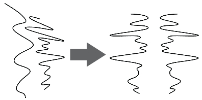
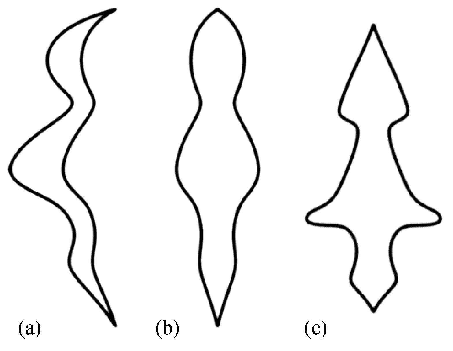
Can a symmetry constraint be applied to an image for which contour-configural organization has not been established? In other words, can 3D symmetry, itself, be used as a tool in establishing contour-configural organization? The answer is, in a general case, negative. Under quite general assumptions, any pair of 2D curves is consistent with 3D symmetric interpretations. For example, a pair of 2D curves in Figure 2a does not look like a 2D projection of a symmetric pair of 3D curves. However, they can be actually interpreted as a symmetric pair of 3D curves by allowing the degenerate (accidental) view of the 3D curves (Figure 2b). Namely, some characteristic features of the 3D symmetric curves become hidden in the depth direction (see Discussion). The reader can see pairs of 2D curves (Figure 1, Figure 2, Figure 3, Figure 5, Figure 7, Figure 8, Figure 12 and Figure 13) and their 3D symmetric interpretations in our online demos [2]. Note that this paper focuses on the process of “constructing” or “interpreting”, rather than “recovering” or “re-constructing” a 3D shape from a 2D line drawing. When a 3D shape is being re-constructed from a line drawing, it is assumed that this line drawing is a 2D projection produced by some 3D object. For the reconstruction to be accurate, it is necessary to know whether the 2D image is a result of a perspective or an orthographic projection and whether the 3D object was symmetric, in the first place. Depending on the actual projection type, the reconstruction may or may not be unique. In this paper, we do not have to know what the actual projection type is and whether the 3D object was symmetric. In fact, the 3D object did not have to exist; the 2D image could have been drawn by an artist without any reference to a 3D object. So, we can assume here the type of projection and then we can always construct a 3D symmetric shape. This is why we use the word “3D interpretation”, rather than “3D reconstruction” throughout this paper. As a consequence of constructing, rather than reconstructing, we are not concerned whether the 3D interpretation is accurate or not. In particular, even if the 2D image was produced by an asymmetric 3D shape, 3D symmetric interpretations exist. The concept of accuracy is irrelevant here.

In Section 2, it is formally stated and proved that any pair of sufficiently “regular” 2D curves can be interpreted as a symmetric pair of 3D curves. This is proved by showing how a symmetric pair of 3D curves is produced from the pair of 2D curves. The main idea behind the proofs is fairly simple. Take a pair of points p_i and q_i in the 2D image. There is always a pair of 3D points P_i and Q_i, whose images are p_i and q_i, such that P_i and Q_i are symmetric with respect to some plane. The symmetry plane bisects the line segment P_iQ_i and is orthogonal to this segment. There are infinitely many such solutions. The individual theorems specify the family of these solutions for perspective and orthographic projections and show that if the image curves are continuous, the 3D symmetric interpretations are also continuous, for both one-to-one and many-to-many point correspondences. First, we provide a proof for a simple case where there is a unique correspondence of pairs of symmetric points. We then generalize the theorems to the case of multiple correspondences. In Section 3, we discuss the role of symmetry in contour-configural organization, as well as the role of other constraints in detecting symmetry from a single 2D image.

2. Theorems and Proofs

We begin with notation. Consider two curves Φ and Ψ in a 3D space and their 2D images φ and ψ. Let Φ and Ψ be symmetric with respect to a plane Π_s, whose normal is n_s(n_x, n_y, n_z). Let P_i(x_Φi, y_Φi, z_Φi), be a point on Φ and Q_i(x_Ψi, y_Ψi, z_Ψi) be its symmetric counterpart on Ψ. Symmetry line segments, which are line segments connecting pairs of corresponding points on Φ and Ψ are parallel to the normal of Π_s in the 3D space. Perspective images of these lines intersect at the vanishing point v on the image plane. The 3D orientation of Π_s is specified by its slant σ_s and tilt τ_s. Without restricting generality, assume τ_s = 0. Note that when τ_s is not zero, we can always rotate the 3D coordinate system around the z-axis by τ_s. Under this assumption, the normal to the symmetry plane is n_s(n_x, 0, n_z). The slant of the symmetry plane is σ_s = atan(n_x/n_z).

In the following theorems, let z = 0 be the image plane Π_I and the x- and y-axes of the 3D Cartesian coordinate system be the 2D coordinate system on the image plane. Let the center of projection F be on the positive side of the z-axis of the 3D Cartesian coordinate system: z_f > 0 where z_f is a z-value of F.

We assume in this paper that 2D curves in Π_s are finitely long and tame:

Definition 1:

A 2D curve is tame when it is connected and composed of a finite number of C² arcs that have following properties; each arc is twice continuously differentiable and a tangent line at every non-endpoint of the arc does not have any intersection with the arc.

Tame curves have finite number of inflections and turns. The definition excludes, for example, pathological curves (like fractal curves), which have infinitely many inflections or turns (see [18] for further discussion).

2.1. A Pair of 2D Curves with Unique Correspondences—The Case of a Perspective Projection

We first consider the case of a perspective projection. The equivalent theorem for an orthographic projection will be proved as a special case of a perspective projection. Theorem 1 states that for any pair of curves in the 2D image, there exists a pair of 3D curves that are symmetric with respect to a plane. The gist of the proof is as follows. Given a pair of 2D curves, the vanishing point of a perspective projection is computed from the endpoints of the curves. The vanishing point determines unique point correspondences between the two curves. It also determines the symmetry plane uniquely for a given position of the center of perspective projection F. Given the plane of symmetry, for any pair of 2D points it is always possible to find a pair of 3D points that are mirror symmetric with respect to this plane.

Theorem 1:

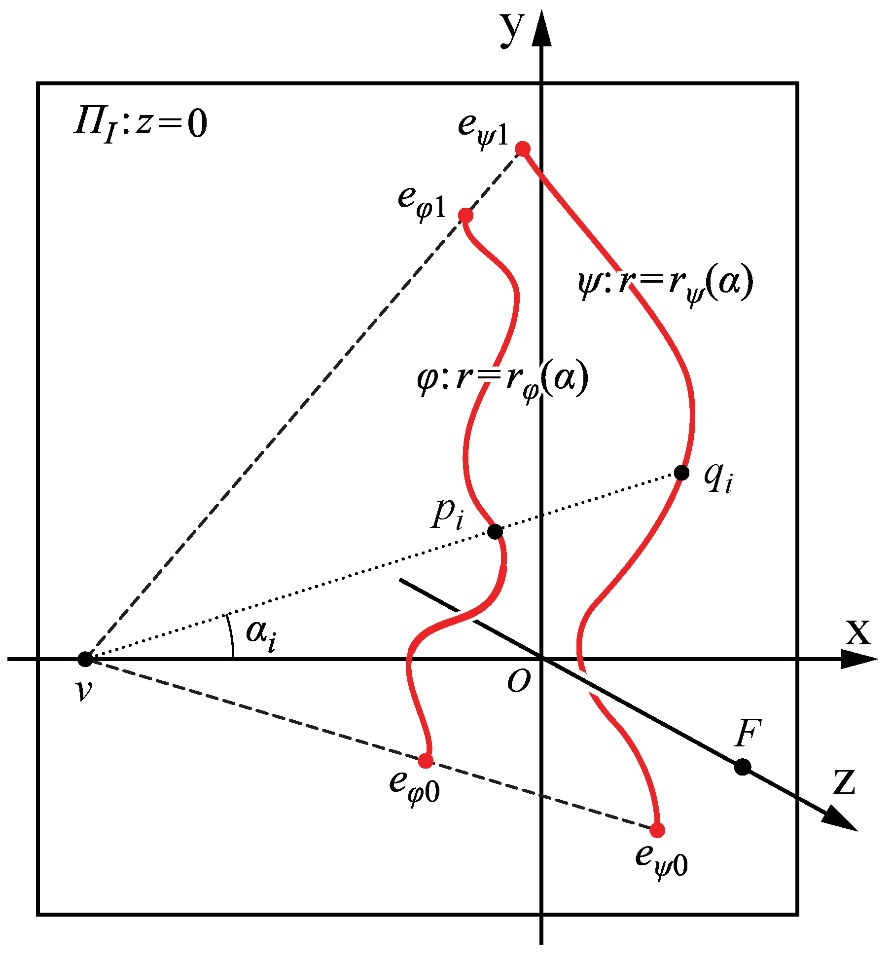
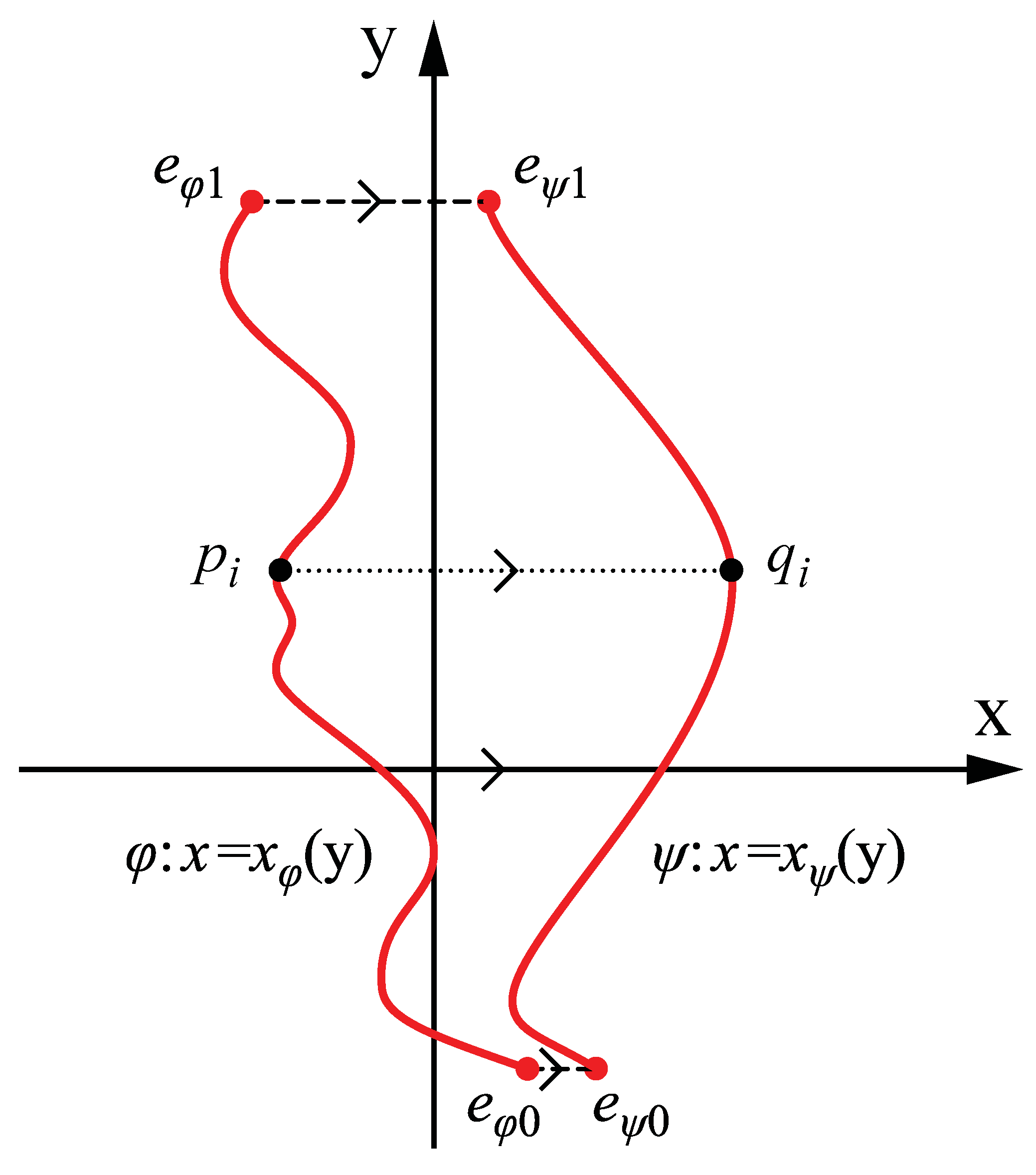
Let φ and ψ be curves in a 2D image that are tame. Let the endpoints of φ be e_φ0 and e_φ1, and the endpoints of ψ be e_ψ0 and e_ψ1. Assume that the lines e_φ0e_ψ0 and e_φ1e_ψ1 intersect at a point v that (i) is not on φ or ψ and (ii) is not between e_φ0 and e_ψ0 or between e_φ1 and e_ψ1. Additionally, assume that each half line that emanates from v and intersects φ has a unique intersection with ψ and vice versa (see Figure 3). Then, for a given center of projection F there exists a pair of continuous curves Φ and Ψ and a plane Π_s in a 3D space such that Φ and Ψ are mirror-symmetric with respect to Π_s and that φ is a perspective projection of Φ and ψ is a perspective projection of Ψ.

Proof:

Figure 3. F = [0, 0, z_f] is the center of perspective projection and Π_I (z = 0) is the image plane. φ and ψ are two given curves on the image plane. e_φ0 and e_φ1 are the endpoints of φ, and e_ψ0 and e_ψ1 are the end points of ψ. The lines e_φ0e_ψ0 and e_φ1e_ψ1 intersect at point v on the x-axis. A line that is emanating from v and intersects with φ has a unique intersection with ψ and vice versa.

Figure 3. F = [0, 0, z_f] is the center of perspective projection and Π_I (z = 0) is the image plane. φ and ψ are two given curves on the image plane. e_φ0 and e_φ1 are the endpoints of φ, and e_ψ0 and e_ψ1 are the end points of ψ. The lines e_φ0e_ψ0 and e_φ1e_ψ1 intersect at point v on the x-axis. A line that is emanating from v and intersects with φ has a unique intersection with ψ and vice versa.

In order to prove this theorem, we have to show that for any pair of corresponding points on φ and ψ, we can find their backprojections in the 3D space, such that these backprojected points are mirror-symmetric with respect to the same plane Π_s. That is, the line segment connecting the backprojected points is bisected by Π_s and parallel to the normal of Π_s. It will be also shown that the backprojected points form a pair of continuous curves.

Let’s set the direction of x-axis so that the vanishing point v is on the x-axis, v = [x_v, 0, 0]. We express φ and ψ in a polar coordinate system (r, α), where r is the distance from the vanishing point v and α is the angle measured relative to the direction of the x-axis. Then, the point p_i = [x_φi, y_φi, 0] = [x_v + r_φ(α_i)cosα_i, r_φ(α_i)sinα_i, 0] on φ and the point q_i = [x_ψi, y_ψi, 0] = [x_v + r_ψ(α_i)cosα_i, r_ψ(α_i)sinα_i, 0] on ψ are corresponding. Note that both r_φ(α) and r_ψ(α) are continuous functions and they are always positive (r_φ(α), r_ψ(α) > 0). Let the equation of the symmetry plane Π_s be: P_i and Q_i, the 3D inverse perspective projections of p_i and q_i, are symmetric with respect to Π_s if and only if they satisfy the following two requirements: the line segment connecting P_i and Q_i is parallel to the normal of Π_s and is bisected by Π_s.

The following equation represents the fact that the line segment connecting P_i and Q_i is parallel to the normal of the plane Π_s: Note that in an inverse perspective projection, an image point [x, y, 0] projects to a 3D point [x(z_f – z)/z_f, y(z_f – z)/z_f, z]. Hence, P_i = [(z_f – z_Φi)(x_v + r_φ(α_i)cosα_i)/z_f, (z_f – z_Φi)r_φ(α_i)sinα_i/z_f, z_Φi] and Q_i = [(z_f – z_Ψi)(x_v + r_ψ(α_i)cosα_i)/z_f, (z_f – z_Ψi)r_ψ(α_i)sinα_i/z_f, z_Ψi]. Then, combining (1) and (2), we obtain: From Equation (3), we obtain the following three facts. First, –d/c is an intersection of the symmetry plane Π_s and the z-axis; it specifies the position of Π_s. Second, the normal to this plane is [– x_v/z_f, 0, 1], which is parallel to a vector [x_v, 0, – z_f] connecting the center of perspective projection with the vanishing point. This immediately follows from the fact that v is the vanishing point corresponding to the lines connecting the pairs of 3D symmetric points, which are all normal to the symmetry plane. Third, a vanishing line (horizon) h of Π_s is parallel to the y-axis on the image plane Π_I. The line h intersects x-axis at: The next equation represents the fact that the line segments connecting pairs of 3D symmetric points are bisected by the symmetry plane. Let M_i be the midpoint between P_i and Q_i –the midpoint lies on the symmetry plane Π_s: From Equations (2) and (5), a perspective projection of M_i to the image plane Π_I can be written as follows: Equation (6) shows that m_i is on a 2D line segment p_iq_i and is determined only by 2D image features on Π_I. It does not depend on the position of the center of projection F. Recall that both r_φ(α) and r_ψ(α) are continuous functions and they are always positive (r_φ(α), r_ψ(α) > 0). It follows that the midpoints of the corresponding pairs of points on φ and ψ form a 2D continuous curve between φ and ψ on Π_I. From Equations 2–6, we have: It is obvious that (7) and (8) represent continuous functions unless m_i is on h: x_mi = x_h. Using Equations (6) and (4), we can rewrite x_mi = x_h as follows: Note that the left-hand side of Equation (9) is a cross-ratio [x_v + r_φ(α_i)cosα_i, x_v + r_ψ(α_i)cosα_i; x_v, x_h] = [x_φi, x_ψi; x_v, x_h]. If x_mi = x_h, z_Φi and z_Ψi diverge to ±∞ and Φ and Ψ are not continuous. This is because a projecting line emanating from F and going through m_i does not intersect Π_s. As a result, M_i, which should be a midpoint between P_i and Q_i, cannot be determined. Recall that 2D projections of midpoints of 3D symmetric pairs of points form a 2D continuous curve on Π_I. Hence, this curve must not have any intersection or tangent point with h. The whole curve must be either to the left or right of h. It follows that the denominators in (7) and (8) must be always positive or always negative for given φ and ψ. If this criterion is not satisfied, the 3D curves will not be continuous. Note that if the position of the center of projection F is a free parameter (this happens when the camera is uncalibrated), it is always possible to set F and thus h so that the criterion for continuity will be satisfied because the curve connecting the midpoints does not depend on F.

Note that d/c is the only free parameter in Equations (7) and (8), once the vanishing point and the center of projection are fixed. Specifically, Equations (7) and (8) show that the left-hand sides are linear functions of d/c. Recall that in an inverse perspective projection, an image point [x, y, 0] projects to a 3D point [x(z_f – z)/z_f, y(z_f – z)/z_f, z]. Assume that d/c ≠ – z_f —otherwise, the 3D interpretation will be degenerate with all the 3D points coinciding with the center of perspective projection F (Except for the case when the symmetry plane coincides with the YOZ plane. This can happen when the image curves are themselves symmetric). It can be seen that d/c determines the size, but not the shape of the 3D curves Φ and Ψ; z_f + d/c is a scale factor with respect to F as a center of scaling. Recall that the denominators in (7) and (8) must be always positive or always negative. From Equations (7) and (8), d/c can be adjusted so that Φ and Ψ are in front of the center of projection F and the image plane Π_I. The symmetric pair of 3D curves produced from the curves in Figure 3 using Equations (7) and (8) is shown in Figure 4.

In this proof, it was assumed that the position of the vanishing point v is known or can be computed from the given 2D image. If the position of the vanishing point on the image plane is not known or is uncertain in the 2D image, the shape of the 3D symmetric interpretation is defined up to two free parameters [19]. These two unknown parameters correspond to the slant and tilt of the symmetry plane Π_s.

2.2. A Pair of 2D Curves with Unique Symmetric Correspondences—the Case of an Orthographic Projection

An orthographic projection is produced from a perspective projection by moving the center of perspective projection to infinity. As a result, the vanishing point corresponding to the symmetry line segments is also moved to infinity regardless of the slant of the symmetry plane. This implies that the 3D symmetric interpretation is always possible regardless of the position of the 2D curves on the image plane. In other words, the criteria for deciding whether the 3D curves are behind or in front of the camera are irrelevant in the case of an orthographic projection. We begin with modifying Equations (7) and (8) so that the position of the vanishing point is expressed as a function of the focal length of the camera. It will then be easy to transform the equations representing a perspective projection to equations representing an orthographic projection.

Under a perspective projection, the projected symmetry line segments in Π_I intersect at a vanishing point v. Since v is an intersection of Π_I and a line which emanates from F and is parallel to n_s, the position of v is [x_v, 0, 0] = [–z_f tanσ_s, 0, 0]. The sine and cosine of the slant σ_s of the symmetry plane Π_s can be expressed as follows: where L is the distance between the vanishing point v and the center of projection F: Let P_i = [x_Φi, y_Φi, z_Φi], be a point on Φ and Q_i = [x_Ψi, y_Ψi, z_Ψi] be its symmetric counterpart on Ψ. Recall that the symmetry line segments are parallel to the normal n_s of the symmetry plane Π_s and n_s = [sinσ_s, 0, cosσ_s]. Hence, y_Φi = y_Ψi. Let, p_i = [x_φi, y_φi, 0] be a perspective image of P_i and q_i = [x_ψi, y_ψi, 0] be a perspective image of Q_i in Π_I. A line segment connecting P_i and Q_i is a symmetry line segment and a line segment connecting p_i and q_i is a projected symmetry line segment; recall that a projected symmetry line segment intersects the x-axis at v. The p_i and q_i were represented in a polar coordinate system and written as p_i = [x_φi, y_φi, 0] = [x_v + r_φicosα_i, r_φisinα_i, 0] and q_i = [x_ψi, y_ψi, 0] = [x_v + r_ψicosα_i, r_ψisinα_i, 0], where r_φi and r_ψi are the distances of p_i and q_i from v when α = α_i. Note that the 3D points P_i and Q_i and their 2D projections p_i and q_i satisfy Equations (7) and (8). From Equations (7), (10) and (11), we obtain z_Φi (an analogous formula can be written for z_Ψi): Recall that an orthographic projection is produced from a perspective projection by moving the center of projection F to infinity: z_f → +∞. As z_f goes to infinity, L goes to positive infinity, as well. From Equation (12), the limit of z_Φi as z_f goes to infinity is: The limit of z_Ψi is obtained in an analogous way: Recall that in an inverse perspective projection, an image point [x, y,0] projects to a 3D point [x(z_f – z)/z_f, y(z_f – z)/z_f, z]. As z_f goes to infinity, the limit of [x(z_f – z)/z_f, y(z_f – z)/z_f, z] is [x, y, z], which is an inverse orthographic projection of [x, y, 0].

Note that x_v goes to negative infinity as z_f goes to infinity; it follows that all α_i become zero. This means that the projected symmetry line segments become parallel to one another and to the x-axis, and the vanishing point v goes to infinity. Hence, the slant σ_s of the symmetry plane cannot be computed from the 2D image; instead, σ_s becomes a free parameter in the 3D interpretation under an orthographic projection. It follows that there are infinitely many 3D symmetric curves that are consistent with a pair of 2D curves φ and ψ. In other words, the 3D curves form a one-parameter family characterized by σ_s; σ_s changes the aspect ratio and the orientation of the 3D shapes of the curves Φ and Ψ [10]. Note that if sin2σ_s = 0 (σ_s is 0 or 90°), z_Φi and z_Ψi diverge to ±∞. Hence, σ_s should not be 0 or 90°. These two cases correspond to degenerate views of Φ and Ψ. When σ_s is 0°, the symmetry plane is parallel to the image plane; φ and ψ will then coincide with each other in the 2D image. In such a case, the 3D recovery of a pair of symmetric 3D curves becomes trivial: one produces any Φ from ϕ and then Ψ is obtained as a mirror reflection of Φ. When σ_s is 90°, the symmetry plane is perpendicular to the image plane. In such a case, φ and ψ, themselves, must be mirror symmetric in the 2D image in order for the 3D symmetric interpretation to exist. But then, the 2D curves themselves represent one possible 3D symmetric interpretation. The ratio d/c is another free parameter, but it only changes the position of Φ and Ψ along the z-axis and does not change their 3D shapes or orientations. From these results, Theorem 1 for a perspective projection generalizes to Theorem 2 for an orthographic projection.

Theorem 2:

Let φ and ψ be curves that are tame in a single 2D image. Let the endpoints of φ be e_φ0 and e_φ1, and the endpoints of ψ be e_ψ0 and e_ψ1. Assume that φ and ψ have the following properties: (i) e_φ0e_ψ0||e_φ1e_ψ1 and (ii) a line that is parallel to e_φ0e_ψ0 and intersects with φ has a unique intersection with ψ and vice versa (see Figure 5). Then, there exist infinitely many pairs of continuous curves Φ and Ψ and a plane Π_s in a 3D space, such that Φ and Ψ are mirror-symmetric with respect to Π_s and that φ is an orthographic projection of Φ and ψ is an orthographic projection of Ψ.

Proof:

Figure 5. φ and ψ are two 2D curves. e_φ0 and e_φ1 are the endpoints of φ, and e_ψ0 and e_ψ1 are the end points of ψ. The lines e_φ0e_ψ0 and e_φ1e_ψ1 are parallel to the x-axis and do not have any intersection with φ and ψ. A line that is parallel to e_φ0e_ψ0 and intersects with φ has a unique intersection with ψ and vice versa.

Figure 5. φ and ψ are two 2D curves. e_φ0 and e_φ1 are the endpoints of φ, and e_ψ0 and e_ψ1 are the end points of ψ. The lines e_φ0e_ψ0 and e_φ1e_ψ1 are parallel to the x-axis and do not have any intersection with φ and ψ. A line that is parallel to e_φ0e_ψ0 and intersects with φ has a unique intersection with ψ and vice versa.

Let the orientations of the line segments e_φ0e_ψ0 and e_φ1e_ψ1 be horizontal. This does not restrict the generality: if these line segments are not horizontal, we rotate the image so that they become horizontal. For any point p_i = [x_φi, y_φi] on φ, we find its counterpart on ψ as q_i = [x_ψi, y_ψi]. Note that q_i is found as an intersection of ψ and a horizontal line y = y_φi. Hence, y_φi = y_ψi. We assume that this intersection is unique. Then, both φ and ψ can be represented as functions of y: x_φi = x_φ(y_φi) and x_ψi = x_ψ(y_φi). From Equations (13) and (14), the 3D symmetric curves Φ and Ψ are produced by computing the positions of all points P_i and Q_i as follows: where σ_s is a slant of the symmetry plane. The tilt τ_s of the symmetry plane is zero. Equations (15) and (16) allow one to compute a pair of 3D symmetric curves Φ and Ψ from a pair of 2D curves φ and ψ under an orthographic projection. It is obvious from these equations that Φ and Ψ are continuous when φ and ψ are continuous. Recall that slant σ_s is a free parameter; it can be arbitrary, except for sin2σ_s = 0. So, the 3D symmetric curves form a one-parameter family characterized by σ_s. Equations (15–16) show that a relation between the pair of 2D curves φ and ψ and the pair of 3D curves Φ and Ψ becomes computationally simple when σ_s is 45° (or – 45°) and d/c is 0; the absolute value of the z-coordinate of Q_i is equal to the x-coordinate of P_i and the absolute value of the z-coordinate of P_i is equal to the x-coordinate of Q_i. The symmetric pair of 3D curves produced using Equations (15) and (16) and consistent with φ and ψ in Figure 5 is shown in Figure 6.

If the direction of the lines connecting the corresponding points on φ and ψ is not known or is uncertain, the family of 3D interpretations is characterized by two parameters: slant and tilt of the symmetry plane.

2.3. A Pair of 2D Curves with Multiple Symmetric Correspondences

In the two theorems above, it was assumed that correspondences between points of φ and ψ are unique. We generalize these theorems to the case of non-unique correspondences. A point on φ can have multiple corresponding points on ψ (and vice versa). In such a case, the 3D interpretation of φ will have segments whose 2D projections perfectly overlap one another in the 2D image (Figure 7). In other words, the 3D symmetry will be hidden in the depth direction, and thus, the 3D view will be degenerate (see Discussion). First, we consider the case of an orthographic projection. This case will then be generalized to a perspective projection.

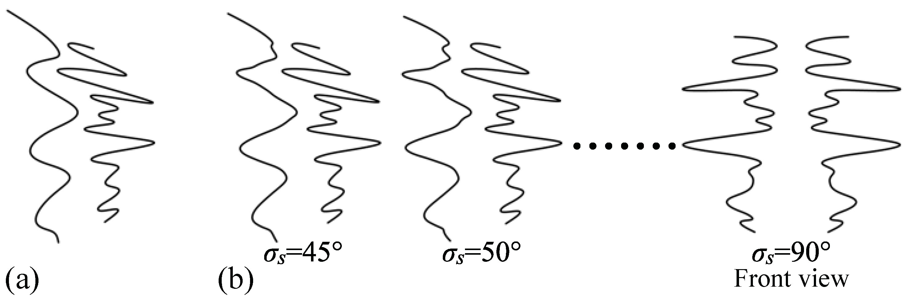
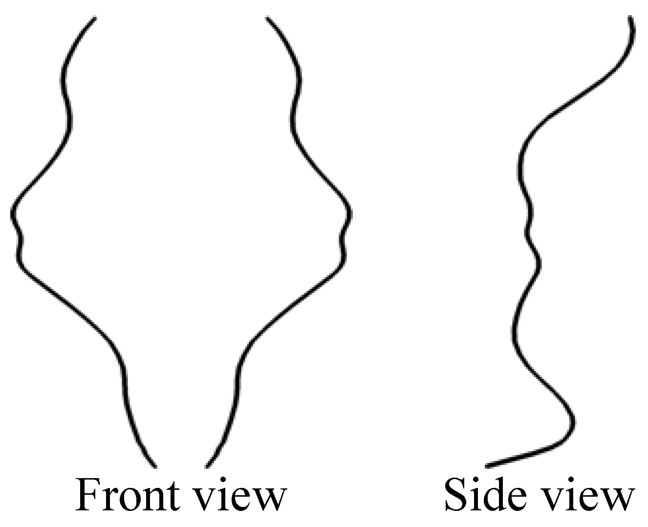
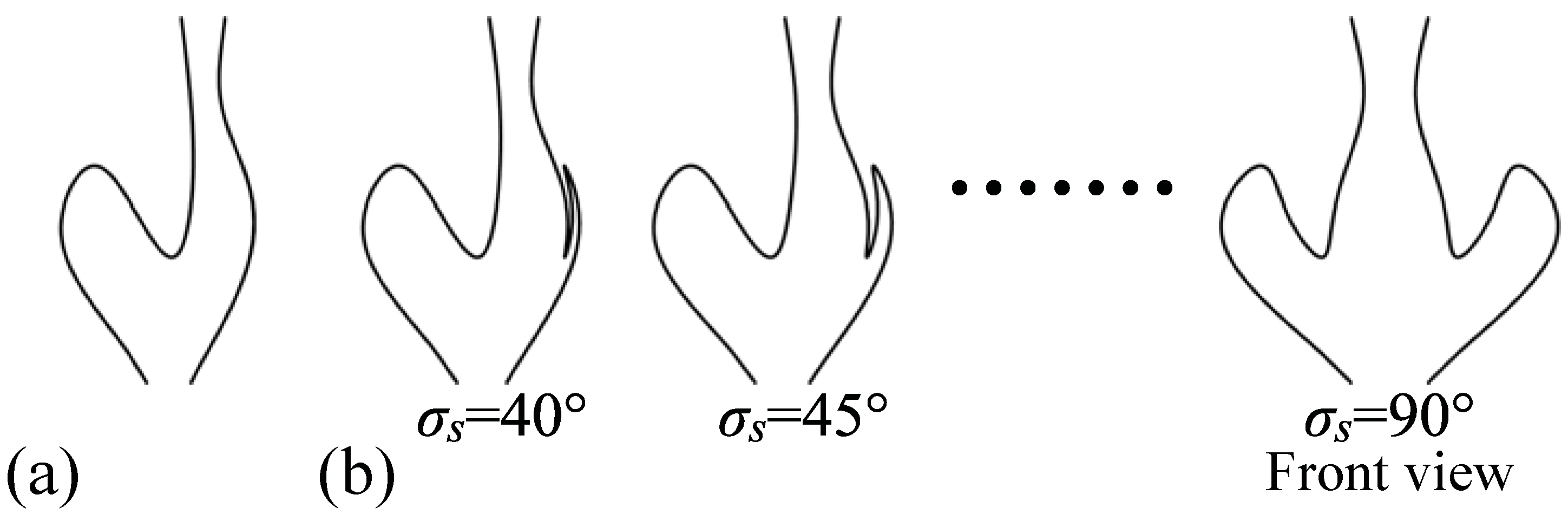
Figure 7. An asymmetric pair of 2D curves with multiple symmetric correspondences and its 3D symmetric interpretation. (a) An asymmetric pair of 2D curves. Some points of the right curve correspond to three points of the left curve. These curves can be still interpreted as a 2D orthographic projection of a symmetric pair of 3D curves. The slant σ_s of the symmetry plane was set to 35°; (b) Three different views of the 3D symmetric interpretation produced from the pair of the 2D curves in (a). The numbers in the bottom are the values of the slant σ_s of the symmetry plane of the symmetric pair of the 3D curves. For σ_s equal to 35°, the image is identical to that in (a). When σ_s is 90°, its 2D projection itself becomes symmetric. See Demo 5 in supplemental material for an interactive illustration of the 3D symmetric curves [2].

Figure 7. An asymmetric pair of 2D curves with multiple symmetric correspondences and its 3D symmetric interpretation. (a) An asymmetric pair of 2D curves. Some points of the right curve correspond to three points of the left curve. These curves can be still interpreted as a 2D orthographic projection of a symmetric pair of 3D curves. The slant σ_s of the symmetry plane was set to 35°; (b) Three different views of the 3D symmetric interpretation produced from the pair of the 2D curves in (a). The numbers in the bottom are the values of the slant σ_s of the symmetry plane of the symmetric pair of the 3D curves. For σ_s equal to 35°, the image is identical to that in (a). When σ_s is 90°, its 2D projection itself becomes symmetric. See Demo 5 in supplemental material for an interactive illustration of the 3D symmetric curves [2].

Theorem 3:

Let φ and ψ be curves that are tame in a 2D image. Let the endpoints of φ be e_φ0 and e_φ1, the endpoints of ψ be e_ψ0 and e_ψ1. Let a line connecting e_φ0 and e_ψ0 be l₀ and that connecting e_φ1 and e_ψ1 be l₁. Assume that φ and ψ have the following properties: (i) l₀||l₁, (ii) l₀ and l₁ do not have any intersection with φ and ψ and (iii) a line that is parallel to l₀ and intersects φ has one or a finite number of intersections with ψ and vice versa (see Figure 8). Then, there exist infinitely many pairs of continuous curves Φ and Ψ and a plane Π_s in a 3D space, such that Φ and Ψ are mirror-symmetric with respect to Π_s and that φ is an orthographic projection of Φ and ψ is an orthographic projection of Ψ.

Proof:

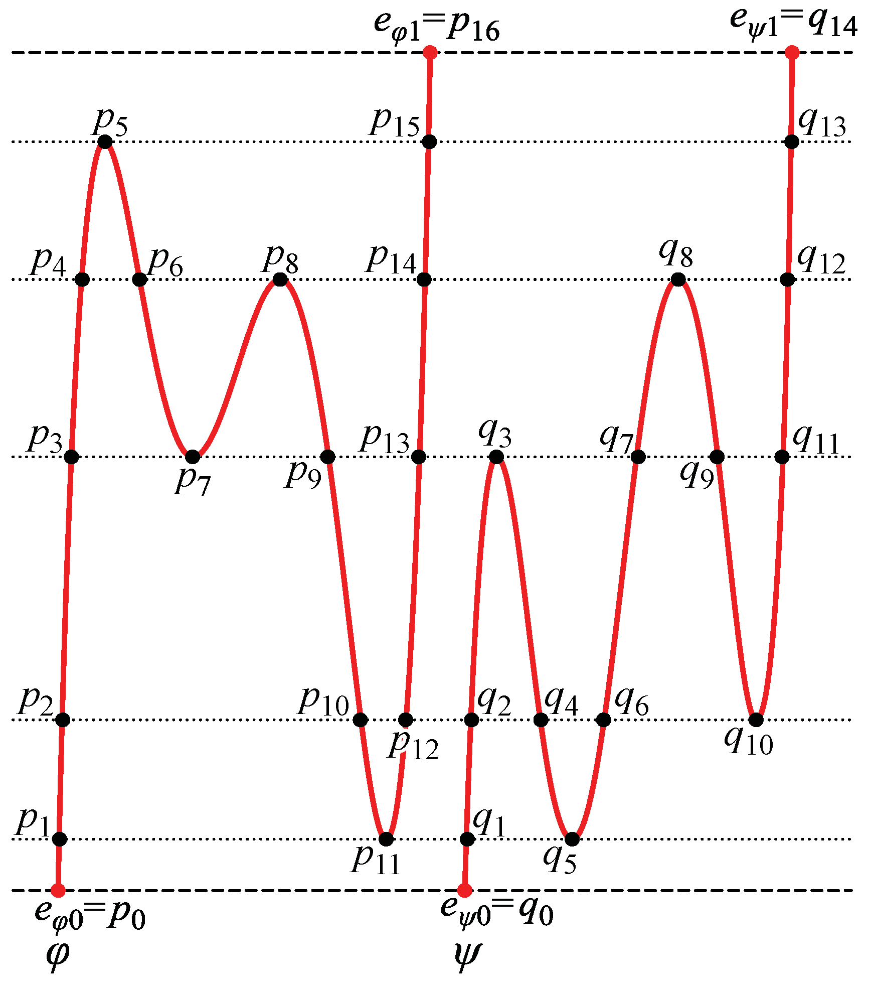
Figure 8. φ and ψ are 2D curves. e_φ0 and e_φ1 are the endpoints of φ, and e_ψ0 and e_ψ1 are the end points of ψ. l₀ is a line connecting e_φ0 and e_ψ0, and l₁ is a line connecting e_φ1 and e_ψ1. l₀ and l₁ are parallel to the x-axis and do not have any intersection with φ and ψ. A line that is parallel to l₀ and intersects with φ has one or more intersections with ψ and vice versa.

Figure 8. φ and ψ are 2D curves. e_φ0 and e_φ1 are the endpoints of φ, and e_ψ0 and e_ψ1 are the end points of ψ. l₀ is a line connecting e_φ0 and e_ψ0, and l₁ is a line connecting e_φ1 and e_ψ1. l₀ and l₁ are parallel to the x-axis and do not have any intersection with φ and ψ. A line that is parallel to l₀ and intersects with φ has one or more intersections with ψ and vice versa.

In order to prove this theorem, we first divide a pair of φ and ψ into multiple pairs of fragments, such that each pair satisfies the assumptions of Theorem 2. Then, we find their backprojections that are mirror-symmetric pairs of continuous curves in the 3D space. Next, we will show that these multiple pairs of 3D curves can share a common symmetry plane Π_s and produce a symmetric pair of continuous curves.

As before we assume that the orientations of the line segments e_φ0e_ψ0 and e_φ1e_ψ1 are horizontal. In this case, e_φ0, e_φ1, e_ψ0 and e_ψ1 are either global maxima or minima of φ and ψ along a vertical axis on the 2D image. Consider horizontal lines that are tangent to the curves at their local extrema (Figure 8). Intersections and tangent points of these horizontal lines with φ and ψ are labeled by numbers sequentially along each curve; p₁, …, p_m on φ and q₁, …, q_n on ψ (in Figure 8, n = 15, and m = 13). Both φ and ψ are divided into segments p₁p₂, p₂p₃ etc. Let the endpoints e_φ0, e_φ1, e_ψ0 and e_ψ1 on φ and ψ be p₀, p_m+1, q₀ and q_n+1, respectively. Let c_φi be a segment of ϕ connecting p_i and its successor p_i+1. Then, c_φi is a curve that is monotonic and continuous between p_i and p_i+1 and these two points are the endpoints of c_φi. Similarly, let c_ψj be a segment of ψ connecting q_j and its successor q_j+1. A segment c_φi of φ has, at least, one corresponding segment of ψ; the endpoints of these segments of ϕ and ψ form parallel line segments. From Theorem 2, a pair of c_φi and each of the corresponding segments of ψ are consistent with an infinite number of 3D symmetric interpretations under an orthographic projection; the one-parameter family of symmetric pairs of 3D curves is characterized by the slant of a symmetry plane. The tilt of the symmetry plane is zero and its depth along the z-axis is arbitrary. It follows that, among all corresponding pairs of 2D segments of these curves, their possible 3D symmetric interpretations can share a common symmetry plane Π_s with some slant σ_s and depth. Hence, φ and ψ are consistent with a one parameter family of symmetric pairs of the 3D fragmented curves that are backprojections of the 2D segments of the 2D curves. In order to prove Theorem 3, we show that, for each member of the family, the symmetric pairs of the 3D fragmented curves produce a symmetric pair of 3D continuous curves whose endpoints are backprojections of the endpoints of φ and ψ. An orthographic projection of such a symmetric pair of the 3D continuous curves will be φ and ψ.

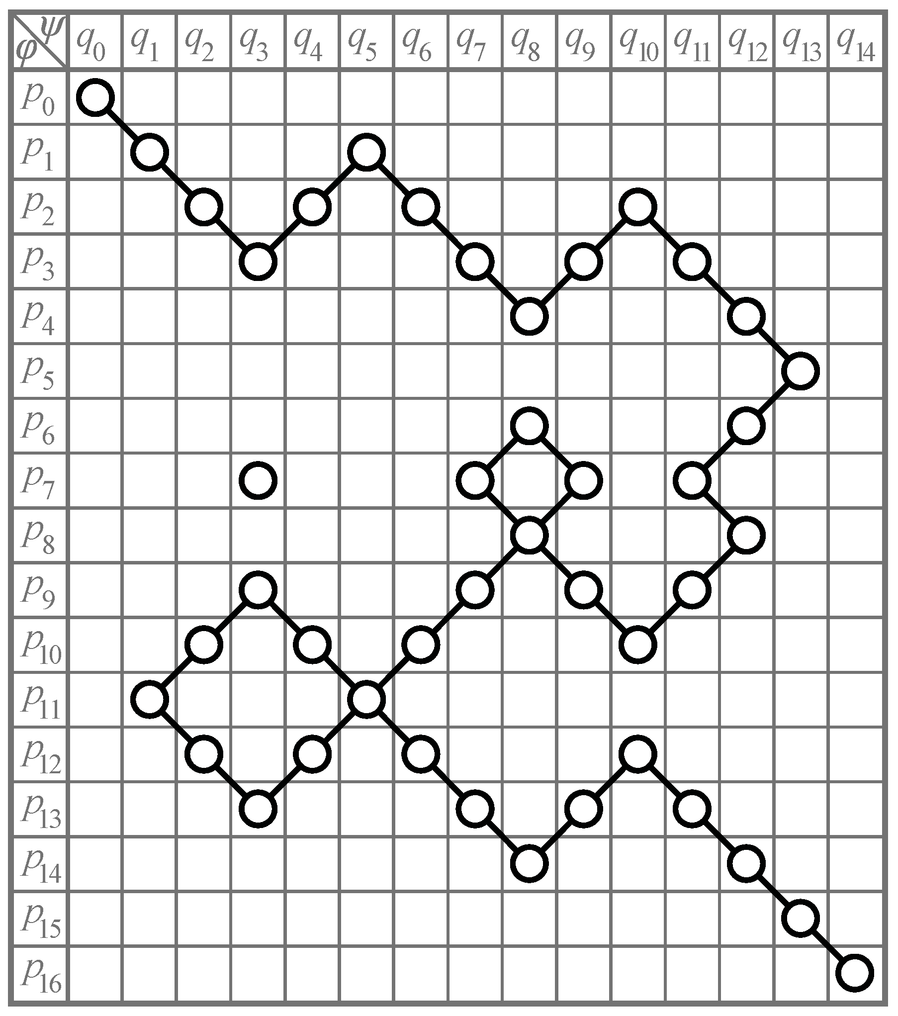
A table representing pairs of the segments of φ and ψ and their endpoints is shown in Figure 9. The rows of the table represent the points p₀, …, p_m+1 on φ. The columns represent the points q₀, …, q_n+1 on ψ. A circle at (p_i, q_j) represents a corresponding pair of points p_i and q_j in Figure 8. These circles are nodes in a graph representing the possible correspondences among pairs of points in Figure 8. Let an edge in this graph connecting (p_i, q_j) and (p_k, q_l) be labeled (p_i, q_j)-(p_k, q_l). Note that the edge (p_i, q_j)-(p_k, q_l) is the same as (p_k, q_l)-(p_i, q_j). The edge (p_k, q_l)-(p_i, q_j) represents a pair of segments of ϕ and ψ, such that c_{φ min(i,k)} connects p_i and p_k and c_{ψ min(j,l)} connects q_j and q_l. Recall that the endpoints of each segment on ϕ and ψ are two neighboring points of φ or ψ; |I − k| = 1 and |j − l| = 1. Hence, an edge in the graph shown in Figure 9 can only connect two nodes that are diagonally next to each other in the table and a node can be connected to, at most, four nodes by four edges. A pair of nodes can be connected to each other only by a single edge. The end nodes of (p_i, q_j)-(p_k, q_l) are either the maxima or minima of these segments and their endpoints form horizontal line segments. Hence, from the Theorem 2, a pair of segments of ϕ and ψ represented by each edge in the graph is consistent with a one-parameter family of pairs of 3D curves that is symmetric with respect to the common symmetry plane Π_s.

Consider two edges (p_i, q_j)-(p_k, q_l) and (p_i, q_j)-(p_g, q_h) connected to a common node (p_i, q_j). These edges represent two pairs of segments of the 2D curves; a pair c_φmin(i,k) and c_ψmin(j,l) and a pair c_φmin(i,g) and c_ψmin(j,h). The two segments c_φmin(i,k) and c_φmin(i,g) are connected to each other at their common endpoint p_i (see Figure 8). In the same way, c_ψmin(j,l) and c_ψmin(j,h) are connected to each other at their common endpoint q_j. Hence, these two pairs of 2D curves can be regarded as a pair of 2D curves whose endpoints are represented by (p_k, q_l) and (p_g, q_h) that are the end nodes of the path formed by the edges. Note that each (p_i, q_j)-(p_k, q_l) and (p_i, q_j)-(p_g, q_h) is consistent with infinitely many pairs of 3D continuous curves. Assume that they are symmetric with respect to the common symmetry plane Π_s whose slant and depth are given. Then, two symmetric pairs of 3D continuous curves are uniquely determined; these 3D curves are backprojections of c_φmin(i,k), c_φmin(i,g), c_ψmin(j,l) and c_ψmin(j,h), respectively. The 3D curves that are backprojections of c_φmin(i,k) and c_φmin(i,g) are connected to each other at their common endpoint that is a backprojection of p_i; these two 3D curves can be regarded as a single 3D curve. The same way, the 3D curves that are backprojections of c_ψmin(j,l) and c_ψmin(j,h) can be regarded as a single 3D curve. It follows that the two symmetric pairs of 3D curves produced from c_φmin(i,k), c_φmin(i,g), c_ψmin(j,l) and c_ψmin(j,h) can be regarded as a single symmetric pair of 3D continuous curves. Their endpoints are backprojections of the 2D points represented by the end nodes (p_k, q_l) and (p_g, q_h) of the continuous path. This can be generalized to all segments of ϕ and ψ as follows. A continuous path of the edges in the table in Figure 9 represents a pair of 2D continuous curves; the 2D curves are composed of the 2D segments of φ and ψ and their endpoints are represented by the end nodes of the path. The 2D curves are consistent with an infinite number of symmetric pairs of 3D continuous curves. The endpoints of the 3D curves are backprojections of the points represented by the end nodes of the path. So, if there is a continuous path connecting (p₀, q₀) and (p_m+1, q_n+1) in the graph in Figure 9, then this path represents a pair of 2D continuous curves φ and ψ and this pair of the 2D curves is consistent with a one-parameter family of symmetric pairs of 3D continuous curves.

The existence of a continuous path of edges connecting (p₀, q₀) and (p_m+1, q_n+1) in the graph will now be proved by using concepts from a graph theory. A graph is called connected if there is a continuous path of edges between every pair of nodes in the graph. If (p₀, q₀) and (p_m+1, q_n+1) belong to a connected graph, there is a path connecting (p₀, q₀) and (p_m+1, q_n+1). A connected graph has even number of nodes of odd degree, where degree of a node refers to number of edges connected to the node [20]. If (p₀, q₀) and (p_m+1, q_n+1) are the only nodes of odd degree in the graph, they must belong to the same connected graph and there must be a continuous path connecting (p₀, q₀) and (p_m+1, q_n+1). Next, we provide a classification of possible nodes in the graph and show that there are only four types: of degree zero, one, two or four. This will conclude the proof.

Consider p₁, …, p_m on φ and q₁, …, q_n on ψ. If a node (p_i, q_j) exists in the table, p_i and q_j form a horizontal line segment in Figure 8. Note that (p_i, q_j) can be connected to, at most, four nodes in the graph that are diagonally next to (p_i, q_j): (p_i−1, q_j−1), (p_i−1, q_j+1), (p_i+1, q_j−1) and (p_i+1, q_j+1). Hence, the maximum degree of each node in the table is four. These four neighboring nodes represent possible pairs of neighboring points of p_i along φ and q_j along ψ. Consider a pair of the neighboring points p_i+1 and q_{j + 1}. The node (p_i+1, q_j+1) exists if and only if p_i+1 and q_j+1 are a corresponding pair; they form a horizontal line segment in Figure 8. Note that p_{i + 1} and p_i are connected by c_φi and q_j+1 and q_j are connected by c_ψj. If both (p_i+1, q_j+1) and (p_i, q_j) exist in the graph, they are connected by (p_i+1, q_j+1)-(p_i, q_j) representing a pair of segments c_φi and c_ψj. Therefore, the number of edges in the graph connected to (p_i, q_j) can be computed by verifying the existence of the four neighboring nodes.

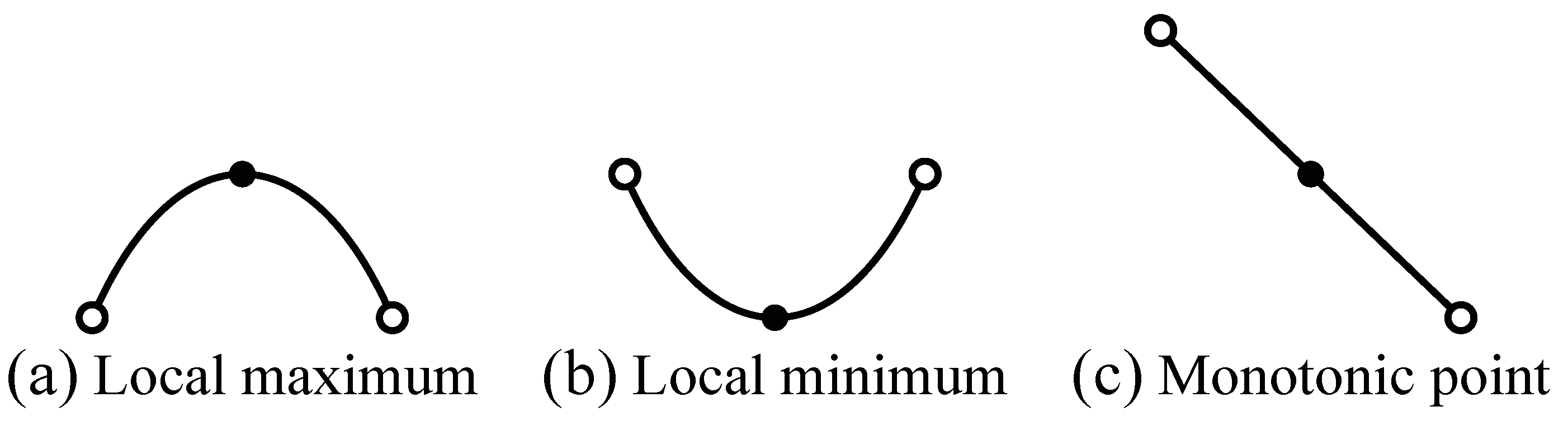
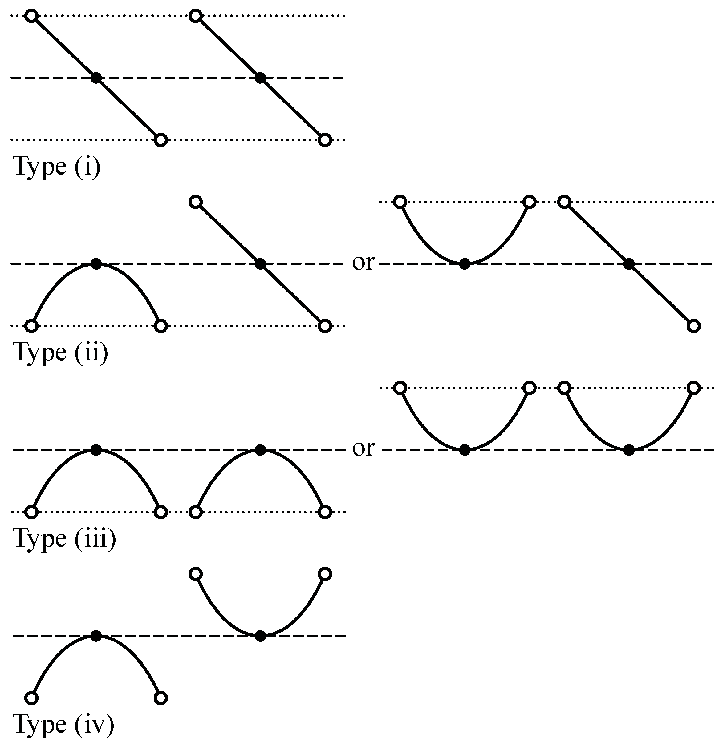
In order to compute the number of edges connected to each node, points and corresponding pairs of points represented by the nodes in the graph are classified. Consider points p₁, …, p_m and q₁, …, q_n. First, these points can be classified into three types: local maxima, local minima and points at which the curve is monotonic (Figure 10). If a point is a local maximum, its neighboring points are lower than the local maximum. If a point is a local minimum, its neighboring points are higher than the local minimum. If a point is a “monotonic point”, one of its neighboring points is higher and the other is lower. Next, based on the classification of the points, the corresponding pairs of the points can be classified into three types (Figure 11). Type (i): if two monotonic points are corresponding, a node representing this pair of points is connected to two nodes by two edges. Hence, the degree of this node is two; Type (ii): if a monotonic point and a local maximum/minimum are corresponding, the degree of a node representing this pair is also two; Type (iii): if two local maxima/minima are corresponding, the degree of a node representing this pair is four; Type (iv): if a local maximum and a local minimum are corresponding, the degree of a node representing this pair is zero. From these facts, the degree of any node which does not represent the endpoints of the two curves is always even (0, 2 or 4).

Next, consider pairs of endpoints of φ and ψ: (p₀, q₀) and (p_{m + 1}, q_n+1). Recall that p₀ = e_φ0, p_m+1 = e_φ1, q₀ = e_ψ0 and q_n+1 = e_ψ1; so, the line segments p₀q₀ and p_m+1q_n+1 are horizontal in Figure 8. Hence, these pairs of the endpoints are corresponding pairs and the nodes representing these pairs exist in the graph. Note that these endpoints are global maxima and minima of φ and ψ; the global maxima form a corresponding pair and the global minima form a corresponding pair. Recall that if two local maxima or two local minima form a corresponding pair, there are four corresponding pairs of their neighboring points. However, each endpoint has only one neighboring point. Hence, there is one corresponding pair of the neighboring points for each pair of the endpoints. Therefore, each (p₀, q₀) and (p_m+1, q_n+1) is connected to a single node and their degrees are one, which is an odd number.

Note that the case where φ or ψ has a local extremum at which a horizontal line connecting e_φ0 and e_ψ0 or e_φ1 and e_ψ1 is tangent to the curve of the extremum, is analogous to Type (ii) in Figure 11. The extremum of the curve corresponds to an endpoint of the other curve that is on the horizontal tangent line. Unlike Type (ii), the endpoint has only one neighboring point that forms a corresponding pair with the neighboring points of the local extremum. Hence, the degree of a node representing the pair of the local extremum and the endpoint is also two, which is an even number.

From these facts, there are two nodes (p₀, q₀) and (p_m+1, q_n+1) whose degrees are odd (1) and the degrees of all other nodes are even (0, 2 or 4). Hence, (p₀, q₀) and (p_m+1, q_n+1) must belong to the same connected graph and these two nodes are connected by a continuous path of edges. This continuous path in the graph represents the correspondences between 3D continuous curves of a symmetric pair whose orthographic projections are the 2D curves φ and ψ, respectively. Once the correspondences are formed, the pair of the 3D curves can be produced using Equations (15) and (16). Note that the slant of the symmetry plane Π_s is a free parameter of the 3D symmetric interpretation of φ and ψ under an orthographic projection. A symmetric pair of 3D curves produced from the pair of 2D curves in Figure 8 is shown in Demo 6 in supplemental material [2].

This proof of Theorem 3 for an orthographic projection can be easily generalized to the case of a perspective projection:

Theorem 4:

Let φ and ψ be curves that are tame in a single 2D image. Let the endpoints of φ be e_φ0 and e_φ1, and the endpoints of ψ be e_ψ0 and e_ψ1. Let a line connecting e_φ0 and e_ψ0 be l₀ and that connecting e_φ1 and e_ψ1 be l₁. Assume that φ and ψ have the following properties: (i) l₀ and l₁ intersect at a point v that is not on φ or ψ; (ii) l₀ and l₁ do not have any intersection with φ and ψ; (iii) v is not between e_φ0 and e_ψ0 or between e_φ1 and e_ψ1; and (iv) a half line that emanates from v and intersects with φ has one or a finite number of intersections with ψ and vice versa. Then, there exists a pair of continuous curves Φ and Ψ and a plane Π_s in a 3D space for a given center of projection F, such that Φ and Ψ are mirror-symmetric with respect to Π_s and that φ is a perspective projection of Φ and ψ is a perspective projection of Ψ.

Proof: In the proof of Theorem 3 for the case of an orthographic projection, the 2D curves φ and ψ were divided by lines which were parallel to e_φ0e_ψ0 and were tangent to either of the 2D curves. In the case of a perspective projection, φ and ψ are divided by lines which emanate from the vanishing point v and are tangent to either of the 2D curves. The rest of this proof is identical to that of Theorem 3. The only difference is that in the case of a perspective projection the 3D interpretation is unique—the slant of the symmetry plane is not a free parameter.

In the four theorems above it was assumed that an endpoint of one curve corresponds to an endpoint of the other curve. Next, we generalize Theorems 3 and 4 to the case where an endpoint of a curve may or may not correspond to an endpoint of the other curve. This can happen, for example, in the presence of occlusion. We begin with the case of an orthographic projection.

Theorem 5:

Let φ and ψ be curves that are tame in a 2D image. Assume that there exist two lines l₀ and l₁ which satisfy the following properties: (i) l₀ and/or l₁ is either tangent to both φ and ψ or passes through their endpoints, (ii) l₀||l₁, (iii) l₀ and l₁ do not have any intersection with φ and ψ and (iv) a line that is parallel to l₀ and intersects φ has one or a finite number of intersections with ψ and vice versa (see Figure 12). Then, there exist infinitely many pairs of continuous curves Φ and Ψ and a plane Π_s in a 3D space, such that Φ and Ψ are mirror-symmetric with respect to Π_s and that φ is an orthographic projection of Φ and ψ is an orthographic projection of Ψ.

In order to prove this theorem, we first extend φ and ψ and obtain a pair of 2D curves φ′ and ψ′ that perfectly overlap φ and ψ in the 2D image and satisfy the assumptions of Theorem 3. Then, we find the backprojections of φ′ and ψ′ in the 3D space, such that these backprojected curves are mirror-symmetric with respect to a plane Π_s. Their orthographic projections in the 2D image coincide with φ′ and ψ′, as well as with φ and ψ.

Let the orientations of l₀ and l₁ be horizontal. In this case, tangent points of φ and ψ to l₀ or l₁ are either global maxima or minima of φ and ψ along a vertical axis on the 2D image. Assume that the endpoints of these curves are not global extrema—the case when they are global extrema has been considered in the previous theorems. Let the tangent points of φ to l₀ and l₁ be t_φ0 and t_φ1. Let an endpoint of φ, which is closer (as measured by the arc length along the curve) to t_φ0 be e_φ0, and that, which is closer to t_φ1 be e_φ1. The same way, let the tangent points of ψ to l₀ or l₁ be t_ψ0 and t_ψ1, and the endpoints ψ be e_ψ0 and e_ψ1.

We extend the 2D curves φ and ψ by adding arcs that start from e_φ0, e_φ1, e_ψ0 and e_ψ1, which are endpoints of φ and ψ. The extension starting from e_φ0 is identical to the segment of φ between e_φ0 and t_φ0. Similarly, the extension starting from e_φ1 is identical to the segment of φ between e_φ1 and t_φ1. Let this new curve be φ′. Let the endpoints of φ′ be e′_φ0 and e′_φ1, so that the positions of e′_φ0 and e′_φ1 are respectively the same as those of t_φ0 and t_φ1 in the 2D image. The same way, let the extended curve produced from ψ be ψ′ and the endpoints of ψ′ be e′_ψ0 and e′_ψ1. The positions of e′_ψ0 and e′_ψ1 are respectively the same as those of t_ψ0 and t_ψ1 in the 2D image. The curves φ′ and ψ′ perfectly overlap φ and ψ in the 2D image (Figure 12). Therefore, the 3D interpretations of φ′ and ψ′ are also consistent with the 3D interpretations of φ and ψ. It is easy to see that φ′ and ψ′ satisfy the assumptions of Theorem 3. Therefore, it follows from the proof of Theorem 3 that there exists a one-parameter family of symmetric pairs of continuous 3D curves Φ′ and Ψ′, such that φ′ is an orthographic projection of Φ′ and ψ′ is an orthographic projection of Ψ′. This, in turn, implies that φ and ψ are also orthographic projection of Φ′ and Ψ′. A symmetric pair of 3D curves produced from the pair of 2D curves in Figure 12 is shown in Demo 7 in supplemental material [2] (It looks like each of the 3D curves in Demo 6 has four endpoints, rather than two, as would be expected from Theorem 3. It also looks like each of the 3D curves has two bifurcations. All of the four points that look like endpoints are actually 180° turns of the 3D curve. The real endpoints of the 3D curve are at the bifurcations).

Proof:

Figure 12. φ and ψ (red solid curves) are 2D curves. e_φ0 and e_φ1 are the endpoints of φ, and e_ψ0 and e_ψ1 are the end points of ψ. l₀ is tangent to both φ and ψ at t_φ0 and t_ψ0, and l₁ is tangent to both φ and ψ at t_φ1 and t_ψ1. l₀ and l₁ are parallel to the x-axis and do not have any intersection with φ and ψ. The two curves, φ and ψ are extended by adding arcs (blue dotted curves) that start from e_φ0, e_φ1, e_ψ0 and e_ψ1. The additional arcs are identical to the segments of φ and ψ (note that the blue dotted curves are perfectly overlapping the red solid curves in the image). They end at e′_φ0, e′_φ1, e′_ψ0 and e′_ψ1 whose positions are respectively the same as those of t_φ0, t_φ1, t_ψ0 and t_ψ1. See Demo 7 in supplemental material for an interactive illustration of the 3D symmetric curves produced from φ and ψ [2].

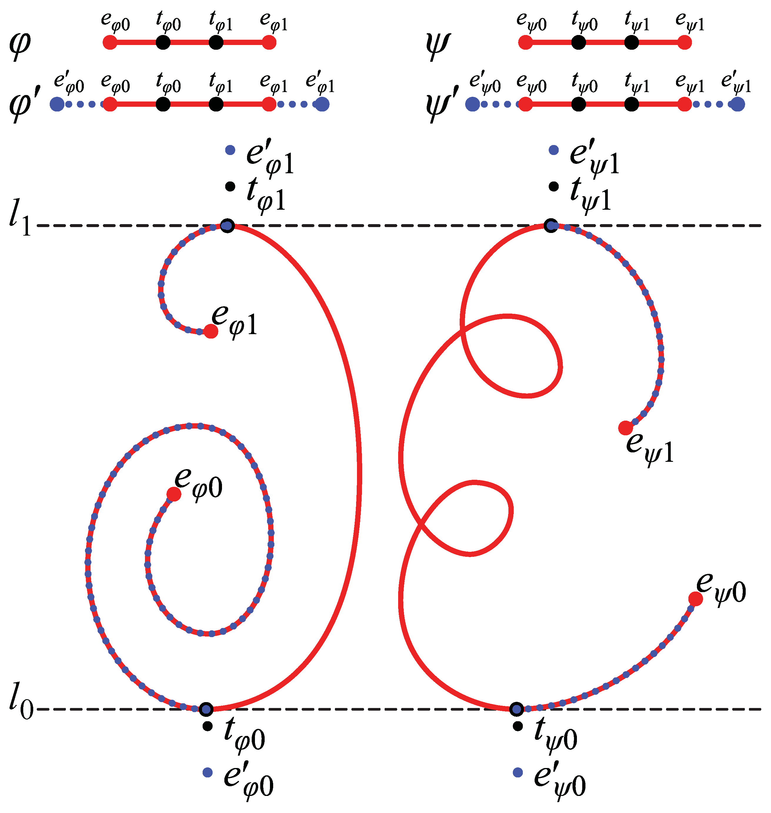
Figure 12. φ and ψ (red solid curves) are 2D curves. e_φ0 and e_φ1 are the endpoints of φ, and e_ψ0 and e_ψ1 are the end points of ψ. l₀ is tangent to both φ and ψ at t_φ0 and t_ψ0, and l₁ is tangent to both φ and ψ at t_φ1 and t_ψ1. l₀ and l₁ are parallel to the x-axis and do not have any intersection with φ and ψ. The two curves, φ and ψ are extended by adding arcs (blue dotted curves) that start from e_φ0, e_φ1, e_ψ0 and e_ψ1. The additional arcs are identical to the segments of φ and ψ (note that the blue dotted curves are perfectly overlapping the red solid curves in the image). They end at e′_φ0, e′_φ1, e′_ψ0 and e′_ψ1 whose positions are respectively the same as those of t_φ0, t_φ1, t_ψ0 and t_ψ1. See Demo 7 in supplemental material for an interactive illustration of the 3D symmetric curves produced from φ and ψ [2].

This proof of Theorem 5 for an orthographic projection can be easily generalized to the case of a perspective projection, the same way as the proof of Theorem 3 was generalized to the case of perspective projection:

Theorem 6:

Let φ and ψ be curves that are tame in a 2D image. Assume that there exist two lines l₀ and l₁ which satisfy the following properties: (i) l₀ and/or l₁ is either tangent to both φ and ψ or passes through their endpoints; (ii) l₀ and l₁ intersect at a point v that is not on φ or ψ; (iii) l₀ and l₁ do not have any other intersections with φ and ψ; (iv) v is not between e_φ0 and e_ψ0 or between e_φ1 and e_ψ1, and (v) a half line that emanates from v and intersects with φ has one or a finite number of intersections with ψ and vice versa. Then, there exists a pair of continuous curves Φ and Ψ and a plane Π_s in a 3D space for a given center of projection F, such that Φ and Ψ are mirror-symmetric with respect to Π_s and that φ is a perspective projection of Φ and ψ is a perspective projection of Ψ.

3. Discussion

In this paper, we showed that any pair of 2D curves that are sufficiently regular is consistent with a 3D symmetric interpretation under quite general assumptions. We derived the equations that allow one to compute the 3D curves for the case of perspective and orthographic projections. Although the main part of the proofs is fairly straightforward, the result is surprising and has important implications for theories of shape perception.

Consider the examples in Figure 1, Figure 2, Figure 3, Figure 5, Figure 7, Figure 8 and Figure 13. Although these pairs of 2D curves do not look like symmetric pairs of 3D curves, they do have 3D symmetric interpretations. What is the nature of the process that can produce 3D symmetry from an arbitrary 2D image? The key element of this process seems to be related to the concept of degenerate views. Essentially, the 3D viewing direction for which the 3D symmetric curves project to the given 2D asymmetric curves is degenerate and the 3D symmetry becomes “hidden” in the 2D image. There are two cases representing a degenerate view. The first, more obvious case, happens when multiple segments of a 3D curve project to the same segment of a 2D curve. This can be seen in the 3D symmetric interpretations of Figure 7, Figure 8 and Figure 13 (see Demos 5–7 [2]). The second, more subtle case, corresponds to the situation where a local curvature of a 3D curve disappears in the 2D projection. The simplest example is when a planar curve in the 3D space projects to a straight line segment in the 2D image [21]. However, if a curve in the 3D space is not planar, then its 2D projection is never a straight line segment, even for degenerate views. Recall that curvature of a 3D curve (also called first curvature) represents the change of the tangent to the curve within the plane of the circle of curvature, while torsion (also called second curvature) represents the change of the tangent to the curve away from the plane of the circle of curvature [22]. If the normal of the plane of the circle of curvature is perpendicular to the line of sight, the change of the tangent within this plane (i.e., curvature of the 3D curve) disappears in the 2D projection, but the departure from this plane (i.e., torsion of the 3D curve) does not. In a sense, for such views, the local curvature of a 2D curve is a projection of the local torsion of a 3D curve. Figure 2, Figure 3 and Figure 5 illustrate the second case of degenerate views (see Demos 2–4 [2]). Apparently, the visual system “rejects” 3D symmetric interpretations if they imply degenerate views. This makes sense because degenerate views are unlikely.

Perhaps the simplest way to reduce the possibility of degenerate views in 3D interpretations is to impose a constraint that the 3D curves are planar [23]. A planar 3D curve will produce a degenerate view if and only if the 3D curve projects to a straight line in the 2D image (this case is easy to detect and exclude). Preliminary experiments showed that this constraint captures some aspects of human perception of a 3D shape [6,10,24]. This observation is illustrated in Figure 13 (Figure 13a is identical to Figure 1). When two planar curves are mirror symmetric in 3D, their orthographic projections are related by a 2D affine transformation, with an additional constraint that the line segments connecting pairs of corresponding points are parallel. Such an image is shown in Figure 13a and its symmetric interpretation is shown in Figure 13b (see also Demo 8 in supplemental material for an interactive illustration of the 3D symmetric curve [2]). Here we show a 2D closed curve, which is an orthographic image of a mirror-symmetric 3D closed curve. In order to apply our theorems, we split the 2D closed curve into two open curves at top and bottom corners of the curve. The relation between these two open curves is a 2D affine stretching transformation along horizontal direction. The 3D symmetric interpretation shown in Figure 13b was produced by using the “correct” correspondences, in which pairs of corresponding points form horizontal line segments. Each of the two symmetric halves of this 3D interpretation is a planar curve (see Demo 8). The reader surely perceives a 3D symmetric curve when looking at Figure 13a and this perceptual interpretation is close to the 3D symmetric interpretation derived from our theorems (see Figure 13b and Demo 8 [2]).

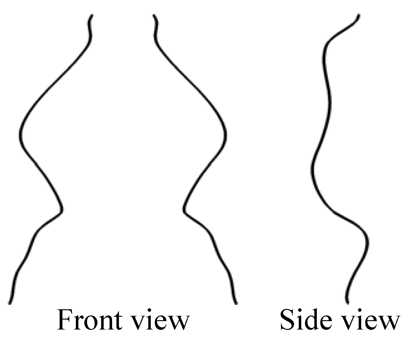
Figure 13. A 2D closed curve and its two different symmetric interpretations. (a) An orthographic projection of a closed symmetric curve. Each of the two symmetric halves of the curve is planar. The corresponding pairs of the points of the curve form horizontal line segments; (b) The front view of the symmetric interpretation of the curve in (a) using the “correct” correspondence. The slant and the tilt of the symmetry plane of the symmetric interpretation were set to 40° and 0°, respectively. Each of the two symmetric halves of the 3D curve is planar; (c) The front view of the symmetric interpretation of the curve in (a) using the “wrong” correspondence. The slant and the tilt of the symmetry plane were set to 40° and −25°, respectively. Neither of the two symmetric halves of the 3D curve is planar. See Demo 8 in supplemental material for an interactive illustration showing these two different 3D curves produced from the same 2D image [2].

Figure 13. A 2D closed curve and its two different symmetric interpretations. (a) An orthographic projection of a closed symmetric curve. Each of the two symmetric halves of the curve is planar. The corresponding pairs of the points of the curve form horizontal line segments; (b) The front view of the symmetric interpretation of the curve in (a) using the “correct” correspondence. The slant and the tilt of the symmetry plane of the symmetric interpretation were set to 40° and 0°, respectively. Each of the two symmetric halves of the 3D curve is planar; (c) The front view of the symmetric interpretation of the curve in (a) using the “wrong” correspondence. The slant and the tilt of the symmetry plane were set to 40° and −25°, respectively. Neither of the two symmetric halves of the 3D curve is planar. See Demo 8 in supplemental material for an interactive illustration showing these two different 3D curves produced from the same 2D image [2].

The 3D symmetric interpretation in Figure 13c was produced by using “wrong” correspondences. The correspondences were established here by using lines forming an angle of 25° with the horizontal line (clockwise). Each of the two symmetric halves of this 3D interpretation is a non-planar curve (see Demo 8). Clearly, the reader does not perceive this 3D interpretation when looking at Figure 13a. The examples shown in Figure 13 and Demo 8 suggest that the reason for why the human visual system uses planarity constraint is not the fact that planar curves are common in the natural 3D environment (which may very well be true, see [19]), but that planar (or close to planar) interpretations are rarely associated with degenerate views, and, therefore, are more likely.

These observations lead us to the conclusion that there may be at least three ways of excluding spurious (incorrect) 3D symmetric interpretations when 3D shape recovery is performed from a single 2D retinal image: The first one is to perform 3D recovery and verify whether the corresponding 3D view is degenerate and thus unlikely. The second one is to impose a planarity constraint on 3D recovery. The third one is to establish contour-configural organization in the 2D image before 3D shape recovery is performed. Specifically, the visual system may detect higher order features such as corners, junctions and regions. Once such features are detected, one can establish their correspondence using similarity. For example, sharp corners in one contour are likely to correspond to sharp contours in another one [25]. Recall that the human visual system is extremely sensitive to corners: the ability to discriminate between a straight line segment and a corner belongs to what is referred to as “hyperacuity” in the human visual system, which refers to visual discriminations that are done at “sub-pixel” resolution [26]. Once the plausible correspondence is established, one can verify whether the lines connecting pairs of corresponding features are parallel (or intersect at a single point). If they are not, a 3D symmetric interpretation does not exist.

We want to emphasize that the actual mechanisms used by the human visual system are still largely unknown. What is known at this point is that human observers can very reliably discriminate between 3D symmetric and asymmetric shapes based on a single 2D non-degenerate image of a 3D polyhedron [9,10]. Note that polyhedral objects are composed of (i) planar faces, (ii) edges and (iii) corners. All three are distinctive higher order features that can be used to establish correct correspondences. Hence, it is possible to reliably verify whether a 3D symmetric interpretation exists for a non-degenerate 2D image of a polyhedron. In fact, one of us formulated a computational model of such discrimination [10]. Performance of this model is as good as the performance of the subjects. The model, besides using the correct correspondences (that was assumed to be known), applied a weighted combination of the following constraints: symmetry of a 3D shape, planarity of faces, maximal 3D compactness and minimum surface area. It turns out that the models (and the subjects) visually “prefer” a 3D asymmetric interpretation whose 3D compactness is large and whose faces are planar, rather than a 3D symmetric interpretation whose 3D compactness is small and/or some faces are not planar. It follows that symmetry is not the only constraint operating in human vision, but quite possibly it should be regarded as the most fundamental constraint because (i) symmetry is universal in nature, and (ii) symmetry constraint reduces the family of possible 3D interpretation the most.

Finally, we want to point out that our theoretical result presented in this paper may put some limitations on the generality of Leyton’s [27] theory of shape perception. According to Leyton, a shape is perceived and memorized by removing the asymmetry from the image that is a 2D projection of a 3D symmetric shape. This process of symmetrization, which closely resembles Pierre Curie’s symmetry principle [28], was expected to correctly recover the 3D symmetric shape. However, since 3D symmetric interpretations exist for every 2D image, including images of an asymmetric 3D shape, one can never be sure whether the recovered 3D symmetry is the correct 3D interpretation. Clearly, 3D recovery in human and computer vision must be treated as an ill-posed inverse problem, whose solution involves tools of a regularization theory or Bayesian inference [1,29,30]. When inverse problems are solved by the human visual system, the retinal information is combined with a priori constraints, and symmetry is only one of several constraints that are being used by the visual system.

References and Notes

- Pizlo, Z. 3D Shape: Its Unique Place in Visual Perception; MIT Press: Cambridge, MA, USA, 2008. [Google Scholar]
- Our online demos are available at: http://www.psych.purdue.edu/~zpizlo/sym2011/ (also available as a supplementary material accompanying the online article).
- Hochberg, J.; Brooks, V. Pictorial recognition as an unlearned ability: A study of one child’s performance. Am. J. Psychol. 1962, 75, 624–628. [Google Scholar] [CrossRef] [PubMed]
- Koenderink, J.J.; van Doorn, A.J.; Christou, C.; Lappin, J.S. Shape constancy in pictorial relief. Perception 1996, 25, 155–164. [Google Scholar] [CrossRef] [PubMed]
- Li, Y.; Pizlo, Z. Depth cues vs. simplicity in 3D shape perception. Top. Cogn. Sci. 2011. submitted. [Google Scholar]
- Chan, M.W.; Stevenson, A.K.; Li, Y.; Pizlo, Z. Binocular shape constancy from novel views: The role of a priori constraints. Percept. Psychophys. 2006, 68, 1124–1139. [Google Scholar] [CrossRef] [PubMed]
- Li, Y.; Pizlo, Z. Reconstruction of shapes of 3D symmetric objects by using planarity and compactness constraints. In Proceedings of the SPIE/IS&T Electronic Imaging Symposium, Conference on Vision Geometry, San Jose, CA, USA, January 2007; Volume 6499, pp. 64990B1–64990B10. [Google Scholar]
- Li, Y.; Pizlo, Z.; Steinman, R.M. A computational model that recovers the 3D shape of an object from a single 2D retinal representation. Vis. Res. 2009, 49, 979–991. [Google Scholar] [CrossRef] [PubMed]
- Sawada, T.; Pizlo, Z. Detecting mirror-symmetry of a volumetric shape from its single 2D image. In Proceedings of the 6th IEEE Computer Society Workshop on Perceptual Organization in Computer Vision, Anchorage, AK, USA, June 2008. [Google Scholar]
- Sawada, T. Visual detection of symmetry of 3D shapes. J. Vis. 2010, 10, 1–22. [Google Scholar] [CrossRef] [PubMed]
- Pizlo, Z.; Sawada, T.; Li, Y.; Kropatsch, W.G.; Steinman, R.M. New approach to the perception of 3D shape based on veridicality, complexity, symmetry and volume. Vis. Res. 2010, 50, 1–11. [Google Scholar] [CrossRef] [PubMed]
- Steiner, G. Spiegelsymmetrie der tierkörper. Naturwiss. Rundsch. 1979, 32, 481–485. [Google Scholar]
- Vetter, T.; Poggio, T. Symmetric 3D objects are an easy case for 3D object recognition. Spat. Vis. 1994, 8, 443–453. [Google Scholar] [PubMed]
- François, A.R.J.; Medioni, G.G.; Waupotitsch, R. Mirror symmetry→2-view stereo geometry. Image Vis. Comput. 2003, 21, 137–143. [Google Scholar] [CrossRef]
- Gordon, G.G. Shape from symmetry. In Proceedings of the SPIE Conference, Intelligent Robots and Computer Vision VIII: Algorithms and Techniques, Philadelphia, PA, USA, November 1989; Volume 1192, pp. 297–308. [Google Scholar]
- Rothwell, C.A. Object Recognition through Invariant Indexing; Oxford University Press: Oxford, UK, 1995. [Google Scholar]
- Yang, A.Y.; Huang, K.; Rao, S.; Hong, W.; Ma, Y. Symmetry-based 3-D reconstruction from perspective images. Comput. Vis. Image Underst. 2005, 99, 210–240. [Google Scholar] [CrossRef]
- Latecki, L.J.; Rosenfeld, A. Supportedness and tameness: Differentialless geometry of plane curves. Pattern Recogn. 1998, 31, 607–622. [Google Scholar] [CrossRef]
- Hong, W.; Ma, Y.; Yu, Y. Reconstruction of 3-D deformed symmetric curves from perspective images without discrete features. Lect. Notes Comput. Sci. 2004, 3023, 533–545. [Google Scholar]
- Thulasiraman, K.; Swamy, M.N.S. Graphs: Theory and Algorithms; Wiley: New York, NY, USA, 1992. [Google Scholar]
- Mach, E. The Analysis of Sensations and the Relation of the Physical to the Psychical; Dover: New York, NY, USA, 1959. [Google Scholar]
- Hilbert, D.; Cohn-Vossen, S. Geometry and the Imagination; Chelsea Publishing Company: New York, NY, USA, 1952. [Google Scholar]
- Barrow, H.G.; Tenenbaum, J.M. Interpreting line drawings as three-dimensional surfaces. Artif. Intell. 1981, 17, 75–116. [Google Scholar] [CrossRef]
- Pizlo, Z.; Stevenson, A.K. Shape constancy from novel views. Percept. Psychophys. 1999, 61, 1299–1307. [Google Scholar] [CrossRef] [PubMed]
- Yuen, S.Y.K. Shape from contour using symmetries. Lect. Notes Comput. Sci. 1990, 427, 437–453. [Google Scholar]
- Watt, R.J. Towards a general theory of the visual acuities for shape and spatial arrangement. Vis. Res. 1984, 24, 1377–1386. [Google Scholar] [CrossRef]
- Leyton, M. Symmetry, Causality, Mind; MIT Press: Cambridge, MA, USA, 1992. [Google Scholar]
- Curie, P. On symmetry in physical phenomena, symmetry of an electric field and of a magnetic field. J. Phys. 1894, 3, 395–415. [Google Scholar]
- Poggio, T.; Torre, V.; Koch, C. Computational vision and regularization theory. Nature 1985, 317, 314–319. [Google Scholar] [CrossRef] [PubMed]
- Pizlo, Z. Perception viewed as an inverse problem. Vis. Res. 2001, 41, 3145–3161. [Google Scholar] [CrossRef]
Figure 1.
A 2D closed curve that looks like a 2D projection of a 3D mirror-symmetric curve. See Demo 1 in supplemental material for an interactive illustration of the 3D symmetric interpretation produced from this 2D curve [2].
Figure 2.
An asymmetric pair of 2D curves and the 3D symmetric interpretation. (a) An asymmetric pair of 2D curves. These curves can be interpreted as a 2D perspective projection of a symmetric pair of 3D curves whose symmetry plane is slanted at an angle of 40° (see Theorem 1); (b) Three different views of the 3D symmetric interpretation produced from the pair of the 2D curves in (a). The numbers in the bottom are the values of the slant σs of the symmetry plane of the symmetric pair of the 3D curves. For σs equal to 40°, the image is identical to that in (a). When σs is 90°, its 2D projection itself becomes symmetric. See Demo 2 in supplemental material for an interactive illustration of the 3D symmetric curves [2].
Figure 4.
Front and side views of a symmetric pair of 3D curves produced from the pair of 2D curves in Figure 3. The distance zf between the center of projection and the image plane, together with the vanishing point v determine the slant σs of the symmetry plane Πs (the slant is 30° in this case). See Demo 3 in supplemental material for an interactive illustration of the 3D symmetric curves [2]. Note that a perspective projection is used in Demo 3. As a result, the two curves in the side view do not project to the same curve on the image: the farther curve projects to a smaller image. The side view in this figure was computed using an orthographic projection. As a result, the two symmetric 3D curves project to the same 2D image.
Figure 6.
Views of a symmetric pair of 3D curves produced from the pair of 2D curves in Figure 5. The slant σs of the symmetry plane Πs was set to 45°. See Demo 4 in supplemental material for an interactive illustration of the 3D symmetric curves [2].
Figure 9.
This table represents pairs of segments and pairs of points on of ϕ and ψ. The rows represent the points p0, …, pm+1 on φ. The columns represent the points q0, …, qn+1 on ψ. A circle at (pi, qj), which is a node in the graph, represents a corresponding pair of points pi and qj; pi and qj form a horizontal line segment in Figure 8. The top left and bottom right nodes represent pairs of endpoints of φ and ψ. An edge (pi, qj)-(pk, ql) (or (pk, ql)-(pi, qj)) connecting (pi, qj) and (pk, ql) represents a pair of segments of ϕ and ψ.
Figure 10.
Three types of points (solid circles) on a 2D curve and their neighboring points (open circles).
Figure 11.
Four types of pairs of points (solid circles) and their neighboring points (open circles). See text for more information.
© 2011 by the authors. Licensee MDPI, Basel, Switzerland. This article is an open access article distributed under the terms and conditions of the Creative Commons Attribution (CC BY) license (http://creativecommons.org/licenses/by/4.0/).
Share and Cite
MDPI and ACS Style
Sawada, T.; Li, Y.; Pizlo, Z. Any Pair of 2D Curves Is Consistent with a 3D Symmetric Interpretation. Symmetry 2011, 3, 365-388. https://doi.org/10.3390/sym3020365
AMA Style
Sawada T, Li Y, Pizlo Z. Any Pair of 2D Curves Is Consistent with a 3D Symmetric Interpretation. Symmetry. 2011; 3(2):365-388. https://doi.org/10.3390/sym3020365
Chicago/Turabian StyleSawada, Tadamasa, Yunfeng Li, and Zygmunt Pizlo. 2011. "Any Pair of 2D Curves Is Consistent with a 3D Symmetric Interpretation" Symmetry 3, no. 2: 365-388. https://doi.org/10.3390/sym3020365