Maniplexes: Part 1: Maps, Polytopes, Symmetry and Operators ^†

Abstract

This paper introduces the idea of a maniplex, a common generalization of map and of polytope. The paper then discusses operators, orientability, symmetry and the action of the symmetry group.

1. Introduction

The primary purpose of this paper is to introduce the idea of a maniplex. This notion generalizes the idea of map to higher dimensions, while at the same time slightly generalizing (and perhaps simplifying) the idea of abstract polytope.

Part of the motivation for proposing these definitions is the desire to unify the topics of Map and Polytope, to demonstrate their similarity and commonalities.

We will first give definitions for map and (abstract) polytope. We will compare and contrast the two notions. The two topics have in common two simple ideas. One is the idea of a flag being the unit brick of construction. The other is that we make items of one dimension by assembling items of one dimension less. We define maniplex to generalize both. We then discuss: (1) operators which make one maniplex from another; (2) orientability, symmetry and the action of the symmetry group.

A sequel to this paper will deal with (3) the idea of consistent cycles in graphs (see [1,2]) and its applications to maps, polytopes and maniplexes, and (4) a construction which expands the possibilities for semisymmetric graphs as medial layer graphs (see [3,4]).

First, we examine the foundations of both maps and polytopes.

2. Maps

We begin by defining a map $\mathcal{M}$ to be an embedding of a connected graph into a compact connected surface. Beneath the apparent simplicity of this definition lie a number of caveats of two types: We are being loose about the word “graph” and restrictive about “embedding”.

First, when we use the word “graph”, we include what some sources call “multigraphs” or “pseudographs”. In particular, we allow such aberrations as loops, multiple edges and semi-edges. Secondly, we want an “embedding” to be a continuous, one-to-one function from a topological form of a graph into a surface which is nice in several ways: (1) the image of the interior of each edge has a neighborhood which is homeomorphic to a disk; (2) each connected component of the complement of the image of the graph is itself homeomorphic to a disk. This is sometimes called a “cellular embedding”. We can then think of the cube as an embedding of a graph of eight trivalent vertices onto the sphere. Maps exist on all surfaces.

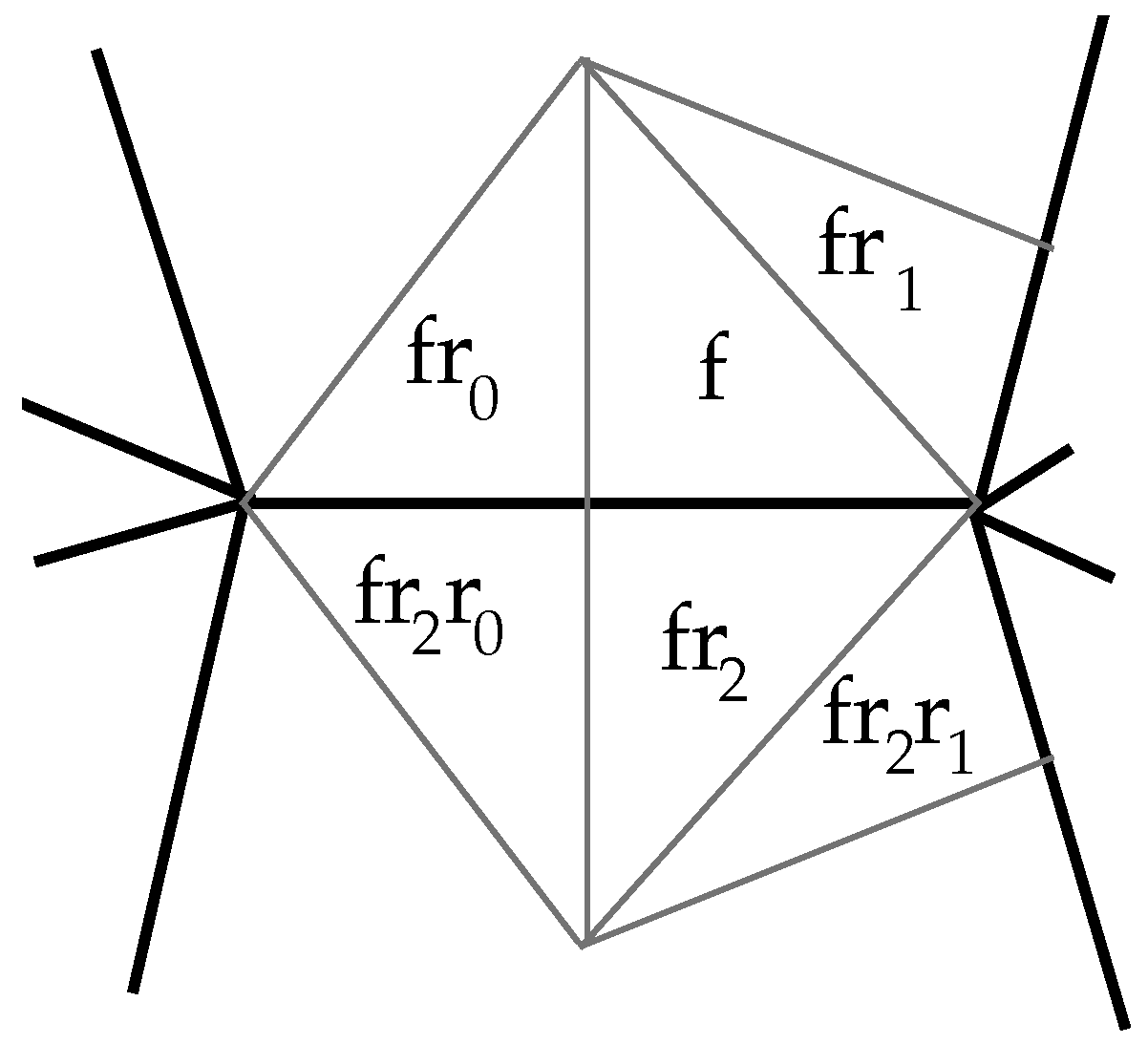
How can we think of a map combinatorially? Our first step is to choose some point in the interior of each face to be its “center”. We choose a point in the (relative) interior of each edge to be its “midpoint”. We then subdivide the map into flags; these are triangles made by connecting each face-center to each of its surrounding vertices and edge-midpoints, as in Figure 1.

While these “triangles” are purely topological, by considering the correct Riemann surface, we can regard them as rigid triangles with straight line segments for sides, and then the corners at the edge-midpoints actually are right angles. Each flag f shares a side with three others: one across the face-center-to-midpoint side, one across the hypotenuse and one across the midpoint-to-vertex side. We call these flags $f{r}_0,f{r}_1$ and $f{r}_2$, respectively, as in Figure 1. This defines relations $r_0,r_1$ and $r_2$ on the set $\mathrm{\Omega }$ of flags. These permutations on $\mathrm{\Omega }$ generate a group $C=C\left(\mathcal{M}\right)$, called the connection group of the map $\mathcal{M}$. (In some contexts, $C\left(\mathcal{M}\right)$ is called the monodromy group of $\mathcal{M}$.) It is clear that, because of the right angles in the flags, $r_0{r}_2$ must be the same as $r_2{r}_0$; that is, ${\left(r_0{r}_2\right)}^2$ is the identity.

3. Polytopes

A convex geometric polytope $\mathcal{P}$ is the convex hull of a finite set S of points in some Euclidean space. A face in $\mathcal{P}$ is the intersection of $\mathcal{P}$ with some hyperplane which does not separate S; it is an i-face if its affine hull has dimension i. The set $\mathcal{F}$ of faces of $\mathcal{P}$ (of all dimensions) is partially ordered by inclusion. This partial ordering has certain properties, and these form the axiomatics for abstract polytopes. An abstract polytope is a partial ordering ≤ on a set $\mathcal{F}$ (whose elements are called faces) satisfying the following axioms:

(1)

$\mathcal{F}$ contains a unique maximal and a unique minimal element.

(2)

All maximal chains (these are called $flags$) have the same length. This allows us to assign a “rank” or “dimension” to each face. The unique minimal face (usually called “∅”) is given rank $-1$.

(3)

If faces $a<b<c$ are consecutive in some chain, then there exists exactly one $b^{\prime }\ne b$ such that $a<b^{\prime }<c$. (This axiom is usually called the diamond condition).

(4)

For any $a\le c$, the section $[a,c]$ is the sub-poset consisting of all faces b such that $a\le b\le c$. We require it to be true in any section that if $f_1$ and $f_2$ are any two flags of the section, then there is a sequence of flags of the section, beginning at $f_1$ and ending at $f_2$, such that any two consecutive flags differ in exactly one rank. This condition is called strong flag connectivity.

See [3,5,6,7,8,9,10,11,12,13] for illuminating work on polytopes and their symmetry.

In particular, if the rank of the maximal element is n, we call $\mathcal{P}$ an n-polytope. If f is any flag, then for $-1\le i\le n$, let $f_i$ be its face of rank i. For $0\le i\le n-1$, let $f_i^{\prime }$ be the unique face other than $f_i$ such that $f_{i-1}\le f_i^{\prime }\le f_{i+1}$, and let $f^i$ be the flag identical to f except that the face of rank i is $f_i^{\prime }$. From a given n-polytope, we can form its flag graph in the following way: The vertex set is $\mathrm{\Omega }$, the set of all flags in $\mathcal{P}$. It has edges of colors $0,1,2,\cdots ,n-1$. The edges of color i are all pairs of the form $\{f,f^i\}$ for $f\in \mathrm{\Omega }$. Thus, two vertices are joined (by an edge colored i) if they are flags which are identical except at rank i. Let $r_i$ be the set of all edges colored i. Because all flags have the same entry at rank $-1$ and at rank n, $r_i$ will be defined only for $i=0,1,\cdots ,n-1$.

Now, in an n-polytope, if $n>i>j+1$ and f is any flag, then ${\left(f^i\right)}_{j+1}=f_{j+1},{\left(f^i\right)}_j=f_j,$ and ${\left(f^i\right)}_{j-1}=f_{j-1}$. Therefore ${\left(f^i\right)}_j^{\prime }=f_j^{\prime }$. The same equalities hold with i and j reversed, and so ${\left(f^i\right)}^j={\left(f^j\right)}^i$. Thus, in the flag graph of an n-polytope, if i and j differ by more than one, then the subgraph of edges colored i or j consists of 4-cycles spanning the graph.

4. Maps and Polytopes

We now generalize both maps and polytopes by asking what they have in common. We have already remarked the similarity of their flag structures. In addition, they are made from lower dimensional structures in a similar way. One assembles a map from a collection of polygons, identifying each edge of one polygon with one edge of one polygon. One assembles a 4-polytope from a collection of facets, which are 3-polytopes, identifying each 2-face of each facet with some 2-face of some facet. Of course, in each identification, the faces must be congruent: we cannot glue a triangle to a square.

5. Complexes and Maniplexes

An n-complex is a pair $\mathcal{M}=(\mathrm{\Omega },\mathcal{A})$, where $\mathrm{\Omega }$ is a set of things called flags and $\mathcal{A}$ is a sequence $\mathcal{A}=[r_0,r_1,\cdots ,r_n]$ in which the $r_i$’s satisfy:

(1)

Each $r_i$ is a partition of $\mathrm{\Omega }$ into sets of size 2.

(2)

If $i\ne j$, then $r_i$ and $r_j$ are disjoint.

(3)

$\mathcal{M}$ is connected. We will explain this after some discussion of notation.

We will write “$x{r}_i=y$” to mean that $\{x,y\}\in r_i$. We will also say that “x and y are i-adjacent”. Thus we can think of each $r_i$ in several ways:

(1)

as a partition,

(2)

as a function,

(3)

as a permutation,

(4)

as a set of edges colored i in a graph $\mathrm{\Gamma }$,

(5)

in particular, a perfect matching on the set $\mathrm{\Omega }$.

The third requirement in the definition, of connectedness, is the assertion that the graph $\mathrm{\Gamma }$ is connected. This is equivalent to the statement that the group $C\left(\mathcal{M}\right)$ generated by the permutations $r_i$ (called the connection group) is transitive on $\mathrm{\Omega }$.

If $\mathcal{M}=(\mathrm{\Omega },\mathcal{A})$, where $\mathcal{A}=[r_0,r_1,\cdots ,r_n]$ and ${\mathcal{M}}^{\prime }=({\mathrm{\Omega }}^{\prime },\mathcal{B})$, where $\mathcal{B}=[s_0,s_1,\cdots ,s_n]$ are n-complexes, an isomorphism from one to the other is a function $\varphi$ mapping $\mathrm{\Omega }$ one-to-one and onto ${\mathrm{\Omega }}^{\prime }$ such that for all i, $r_i\varphi =s_i$.

Let ${\mathcal{R}}_i$ be the set of all of the $r_j$’s for $j\ne i$. Thinking of the $r_i$’s as sets of edges, $\mathrm{\Omega }$ has a number of connected components under the union of ${\mathcal{R}}_i$, and we will call such a component an i-face. Alternatively, thinking of the $r_i$’s as permutations on $\mathrm{\Omega }$, we can define an i-face to be an orbit under $<{\mathcal{R}}_i>$. A 0-face is a vertex, a 1-face is an edge, and an n-face is a $facet$. A facet of a facet is a subfacet, also called a bridge. To be clear: a subfacet is a component or orbit under $r_0,r_1,\cdots ,r_{n-2}$. (Notice that if n is less than 2, this list of r’s is empty, and so a subfacet in that case is simply a flag.)

What we are calling an “n-complex” here is essentially Vince’s “combinatorial map”. Compare the current paper to [14].

Now we are ready to define n-maniplex, (the name is meant to suggest a complex which behaves like a manifold) and we will do that recursively. Every 0-complex is a 0-maniplex. Connectedness implies that $\mathrm{\Omega }$ has size exactly 2. Each of its two flags is both a vertex and a facet. Once n-maniplexes are defined, an $(n+1)$-maniplex is defined to be any $(n+1)$-complex in which:

(1)

Each facet is an n-maniplex.

(2)

For any subfacet a, $r_{n+1}$ (considered as a function), restricted to a, is an isomorphism from a to some subfacet $a^{\prime }$ ($a^{\prime }$ need not be different from a, though it often is).

Intuitively, any $n+1$-maniplex is made from a collection of n-maniplexes by pairing up isomorphic $(n-1)$-faces and defining $r_{n+1}$ to be the union of those isomorphisms.

In the examples that follow, we show each maniplex as a sequence of partitions and then as the graph $\mathrm{\Gamma }$.

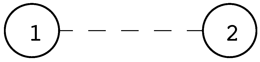
Example: Every 0-complex is a 0-maniplex, isomorphic to this one: $\mathrm{\Omega }=\{1,2\},r_0=\left\{\{1,2\}\right\}.$

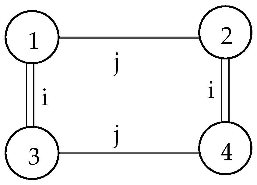
Example: Every 1-complex is a 1-maniplex, and can be regarded geometrically as a polygon or 2-polytope. $\mathrm{\Omega }=\{1,2,3,4,5,6,7,8\}$, $r_0=\{\{1,2\},\{3,4\},\{5,6\},\{7,8\}\}$, $r_1=\{\{2,3\},\{4,5\},\{6,7\},\{8,1\}\}$. This maniplex has four vertices ($\{2,3\},\{4,5\}$, etc.), and four edges ($\{1,2\},\{3,4\},\cdots$); thus it is a 4-gon.

Figure 3. A 1-maniplex.

Figure 3. A 1-maniplex.

Example: A 2-maniplex. The 2-maniplex shown in Figure 4 has four faces (the 0–1 cycles), four vertices (the 1–2 cycles) and 6 edges (the 0–2 cycles). Each vertex shares an edge with each other vertex and so has degree 3. Similarly each face has three sides and so this maniplex is the tetrahedron.

One of the consequences of the definition is that if $i>j+1$, then within the i-maniplex $[r_0,r_1,\cdots ,r_i]$, two flags (1 and 2 in Figure 5) which are j-adjacent are in the same subfacet. Since $r_i$ is an isomorphism of subfacets, these must be i-adjacent to two flags which are j-adjacent, as in Figure 5.

Thus, whenever i and j differ by more than 1, then $r_i$ and $r_j$ must commute. Any group defined by having generators $[r_0,r_1,\cdots ,r_n]$ and relations which require that $|i-j|>1$ implies that $r_i$ and $r_j$ commute, is called a Coxeter string group. Thus, a maniplex is essentially a transitive action of a Coxeter string group. Conversely, any transitive action of a Coxeter string group on a set is a maniplex (as long as no generator has a fixed point). We could, in fact, use that as the definition of a maniplex.

Let $\mathrm{\Lambda }$ be the vertex set of any one component of the distance-2 graph of $\mathrm{\Gamma }$. To say that another way, $\mathrm{\Lambda }$ is the orbit of some flag under the group $C^{+}\left(\mathcal{M}\right)$ generated by all products of the form $r_i{r}_j$. If $\mathrm{\Lambda }=\mathrm{\Omega }$, we will call the maniplex non-orientable, and we call it orientable if otherwise. More briefly, $\mathcal{M}=(\mathrm{\Omega },\mathcal{A})$ is orientable if and only if $\mathrm{\Gamma }$ is bipartite.

Fact: Every map can be considered as a 2-maniplex.

Moreover, the converse is true as well: Every finite 2-maniplex has an embodiment as a map. We see this by the following construction: Given a finite 2-maniplex $\mathcal{M}=(\mathrm{\Omega },[r_0,r_1,r_2])$, assemble a set of right triangles in which each one has one leg darkened. Label each triangle with an element of $\mathrm{\Omega }$. For each $x\in \mathrm{\Omega }$, identify the light leg of triangle x with the light leg of triangle $x{r}_0$, the dark leg of triangle x with the dark leg of triangle $x{r}_2$, and the hypotenuse of x with the hypotenuse of $x{r}_1$. (Yes, yes, we must be more careful than that: In the $r_0$ and $r_2$ attachments, the right angles must meet and in the $r_1$ attachment, the two darkened legs must adjoin.) The result is a surface, and the darkened edges form a graph on the surface. The complement of the graph in the surface has components which are connected by $r_0$ and $r_1$, and hence each forms a disc. A similar construction shows that an infinite 2-maniplex in which $r_0{r}_1$ and $r_1{r}_2$ are of finite orders has an embodiment as a tessellation of some non-compact surface.

Thus maniplexes generalize maps to higher dimensions.

On the other hand, the flag graph of any abstract $(n+1)$-polytope satisfies the requirements for an n-maniplex, and so maniplexes generalize polytopes as well. Notice, incidentally, the disparity in dimension in these two notations. The word “cube", for example, can refer to the three-dimensional solid or to its 2-dimensional surface. It is thus a 3-polytope and a 2-maniplex.

6. Non-Polytopal Maps

It is important to note that abstract polytopes do not themselves generalize maps. To show that they do not, we will present two examples of maps, and hence maniplexes, which are not polytopes.

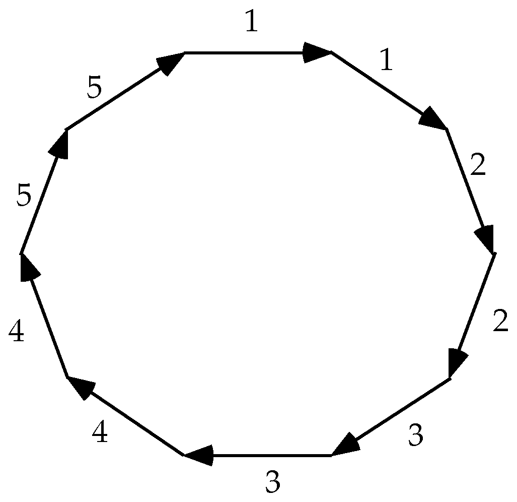
First, consider the map shown in Figure 6.

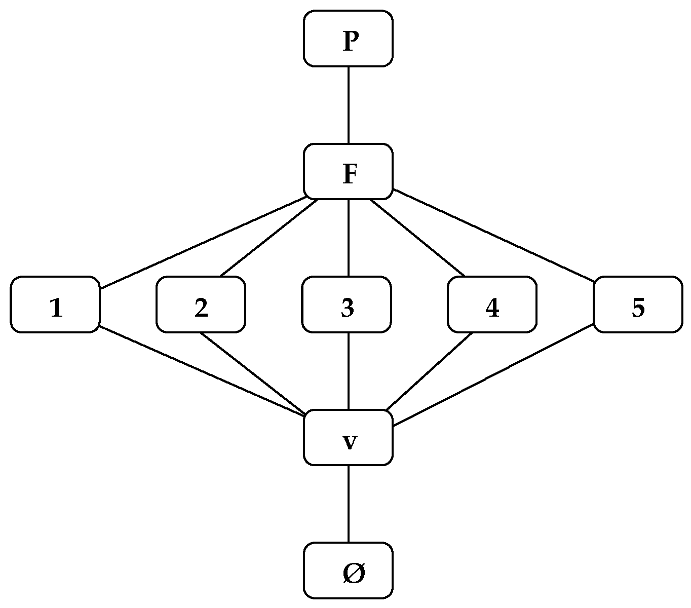
By examining the identifications making the map, one can see that it has the one face F, the five edges 1, 2, 3, 4, 5 and just one vertex v. That says that the poset of faces is as in Figure 7.

We see that the poset is not sufficiently detailed to capture the structure of the map. For instance, we cannot, from the poset, determine which edges are consecutive around F. This map also fails the diamond condition, as F and v have more than two edges in common.

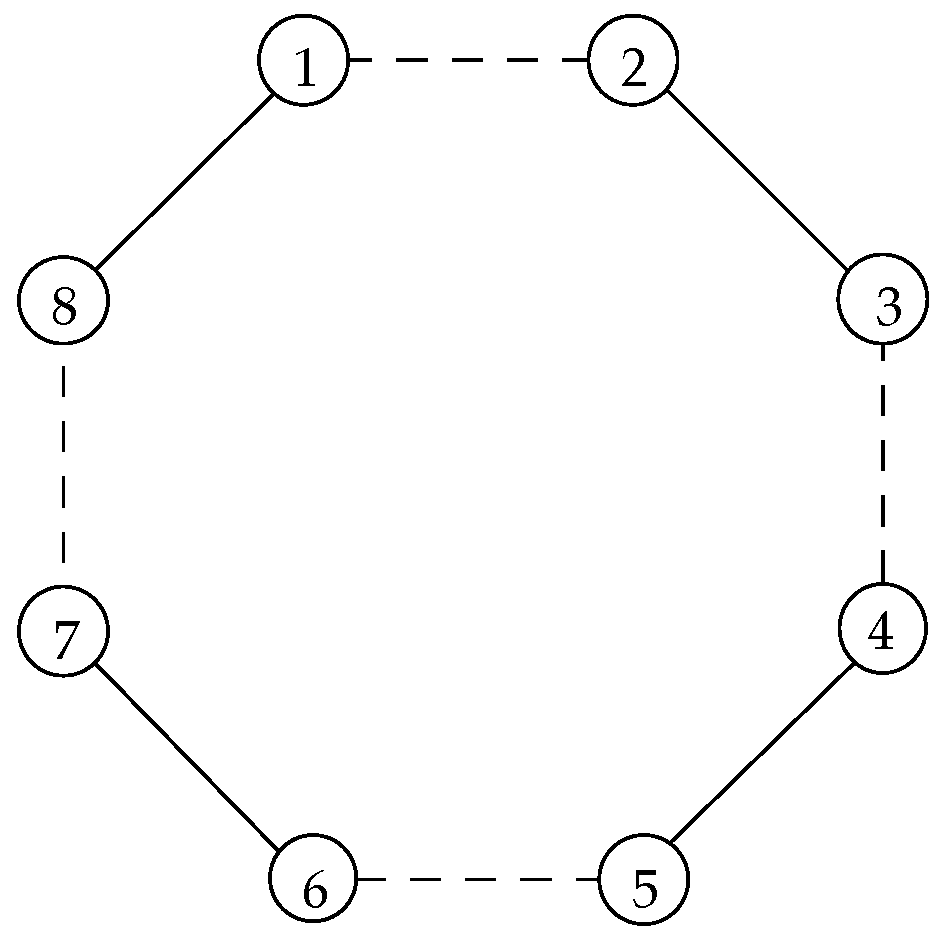
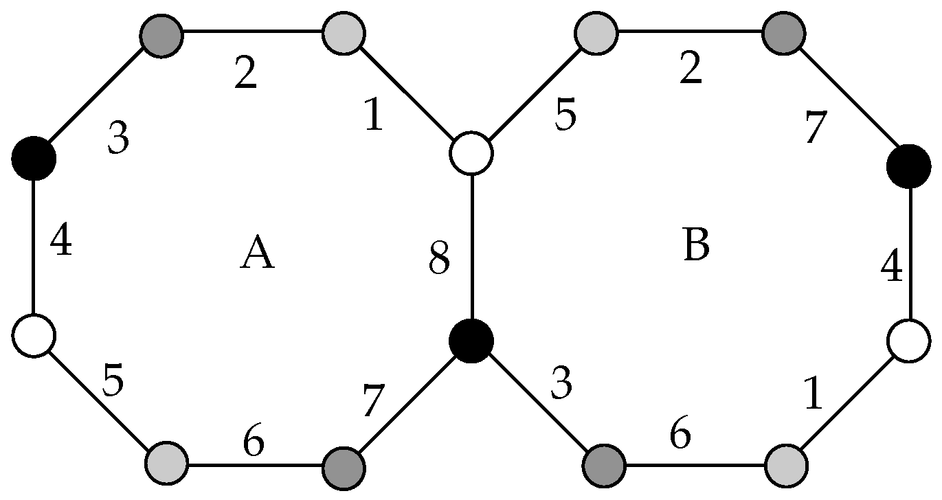
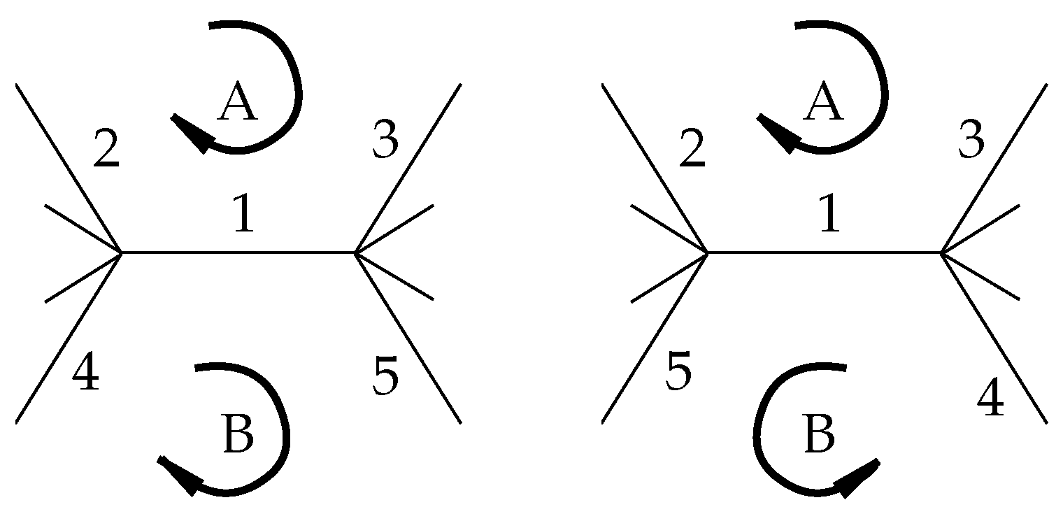
Figure 8 shows an orientable map made of two octagons, A and B, with sides identified as indicated by the edge numbers and the colors of the vertices. If we follow the identifications, we see that there are exactly 4 vertices, each of degree 4.

This map is small, but very interesting for its size. It has many symmetries and is in fact a reflexible map (defined in the next section). It is thus something that we would like to include in our study. However, the map does not qualify as an abstract polytope, as the diamond condition fails: Face A and the white vertex share not only edges 1 and 8 but also 4 and 5. Thus it is a non-polytopal map. This is not at all uncommon among maps.

7. Symmetry in Maniplexes

A symmetry or automorphism of the maniplex $\mathcal{M}=(\mathrm{\Omega },\mathcal{A})$ is an isomorphism of $\mathcal{M}$ onto itself. It is thus a color-preserving symmetry of the graph $\mathrm{\Gamma }$. Therefore, $\sigma \in S_{\mathrm{\Omega }}$ is a symmetry of $\mathcal{M}$ if and only if $\sigma$ commutes with each of the permutations $r_i$ (and thus with all of the connection group). The symmetries form a group, $Aut\left(\mathcal{M}\right)$. Recall that $\mathrm{\Lambda }$ is an orbit under the group $C^{+}\left(\mathcal{M}\right)$, which is generated by all words in the $r_i$’s of length 2. Define $Au{t}^{+}\left(\mathcal{M}\right)$ to be the subgroup of $Aut\left(\mathcal{M}\right)$ which sends $\mathrm{\Lambda }$ to itself. We will say that $\mathcal{M}$ is rotary provided that $Au{t}^{+}\left(\mathcal{M}\right)$ is transitive on $\mathrm{\Lambda }$ and reflexible provided that $Aut\left(\mathcal{M}\right)$ is transitive on $\mathrm{\Omega }$. Clearly, any non-orientable rotary maniplex is reflexible. Within the domain of rotary maniplexes, chiral means not reflexible.

The word “regular” has been used to describe maps and polytopes with large symmetry groups. Unfortunately, the word has meant different things in the two topics. Map theorists, beginning, perhaps, with Brahana, use “regular” to describe maps with rotational symmetries, i.e., rotary maps. Polytope theorists have used “regular” to mean flag-transitive, i.e., reflexible. The compromise language of maniplexes is intended to use words that mean what they say.

If $\mathcal{M}$ is any rotary n-maniplex, then for $0<i\le n$, the subgraph of $\mathrm{\Gamma }$ consisting of edges in $r_{i-1}\cup r_i$ will be a collection of disjoint cycles. If $\mathcal{M}$ is rotary, these cycles will be of the same length, $2p_i$. Then the n-tuple $\{p_1,p_2,p_3,\cdots ,p_n\}$ is the Schläfli symbol or, more briefly, the type of $\mathcal{M}$. For example, the dodecahedron is of type $\{5,3\}$, the n-dimensional cube has type $\{4,3,3,\cdots ,3\}$, and the 600-cell is of type $\{3,3,5\}$.

If $\mathcal{M}=(\mathrm{\Omega },[r_0,r_1,\cdots ,r_n])$ is a reflexible n-maniplex and I is any one fixed flag, then for each i, there is a unique symmetry ${\alpha }_i$ taking I to $I{r}_i$. Because symmetries commute with the connection group, we have that for all i and j, $I{\alpha }_i{\alpha }_j=I{r}_i{\alpha }_j=I{\alpha }_j{r}_i=I{r}_j{r}_i$. This implies that the correspondence ${\alpha }_i\leftrightarrow r_i$ extends to an antimorphism between $Aut\left(\mathcal{M}\right)$ and $C\left(\mathcal{M}\right)$. Thus, for a reflexible maniplex, the connection group and the symmetry group are isomorphic. For more on symmetry in maps see [15,16].

8. Operators on maniplexes

In maps, we often find it illuminating to consider relations between two maps. It is useful to describe operators, constructions which, given one map, make another, related map. The paper [17] considers many such operators in detail, as does [18]. We wish to generalize these to maniplexes; fortunately, this is straightforward:

If $\mathcal{M}=(\mathrm{\Omega },\mathcal{A})$, and $\mathcal{A}=[r_0,r_1,\cdots ,r_n]$, the dual of $\mathcal{M}$, denoted $D\left(\mathcal{M}\right)$, has the same flag set $\mathrm{\Omega }$, but the reversed sequence ${\mathcal{A}}^{\prime }=[r_n,r_{n-1},\cdots ,r_1,r_0]$. It is not obvious from the recursive definition that this is a maniplex, but the alternative definition as an action of a Coxeter string group with fixed-point free generators makes that clear.

We define the Petrie of $\mathcal{M},P\left(\mathcal{M}\right)$, to have sequence ${\mathcal{A}}^{\prime }$ identical to $\mathcal{A}$ except at the entry of index $n-2$: $[r_0,r_1,\cdots ,r_{n-3},r_{n-2}^{\prime }=r_n{r}_{n-2},r_{n-1},r_n]$. In order for this to qualify as a maniplex, $r_{n-2}^{\prime }$ must be an involution and commute with all other generators except, possibly, $r_{n-3}$ and $r_{n-1}$. Clearly, $r_{n-2}^{\prime }$ is an involution because $r_n$ and $r_{n-2}$ commute with each other. It commutes with $r_n$ because $r_{n-2}$ does. And it commutes with all $r_i$ for $i\le n-4$ because they commute with $r_n$ and $r_{n-2}$.

Similarly, we define the opposite of $\mathcal{M}$, denoted $opp\left(\mathcal{M}\right)$, to have sequence $[r_0,r_1,r_2^{\prime }=r_0{r}_2,r_3,\cdots ,r_n]$.

Now, $opp$ has an interesting effect on maps: if $\mathcal{M}$ is a map, then $opp\left(\mathcal{M}\right)$ has the same faces but at each edge, the meeting of the faces is reversed, as in Figure 9.

For example, if $\mathcal{M}$ is the tetrahedron, then $opp\left(\mathcal{M}\right)$ is the hemi-octahedron of type $\{3,4\}$ on the projective plane.

The effect of $opp$ on higher-dimensional maniplexes is interesting and clear: if the facets of $\mathcal{M}$ are copies of the $(n-1)$-maniplex $\mathcal{F}$ for $n>2$, then the facets of $opp\left(\mathcal{M}\right)$ are copies of the $(n-1)$-maniplex $opp\left(\mathcal{F}\right)$, and the $r_n$ connections are the same in both maniplexes. Because the change between $\mathcal{M}$ and $opp\left(\mathcal{M}\right)$ happens at the $i=2$ level only, all $i-$faces in $opp\left(\mathcal{M}\right)$ for $i>2$ are $opp$ of their counterparts in $\mathcal{M}$.

The general effect of the Petrie operator is less easy to visualize; our best hope here is to realize that $P=D$ $opp$ D. The maniplexes related to $\mathcal{M}$ via $D,P,opp$ and their products are the direct derivates of $\mathcal{M}$. We note that the class of maniplexes is closed under these operations.

If $n=2$, so that the maniplex is a map, $opp$ is also equal to $PDP$, and so $\mathcal{M}$ has at most 6 direct derivates. For any higher value of n, we have $Popp=oppP$, and so we get at most 8 direct derivates from one maniplex. Thus the operators act as $D_3$ or $D_4$ on the direct derivates of each map.

Even in seemingly simple cases these operators can produce surprising results. For example, let $\mathcal{M}=$ the 4-simplex. This is a 4-polytope, a 3-maniplex, of type $\{3,3,3\}$. It consists of 5 tetrahedra, assembled so that three facets surround each edge. It has 5 facets, 10 triangular faces, 10 edges and 5 vertices, and is isomorphic to its dual.

For this maniplex, $P\left(\mathcal{M}\right)$ is a 3-maniplex of type $\{6,4,3\}$; it has the same 5 vertices, and the same 10 edges. It has 10 hexagonal 2-faces, and, shockingly, just one facet. The facet is isomorphic to the map $\mathcal{N}={\{6,4|3\}}_5$. This map has 10 hexagonal faces; these are the subfacets of the maniplex. The map has 30 edges and 15 vertices. It is formed from Coxeter’s regular skew polyhedron $\{6,4|3\}$ by identifying vertices, edges, faces which are antipodal in some Petrie path. The connector $r_3$ joins each flag of $\mathcal{N}$ to the one diametrically opposite to it in its face. This surprising non-polytopal maniplex would not have been found without the use of the operator P.

We also define a “bubble” operator $B_j$, analogous to the “hole” operator, $H_j$, defined for maps. The effect of this on $\mathcal{M}$ is to replace $r_{n-1}$ with $r_{n-1}{\left(r_n{r}_{n-1}\right)}^{j-1}$. As in the map case, the result might not be connected and so we define $B_j\left(\mathcal{M}\right)$ to be any one component of the result.

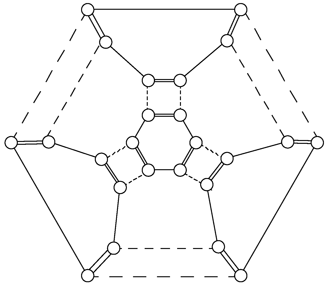
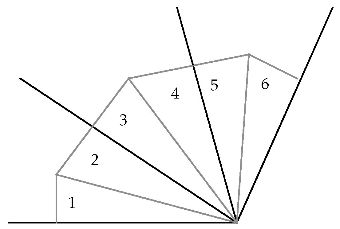
To visualize the effect of the operator $B_j$, it may help to consider Figure 10, which shows a simplified view of facets and subfacets arranged about a subsubfacet.

In this figure, the solid lines represent subfacets, the common point of these lines is the subsubfacet, and the wedges of space between the solid lines represent facets. Then triangle 1 represents a typical flag f, triangle 2 is $f{r}_{n-1}$, and 3 is $f{r}_{n-1}{r}_n$. Similarly, 4 and 6 are $f{r}_{n-1}{\left(r_n{r}_{n-1}\right)}^1$ and $f{r}_{n-1}{\left(r_n{r}_{n-1}\right)}^2$. Thus the connector $r_{n-1}{\left(r_n{r}_{n-1}\right)}^{j-1}$ links each subfacet to those which are separated from it by j facets. These subfacets join by the new $(n-1)$-connector to form “bubbles” which are the facets of the new maniplex.

For instance, in the 600-cell, which is composed of 600 regular tetrahedra arranged so that 5 of them surround every edge, each vertex v is incident with 20 tetrahedral facets. The 20 triangles opposite to v in this configuration form an icosahedron. Thus $B_2$ of the 600-cell is a maniplex whose facets are icosahedra, meeting 5 at each edge. In the geometric 600-cell, $B_2$ produces the star-polytope called the icosahedral 120-cell.

The maniplexes related to $\mathcal{M}$ through all products of $D,P,opp,B_j$ are the derivates of $\mathcal{M}$.

The derivates of a maniplex give a potentially very large class of maniplexes which are related to each other. Understanding any one of them, then, will increase our understanding of the others.

9. Conclusions

There are many interesting open questions regarding maniplexes. Here are just a few of them:

(1)

Can we classify all rotary maniplexes having one facet? Two facets? In maps, the classifications of 1-face and 2-face maps are easy and all such maps are reflexible. In maniplexes, several examples of chiral 1-facet and 2-facet 3-maniplexes are known.

(2)

What conditions on a polytope will guarantee that all of its derivates are polytopal as well?

(3)

Given a rotary map $\mathcal{M}$, what are all the rotary 3-maniplexes having facets isomorphic to $\mathcal{M}$?

(4)

Given a graph $\mathrm{\Gamma }$, what are all the rotary maniplexes whose 1-skeleton is isomorphic to $\mathrm{\Gamma }$?

References

- Miklivič, S.; Potpčnik, P.; Wilson, S. Consistent cycles in graphs and digraphs. Graphs Combin. 2007, 23, 205–216. [Google Scholar] [CrossRef]
- Miklivič, S.; Potočnik, P.; Wilson, S. Overlap in consistent cycles. J. Graph Theory 2007, 55, 55–71. [Google Scholar] [CrossRef]
- Monson, B.; Schulte, E.; Pisanski, T.; Weiss, A.I. Semisymetric graphs from polytopes. J. Comb. Theory A 2007, 114, 421–435. [Google Scholar] [CrossRef]
- Monson, B.; Weiss, A.I. Medial Layer Graphs of Equivelar 4-polytopes. Eur. J. Combin. 2007, 28, 43–60. [Google Scholar] [CrossRef]
- Conder, M.; Hubard, I.; Pisanski, T. Constructions for chiral polytopes. J. London Math. Soc. 2008, 77, 115–129. [Google Scholar] [CrossRef]
- Coxeter, H.S.M. The Edges and faces of a 4-dimensional polytope. Congres. Numerantium 1980, 28, 309–334. [Google Scholar]
- Hubard, I. Two-orbit polyhedra from groups. Eur. J. Combin. 2010, 31, 943–960. [Google Scholar] [CrossRef]
- Hubard, I.; Orbanič, A.; Weiss, A.I. Monodromy groups and self-invariance. Can. J. Math. 2009, 61, 1300–1324. [Google Scholar] [CrossRef]
- Hubard, I.; Weiss, A.I. Self-duality of chiral polytopes. J. Comb. Theory A 2005, 111, 128–136. [Google Scholar] [CrossRef]
- McMullen, P.; Schulte, E. Abstract Regular Polytopes, 1st ed.; Cambridge University Press: Cambridge, UK, 2002. [Google Scholar]
- Pellicer, D.A. Construction of higher rank polytopes. Discret. Math. 2010, 310, 1222–1237. [Google Scholar] [CrossRef]
- Schulte, E. Regulàre Inzidenzkomplexe, Universitát DortmE. und Dissertation. 1980.
- Schulte, E. Symmetry of polytopes and polyhedra. In Handbook of Discrete and Computational Geometry, 2nd ed.; Goodman, J.E., O’Rourke, J., Eds.; CRC Press: Boca Raton, FL, USA, 2004. [Google Scholar]
- Vince, A. Combinatorial maps. J. Comb. Theory B 1983, 34, 1–21. [Google Scholar] [CrossRef]
- Coxeter, H.S.M.; Moser, W.O.J. Generators and Relations for Discrete Groups, 4th ed.; Springer-Verlag: New York, NY, USA, 1980. [Google Scholar]
- Orbanič, A.; Pellicer, D.; Tucker, T. Edge-transitive Maps of Low Genus. Ars Math. Cont. 2011, 4, 385–402. [Google Scholar] [CrossRef]
- Wilson, S. Operators over regular maps. Pacific J. Math. 1979, 81, 559–568. [Google Scholar] [CrossRef]
- Orbanič, A.; Pellicer, D.; Weiss, A.I. Map Operations and K-orbit Maps. J. Comb. Theory A 2010, 117, 411–429. [Google Scholar] [CrossRef]
Figure 1.
Flags in a map.
Figure 2.
A 0-maniplex.
Figure 4.
The tetrahedron as a 2-maniplex.
Figure 5.
Within an i-face.
Figure 6.
A map with one face.
Figure 7.
The poset of the map.
Figure 8.
Faces and vertices in the map .
Figure 9.
An edge in a map and its opposite.
Figure 10.
Facets and subfacets.
© 2012 by the author; licensee MDPI, Basel, Switzerland. This article is an open access article distributed under the terms and conditions of the Creative Commons Attribution license (http://creativecommons.org/licenses/by/3.0/).
Share and Cite
MDPI and ACS Style
Wilson, S. Maniplexes: Part 1: Maps, Polytopes, Symmetry and Operators. Symmetry 2012, 4, 265-275. https://doi.org/10.3390/sym4020265
AMA Style
Wilson S. Maniplexes: Part 1: Maps, Polytopes, Symmetry and Operators. Symmetry. 2012; 4(2):265-275. https://doi.org/10.3390/sym4020265
Chicago/Turabian StyleWilson, Steve. 2012. "Maniplexes: Part 1: Maps, Polytopes, Symmetry and Operators" Symmetry 4, no. 2: 265-275. https://doi.org/10.3390/sym4020265