Hexagonal Inflation Tilings and Planar Monotiles

1
Fakultät für Mathematik, Universität Bielefeld, Postfach 100131, Bielefeld 33501, Germany
2
Department of Mathematics and Statistics, The Open University, Walton Hall, Milton Keynes MK7 6AA, UK
*
Author to whom correspondence should be addressed.
Symmetry 2012, 4(4), 581-602; https://doi.org/10.3390/sym4040581
Submission received: 2 September 2012
/
Revised: 8 October 2012
/
Accepted: 14 October 2012
/
Published: 22 October 2012
(This article belongs to the Special Issue Polyhedra)
Abstract
:Aperiodic tilings with a small number of prototiles are of particular interest, both theoretically and for applications in crystallography. In this direction, many people have tried to construct aperiodic tilings that are built from a single prototile with nearest neighbour matching rules, which is then called a monotile. One strand of the search for a planar monotile has focused on hexagonal analogues of Wang tiles. This led to two inflation tilings with interesting structural details. Both possess aperiodic local rules that define hulls with a model set structure. We review them in comparison, and clarify their relation with the classic half-hex tiling. In particular, we formulate various known results in a more comparative way, and augment them with some new results on the geometry and the topology of the underlying tiling spaces.
1. Introduction
A well-known inflation rule with integer inflation factor is the half-hex inflation from [1], Exercise 10.1.3 and Figure 10.1.7, which we show in Figure 1. As such, it is a lattice substitution (or inflation) in the sense of [2,3]. Moreover, it is a face to face stone inflation (in the sense of Danzer), which means that each inflated tile is precisely dissected into copies of the prototile so that the final tiling is face to face. This rule defines an aperiodic tiling of the plane, but it does not originate from an aperiodic prototile set (for the terminology, we refer to [4] and references therein). In principle, the procedure of [5] can be applied to add local information to the prototile and to the inflation rule (via suitable markers and colours), until one arrives at a version with an aperiodic prototile set. However, to our knowledge, this has never been carried out, as it (most likely) would result in a rather large prototile set.
Figure 1.
Half-hex inflation rule.
Interestingly, two different inflation rules for hexagonally shaped prototiles have independently been constructed, namely one by Roger Penrose [6] and one by Joan Taylor [7] (see also [8]), each defining a tiling hull that can also be characterised by aperiodic local rules. Viewed as dynamical systems under the translation action of , they both possess the continuous half-hex hull (and also the arrowed half-hex, to be introduced later) as a topological factor, though with subtle differences. They may be considered as covers of the half-hex that comprise just enough local information to admit an aperiodic prototile set. In fact, both examples are again lattice inflations. They were found in the attempt to construct an aperiodic planar monotile, which loosely speaking is a single prototile together with some local rules that tiles the plane, but only non-periodically. Let us mention that Taylor’s original inflation tiling can be embedded into a slightly larger tiling space that still possesses aperiodic local rules [8], but is no longer minimal (see below for more on minimality).
All three, the half-hex, the Penrose and the Taylor tiling, are structures that can be described as model sets; see [9,10,11] for background on model sets. For the half-hex tiling, this was first shown in [12]. Observing that two half-hexes always join to form a regular hexagon, with edge length 1 say, one obtains a hexagonal packing where three types of hexagons are distinguished by a single diagonal line. We represent each hexagon by a single point located at its centre, of type , where ℓ corresponds to a diagonal that is rotated by against the horizontal. This gives a partition
with , where Γ is a triangular lattice of density . When starting from a fixed point tiling of the half-hex inflation rule, the fixed point equations for the three point sets lead to the solution
where the are empty sets except for one, which is the singleton set . Where the latter occurs depends on the seed of the selected fixed point. This means that there are precisely three possibilities, corresponding to the three possible choices for the central hexagon; see [9] for the detailed derivation.
This description establishes the model set structure, with the 2-adic completion of Γ as internal space. Note that the point 0 is the unique limit point of any of the three unions in Equation (1) in the 2-adic topology. The structure of the union over expanded and shifted copies of Γ is also called a Toeplitz structure. It is an example of a limit-periodic system [13] with pure point diffraction (and, equivalently, with pure point dynamical spectrum [14,15,16]). The diffraction measure of a weighted Dirac comb on the half-hex tiling can be calculated from Equation (1) via the Poisson summation formula, by an application of the methods explained in [9,17]. This description of the half-hex tiling will be the key observation to also identify the two covers (by Penrose and by Taylor) as model sets.
Below, we discuss the two inflation tilings due to Penrose and Taylor in some detail. To be more precise with the latter case, we only consider the minimal part of the tiling space considered by Socolar and Taylor in [8]. This minimal part is the tiling LI (local indistinguishability) class defined by Taylor’s original stone inflation rule [7]. To distinguish the two hulls, we use the term Taylor tiling for the minimal inflation hull and refer to the elements of the larger tiling space as the Socolar–Taylor tilings.
We assume the reader to be familiar with the concept of mutual local derivability (MLD), which was introduced in [18]; see also [9,19]. When the derivation rules commute with all symmetries of the tilings under consideration (respectively their hulls), they are called symmetry preserving. The corresponding equivalence classes are called SMLD classes [19].
The hull of a (planar) tiling with finite local complexity (FLC) in is defined as the orbit closure in the local topology, . Here, two tilings are ε-close when they agree on the ball , possibly after (globally) translating one of them by an element from . Due to the FLC property, the hull is compact [16], with continuous action of the group via translation. Consequently, the pair is a topological dynamical system. It is called minimal when the translation orbit of every element of the hull is dense in it. Our examples below will be minimal hulls of FLC tilings, or of equivalent representatives of the corresponding MLD class.
A hull is called aperiodic when no element of it possesses non-trivial periods. In other words, is aperiodic when, for every , the equation only holds for . A hull is said to have local rules when it is specified by a finite list of legal local configurations, for instance in the form of a finite atlas of patches. If a set of local rules specifies an aperiodic hull, the rules themselves are called aperiodic. When a set of rules specifies a hull that is minimal, they are called perfect. Of special interest now are local rules that are aperiodic and perfect, such as the well-known arrow matching conditions of the classic rhombic Penrose tiling; compare [1].
A single prototile, assumed compact and simply connected, is called a monotile (in the strict sense) when a set of aperiodic perfect local rules exists that can be realised by nearest neighbour matchings only. A subtle question in this context is whether one allows reflected copies of the prototile or not. Quite often, geometric matching conditions are replaced by suitable decorations of the prototile together with rules how these decorations have to form local patterns in the tiling process. The latter need not be restricted to conditions for nearest neighbour tiles, in which case one speaks of a functional monotile to indicate the slightly more general setting. Our planar examples below are of the latter type, or even a further extension of it.
This article, which is a brief review together with some new results on the two tiling spaces, grew out of a meeting on discrete geometry that was held at the Fields Institute in autumn 2011. As such, it is primarily written for a readership with background in discrete geometry, polytopes and tilings. We also try to provide the concepts and methods for readers with a different background, though this is often only possible by suitable pointers to the existing literature. In particular, where correct and complete proofs are available, we either refer to the original source or sketch how the arguments have to be applied to suit our formulation. As is often the case in discrete geometry, following a proof might need some pencil and paper activity on the side of the reader; compare the introduction and the type of presentation in [1]. This is particularly true of arguments around local derivation rules, inflation properties and aperiodic prototile sets.
When we prepared this manuscript, we rewrote known results on both tiling spaces in a way that emphasises their similarities, and mildly extended them, for instance by the percolation property of two derived parity patterns. Moreover, we calculated several topological invariants of the tiling spaces under consideration, which (as far as we are aware) were not known before. In order not to create an imbalance, we only describe how to do that in principle (again with proper references) and then state the results. We also include the dynamical zeta functions for the inflation action on the hulls, which are the generating functions for the corresponding fixed point counts. They turn out to be particularly useful for deriving the structure of the hull. Since several examples of a similar nature have recently been investigated in full detail, compare [20,21,22], we felt that this short account is adequate (in particular, as the explicit results are the outcome of a computer algebra program).
The paper is organised as follows. In Section 2, we begin with a discussion of the -tiling due to Penrose, together with various other elements of the MLD class defined by it. Section 3 contains the corresponding material on the Taylor (and the Socolar–Taylor) tilings and their “derivatives”, which we discuss in slightly more detail, including the percolation result on the parity patterns of both tilings. The topological invariants and various other quantities for a comparison of the tilings are presented in Section 4, which is followed by some concluding remarks and open problems.
2. Penrose’s Aperiodic Hexagon Tiling and Related Patterns
The -tiling due to Roger Penrose is built from three prototiles, up to Euclidean motions (including reflections). The tiles and the inflation rule (with linear inflation multiplier 2) are shown in Figure 2. The name -tiling refers to the three prototiles as the 1-tile (hexagon), the ε-tile (edge tile) and the -tile (corner tile). The ε-tile has a definite length, but can be made arbitrarily thin, while the -tile can be made arbitrarily small. This inflation rule is not primitive, but still defines a unique tiling LI class in the plane via a fixed point tiling with a hexagon at its centre. A patch of such a tiling is shown in Figure 3. There are 12 fixed point tilings of this type, each defining the same LI class. These fixed points form a single orbit under the symmetry of the LI class.
The following result was shown in [6] by the composition-decomposition method; see [23] for a detailed description of this method.
Proposition 1
The inflation rule of Figure 2 defines a unique tiling LI class with perfect aperiodic local rules. The latter are formulated via an aperiodic prototile set, which consists of the three tiles from Figure 2 (together with rotated and reflected copies). The rules are then realised as purely geometric matching conditions of the tiles. ☐
Figure 2.
Inflation rule for Penrose’s -tiling.

Figure 3.
Patch of Penrose’s -tiling.

In the original publication [6], it was argued that this system comes “close” to an aperiodic monotile in the sense that it is essentially a marked hexagon tiling with matching conditions that are realised by “key tiles”, which can be made thin and small. A transformation to an equivalent version was only sketched briefly at the end of the article, and subsequently substantiated in [24] in the form of a puzzle and its solution. The key idea is to change from the -tiling to the double hexagon tiling of Figure 4, which is possible by the local derivation rule sketched in Figure 5, when read from left to right.
Figure 4.
A patch of the double hexagon tiling, exactly corresponding to that of Figure 3.
Figure 4.
A patch of the double hexagon tiling, exactly corresponding to that of Figure 3.
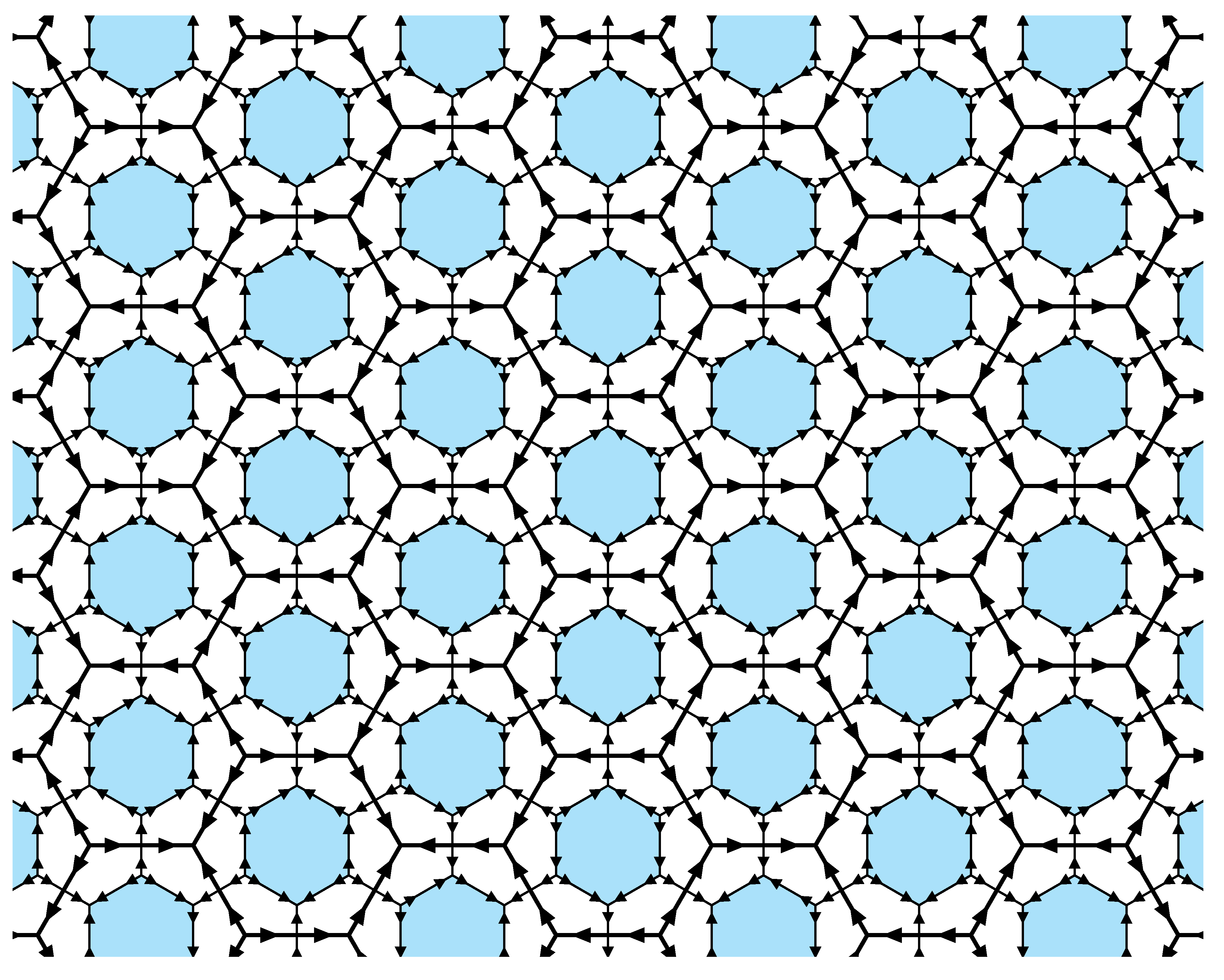
Figure 5.
Rules for the mutual local derivation between -tilings and double hexagon tilings.
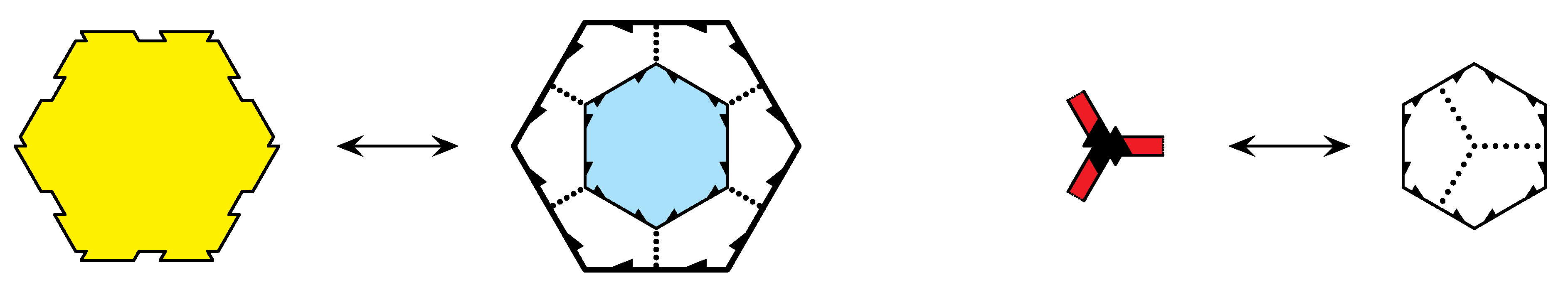
The actual rule consists of two steps. In the first, each hexagonal 1-tile is replaced by a double hexagon as shown in the left panel of Figure 5. This produces a complete tiling of the larger hexagons (with matching arrows) with fully oriented inscribed hexagons, while all remaining small hexagons, namely those around the vertices of the larger hexagons, are still incomplete (thin dotted lines). Their missing orientations derive consistently from the -tiles via the rule shown in the right panel.
Note that all hexagons (which means on both scales) have the same type of arrow pattern. In particular, each hexagon has precisely one pair of parallel edges that are oriented in the same direction, while all other arrows point towards the two remaining (antipodal) vertices. Note that this is the same edge orientation pattern as seen at the boundary of the hexagonal 1-tile in Figure 2 and Figure 3.
The derivation rule specified in Figure 5 is clearly local in both directions, and commutes with the translation action as well as with all symmetry operations of the group (the symmetry group of the regular hexagon). The following result is thus obvious.
Proposition 2
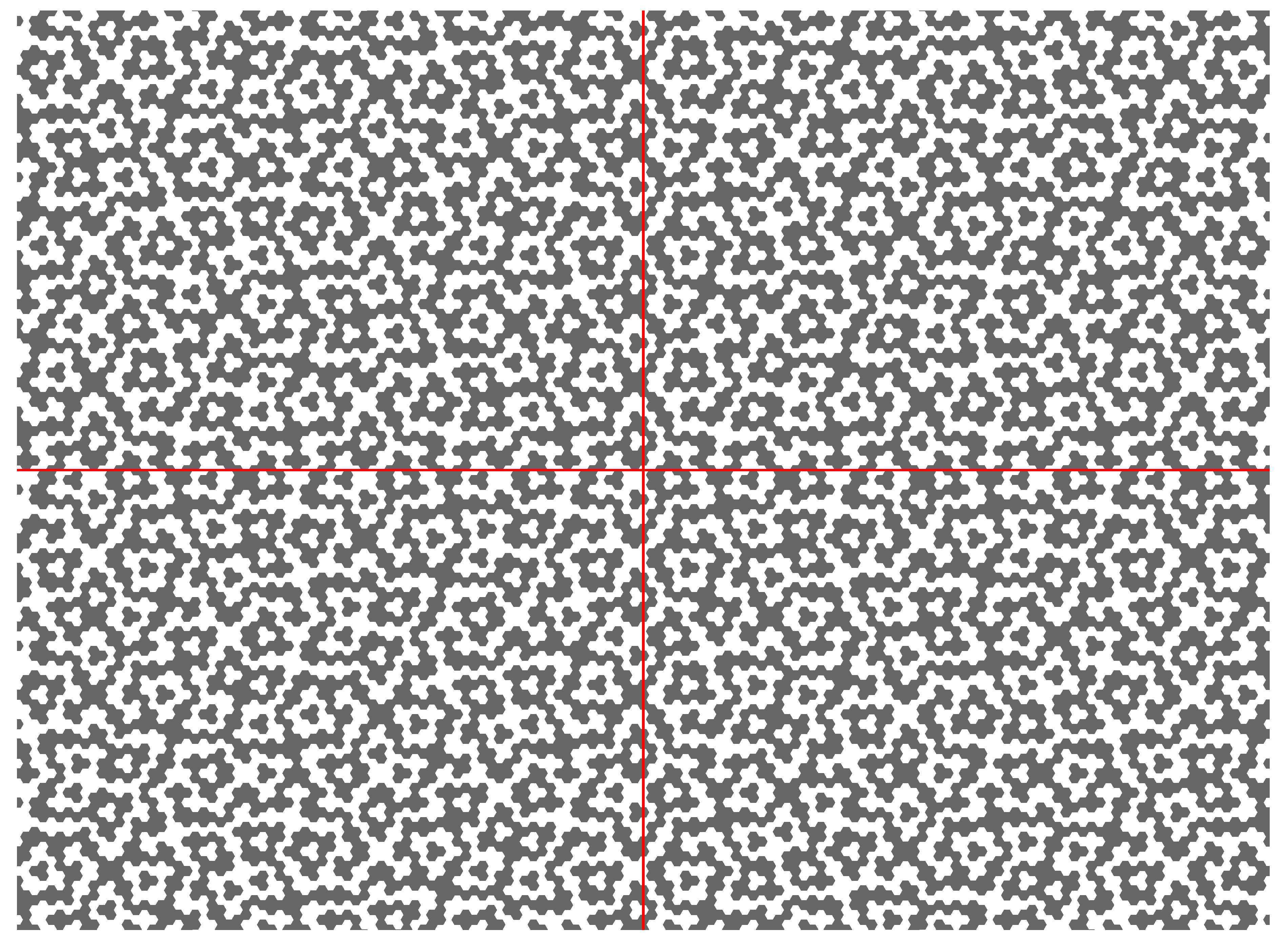
A closer inspection of the prototile set of Figure 2 reveals that the hexagonal 1-tile occurs in two chiralities with six orientations each. Keeping track of the chiralities only (by two colours, white and grey say) and disregarding all other structural elements provides a local derivation from the -tiling to an ensemble of 2-colourings of the hexagonal packing. An example of the latter is illustrated in Figure 6. We call the elements of this new ensemble the parity patterns of the -tilings. This parity pattern was introduced in [6], but (as far as we know) has not been further investigated. Our motive to do so will become clear from the comparison with the llama tilings in the next section. By construction, the parity patterns form a single LI class. A little surprising is the following property.
Figure 6.
Parity pattern of a -tiling, as derived from a fixed point tiling of the inflation rule of Figure 2. This particular pattern (also the infinite one) possesses an almost colour reflection symmetry with respect to the indicated lines; see text for details.
Figure 6.
Parity pattern of a -tiling, as derived from a fixed point tiling of the inflation rule of Figure 2. This particular pattern (also the infinite one) possesses an almost colour reflection symmetry with respect to the indicated lines; see text for details.

Theorem 1
Sketch of Proof.
The determination of the parity pattern that belongs to a -tiling is clearly local and preserves all symmetries, so that this direction is clear.
Conversely, starting from a parity pattern, the corresponding -tiling is locally reconstructed via hexagonal coronae of order 3. A simple computer search shows that such coronae uniquely specify the decorated hexagon that corresponds to its centre, once again in a symmetry-preserving way. ☐
Let us note that, as a result of the relation between two fixed point tilings with mirror image central hexagons, the particular parity patch of Figure 6 shows an almost reflection colour symmetry for the reflections in the two lines indicated. More precisely, under reflection and colour inversion, the patch is mapped onto itself, except for some hexagons along the reflection line.
Remark 1
The left panel of Figure 5 shows the building block of the double hexagon tiling without arrows on the dashed lines. As mentioned above, they are added by the local rule how to complete the vertex configurations. In this sense, one has a single prototile template together with a set of local rules that specify how to put them together. Any double hexagon tiling of the plane that everywhere satisfies the rules is an element of the double hexagon LI class, and in this sense one has a functional monotile template. We suggest calling this a weak functional monotile, as it stretches the monotile concept to some extent.
Let us return to the structure of the -tilings. As mentioned before, each hexagonal 1-tile possesses a unique pair of parallel edges that are oriented (by the arrows) in the same direction. If we divide it now into two half-hexes along the diagonal that is parallel to this edge pair, we can locally derive a half-hex tiling from any -tiling. An inspection of Figure 2 confirms that this derivation rule indeed induces the half-hex inflation of Figure 1. This is a local derivation of sliding block map type on the underlying hexagonal packing, hence continuous in the local topology.
Proposition 3
The LI class of the half-hex tiling as defined by the stone inflation rule of Figure 1 defines a minimal topological dynamical system under the translation action of that is a topological factor of the LI class of the -tilings defined by the inflation rule of Figure 2. The corresponding factor map is one-to-one almost everywhere, but the two tiling spaces define distinct MLD classes.
Sketch of Proof.
The first claim follows from our above description of the local derivation rule via the additional diagonal line in the hexagonal 1-tiles. The two LI classes cannot be MLD (and hence also not SMLD) because the existence of aperiodic local rules is an invariant property of an MLD class, hence shared by all LI classes that are MLD. It is well-known [1,12] that the half-hex hull has no such set of rules, because any finite atlas of patches can still be part of a periodic arrangement.
Since the -tilings have perfect aperiodic local rules by Proposition 1, the last claim is clear. The statement on the multiplicity of the mapping is a consequence of the model set structure, which we prove below in Theorem 5. ☐
The (regular) model set structure of the half-hex tiling, as spelled out in Equation (1) for the fixed points under the inflation rule, implies that there is a “torus parametrisation” map onto a compact Abelian group [16,25]. Here, it is a factor map onto the two-dimensional dyadic solenoid , which is almost everywhere one-to-one by Theorem 5 of [25]. Since the half-hex LI class is the image of the LI class under a factor map that is itself one-to-one almost everywhere (which follows by the same argument that we use below to prove Theorem 5), we know (via concatenation) that there exists an almost everywhere one-to-one factor map from the LI class onto . Then, Theorem 6 from [25] implies the following result.
Corollary 1
The LI class has a model set structure, with the same cut and project scheme as derived for the half-hex tilings. ☐
In summary, the LI class has all magical properties: It can be defined by an inflation rule, by a set of perfect aperiodic local rules, and as a regular model set. Moreover, it comes close to solving the quest for a (functional) monotile.
Let us turn our attention to a later (though completely independent) attempt of a similar kind that improves the monotile state-of-affairs.
3. Taylor’s Inflation Tiling
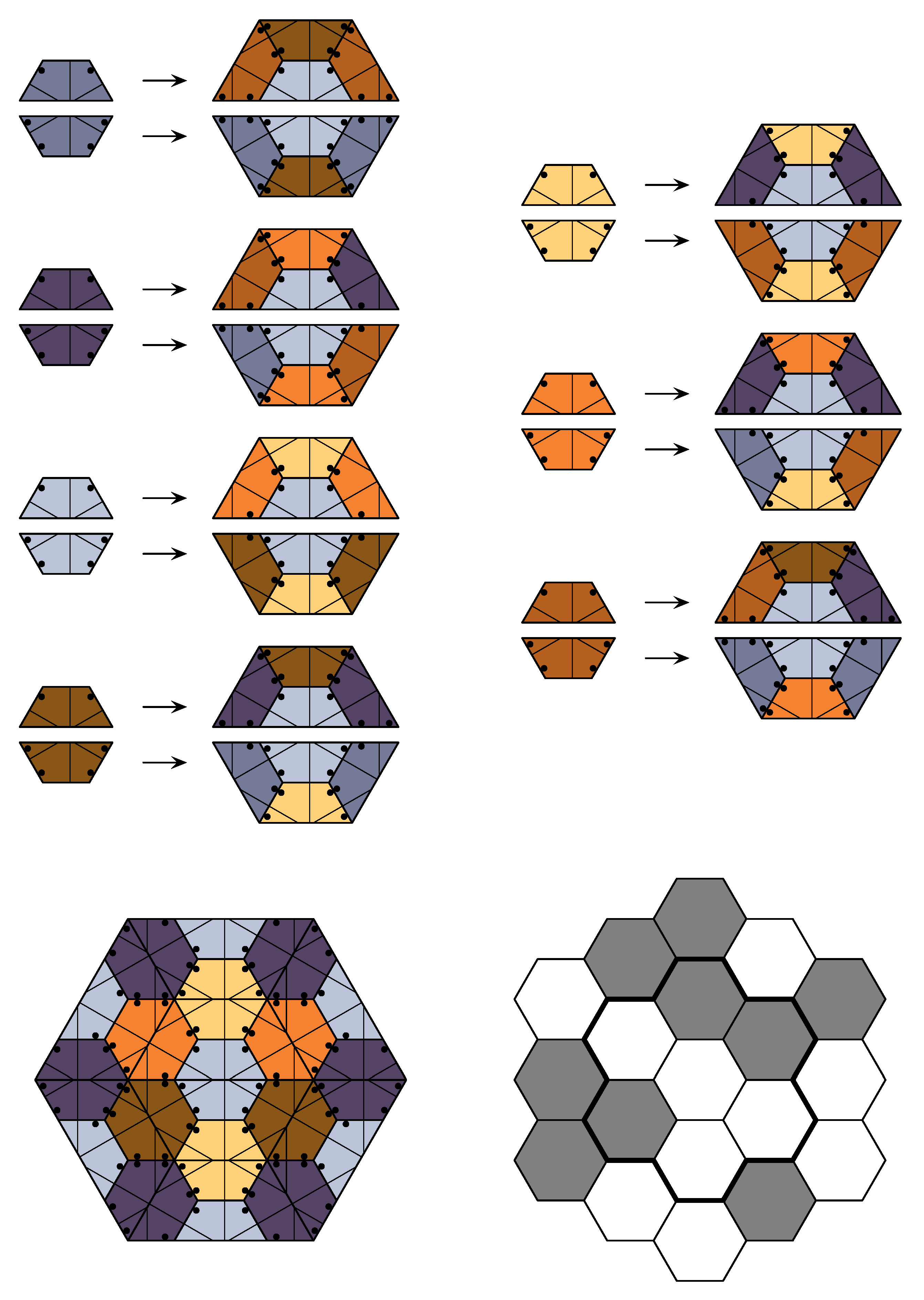
Consider the primitive stone inflation rule of Figure 7. It is formulated with 14 prototiles (up to similarity) of half-hex shape that are distinguished by colour and a decoration (with points and lines). Each half-hex occurs in two chiralities and six orientations, so that the total number of prototiles (up to translation) is 168. In the original paper [7], the 7 colours are labelled . The C-type tiles (light blue in our version) are special in the sense that they are in the centre of any fixed point tiling under the inflation rule. They are also more frequent than the other types. As mentioned above, we call the elements of the tiling space (or hull) defined by this inflation rule the Taylor tilings. The following result is immediate from Figure 7, in comparison with Figure 1, by simply removing decorations and colour.
Lemma 1
The half-hex LI class is a topological factor of the LI class of the Taylor tilings, where the latter is again minimal. In particular, the Taylor LI class is aperiodic. ☐
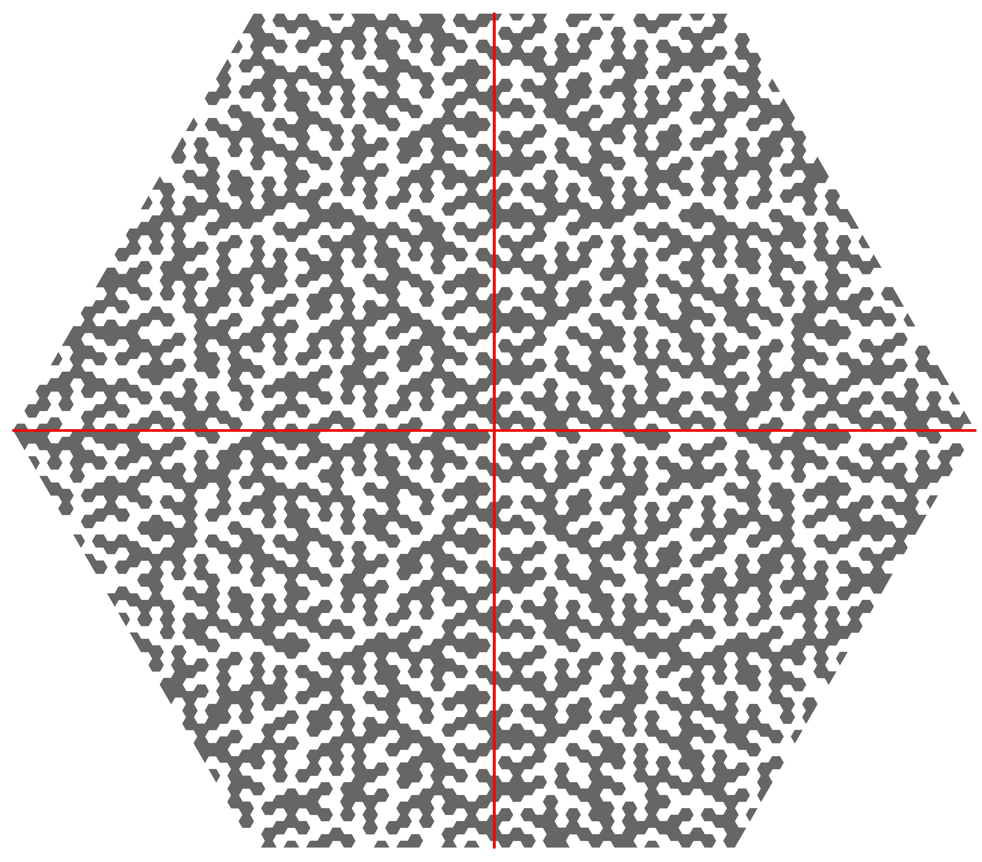
As in the case of the Penrose tiling above, one can locally derive a hexagonal parity pattern from every Taylor tiling. To this end, one considers the natural half-hex pairs, disregards their colours, and applies a grey/white coding of the two chiralities. The resulting two-coloured hexagonal packings are called llama tilings, see Figure 8 for an illustration. The name refers to the shape of the smallest island (of either colour), and was coined by Taylor. As in the previous section, the parity pattern still contains the full local information. Also, the llama tiling has the same type of almost colour reflection symmetry that we encountered in the previous section for the Penrose parity pattern.
Theorem 2
The LI class of Taylor’s inflation tiling and that of the llama tiling of Figure 8 are SMLD. In particular, the llama tiling is aperiodic.
Sketch of Proof.
As in the case of Theorem 1, the derivation of the llama tiling, which is the parity pattern of the Taylor tiling, is obviously local and symmetry preserving.
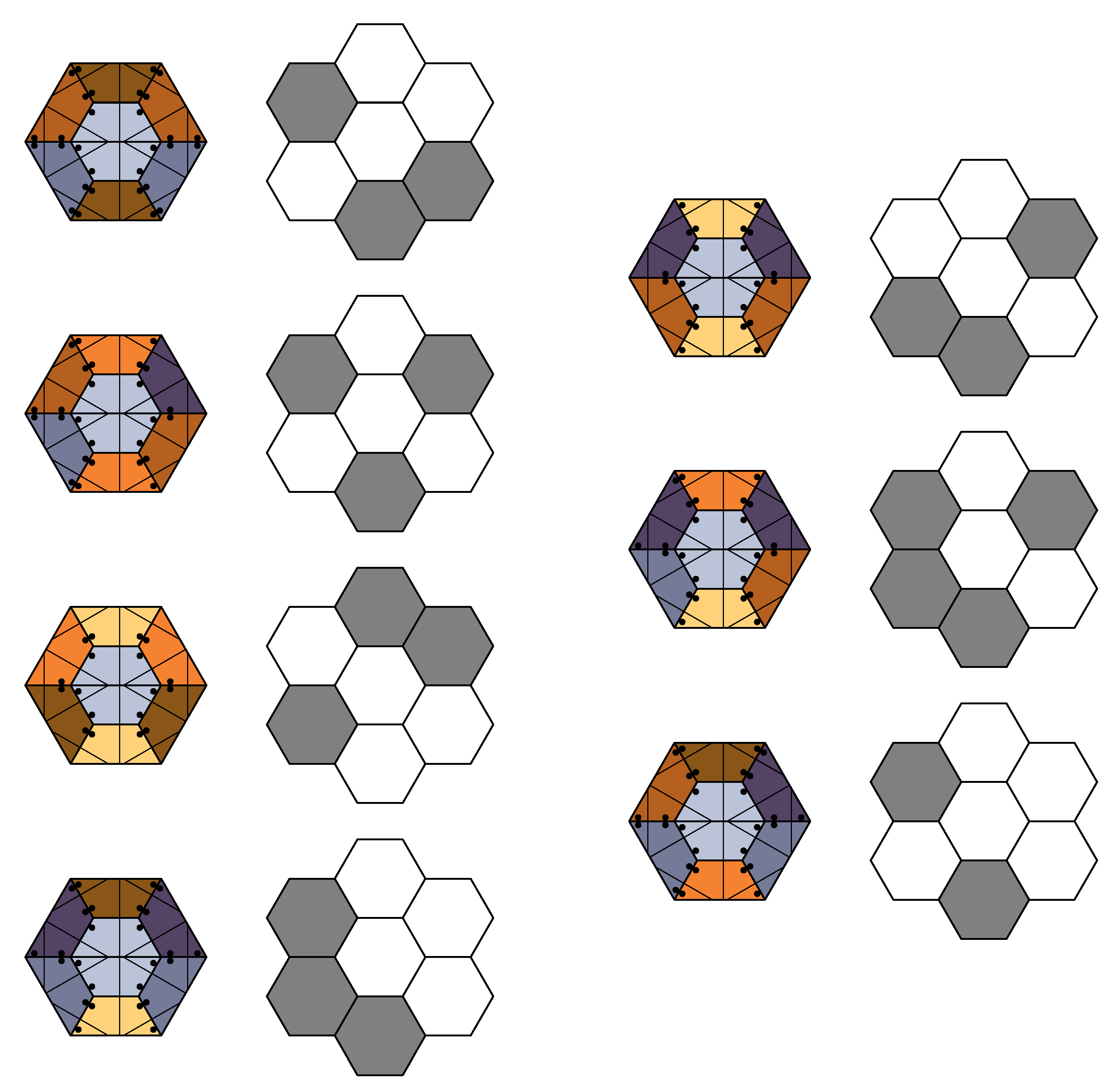
For the converse direction, there are three proofs known. The first is based on an idea by Joan Taylor, and is spelled out in detail in [26]. A related argument uses the local information contained in the llamas together with the correspondence of coloured and marked hexagons with local parity patterns, as indicated in Figure 9; see [9] for details. Finally, as for Theorem 1, one can reconstruct the complete decoration of any hexagon from the order-3 coronae of the llama tiling, which preserves the symmetry.
The final claim follows from the aperiodicity of the Taylor tiling by standard arguments. ☐
Figure 7.
The primitive inflation rule of Taylor’s half-hex inflation (top). The central patch of a fixed point tiling is shown on the lower left panel, with its parity pattern to the right.
Figure 7.
The primitive inflation rule of Taylor’s half-hex inflation (top). The central patch of a fixed point tiling is shown on the lower left panel, with its parity pattern to the right.
Before we continue with our general discussion, let us mention an interesting property of the llama tilings, which also holds for the Penrose parity pattern.
Figure 8.
Patch of a llama tiling, as derived from a fixed point tiling of the inflation rule of Figure 7. This particular pattern (and its infinite extension) possesses an almost colour reflection symmetry with respect to the indicated lines; see text for details.
Figure 8.
Patch of a llama tiling, as derived from a fixed point tiling of the inflation rule of Figure 7. This particular pattern (and its infinite extension) possesses an almost colour reflection symmetry with respect to the indicated lines; see text for details.

Theorem 3
Proof.
The patch of the Taylor tiling shown in Figure 8 is derived from one inflation fixed point with a hexagon (originally of type C) of positive chirality as a seed, which we denote as pattern P1. Another fixed point pattern, P2, can be obtained from the corresponding hexagon of opposite chirality, which has grey and white colours interchanged relative to P1. Nevertheless, P1 and P2 are LI, so that arbitrarily large patches of either pattern occur in the other.
Now, assume that P1 does not contain connected patches of white hexagons of unbounded size, where two hexagons are called connected when they share an edge. If so, there must be a maximal white “island” in P1, of diameter r say, which must then be surrounded by a connected “belt” of grey hexagons (which is possibly part of an even larger connected patch). Then, the same belt exists in P2, this time as a white belt around a grey island, and this belt has diameter by construction. Since P1 and P2 are LI, this patch from P2 must also occur somewhere in P1, in contradiction to the assumption, and our claim follows.
The argument for the Penrose parity pattern is completely analogous to that for the llama tilings, while the final claim is obvious. ☐
Figure 9.
Correspondence between fully decorated (half) hexagons, with central hexagon of type C, and their parity patterns.
Figure 9.
Correspondence between fully decorated (half) hexagons, with central hexagon of type C, and their parity patterns.
The llama tiling as well as Penrose’s parity pattern are thus interesting examples of deterministic aperiodic structures with percolation. In particular, an element with an infinite connected cluster must exist in either LI class. Since each class is a compact space, this claim follows from a compactness argument, because any sequence of tilings with connected clusters of increasing diameters around the origin must contain a subsequence that converges in the local topology to a tiling with an infinite cluster. Note, however, that the above argument does not imply the existence of a sequence of islands of growing size, which has been conjectured for the llama LI class [8] and seems equally likely in the other LI class as well, both on the basis of inflation series of suitable patches.
Between any Taylor tiling and the corresponding llama tiling (which are SMLD) is another version that still shows all line and point markings (and hence the chirality of the hexagons), but not the seven colours. Clearly, also this version, which we call the decorated llama tiling, is in the same SMLD class. One can now formulate three local rules for the corresponding prototile set, which consists of 12 tiles (up to translations).
- R1.
- The hexagons must match at common edges in the sense that the decoration lines do not jump on crossing the common edge;
- R2.
- The point markers must satisfy the edge transfer rule sketched in the middle panel of Figure 10, as indicated by the arrow, for any pair of hexagons separated by a single edge. The two points at the corners adjacent to that edge have to be in the same position, and this rule applies irrespective of the chirality types of the tiles;
- R3.
- No vertex configuration is allowed to have adjacent points in a threefold symmetric arrangement, such as the one shown in the right panel of Figure 10, or its rotated and reflected versions.
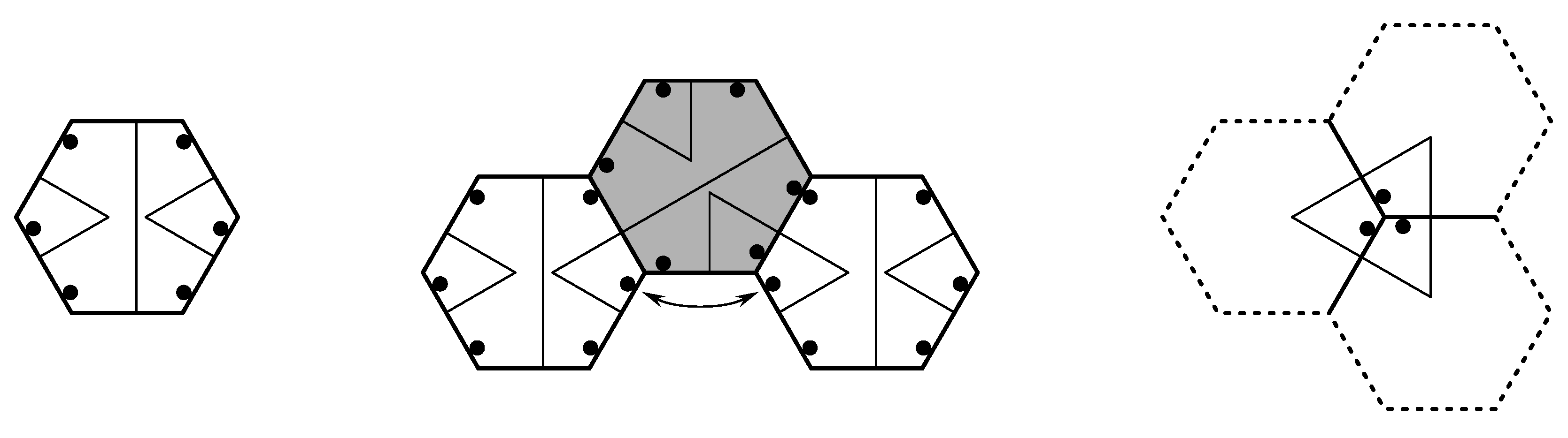
Figure 10.
Taylor’s functional monotile (left), a sketch of the edge transfer rule R2 (central) and the forbidden threefold vertex seed (right); see text for details.
Figure 10.
Taylor’s functional monotile (left), a sketch of the edge transfer rule R2 (central) and the forbidden threefold vertex seed (right); see text for details.

In [7,8], the following result is shown by the composition-decomposition method, with immediate consequences for other members of the corresponding MLD class.
Theorem 4
The rules R1–R3 constitute perfect aperiodic local rules for the LI class of the decorated llama tiling. Consequently, a corresponding set of perfect aperiodic local rules also exists for the LI class of the Taylor tilings and for the llama LI class. ☐
The decorated llama tiling was selected in the MLD class for the following reason.
Corollary 2
The hexagon of the left panel of Figure 10, together with its reflected copy, provides a functional monotile under the rules R1–R3. It defines the LI class of the decorated llama tiling. ☐
Let us mention that one can relax the three rules by omitting R3. As is proved in [8], this still provides a set of aperiodic local rules, this time for the larger space of the Socolar–Taylor tilings. This space is not minimal, and additionally contains two patterns with global threefold rotation symmetry (and their translates).
4. Topological Invariants and the Structure of the Hulls
In this section, we derive and compare further details of the hulls of the various hexagonal tilings, where we go beyond the material that has appeared in the literature so far. For this purpose, it proves useful to generate the tilings by lattice inflations in which the tiles are represented by the points of a triangular lattice, with the tile type attached as a label to each point. Geometrically, such lattice inflation tilings consist of labelled hexagon tiles only. Key tiles like the ones in the -tiling have to be absorbed into the type of the tiles (via suitable decorations).
When passing from half hexagons to full hexagons, one easily obtains the overlapping inflation (also called pseudo inflation) shown in Figure 11 (left) for the half-hex tiling. The outer ring of hexagons is shared between the inflations of neighbouring hexagons. A pseudo inflation has to be consistent in the sense that it agrees on the overlap regions. From this pseudo inflation, a standard inflation can be obtained by replacing each hexagon by the four shaded hexagons only, independently of the orientation of the original hexagon. Conversely, each hexagon in the inflated tiling is assigned to a unique supertile hexagon. The inflation rule obtained in this way is not rotation covariant, but this is only a minor disadvantage. Also, the fixed point tiling obtained under the iterated inflations no longer covers the entire plane, but only a 120-degree wedge, which is not a problem either. Since the inflation rule is derived from a pseudo inflation, it determines the tiling also in the other sectors, and there is a unique continuation to the rest of the plane. Technically speaking, the inflation rule forces the border [27], a property that simplifies the computation of topological invariants considerably.
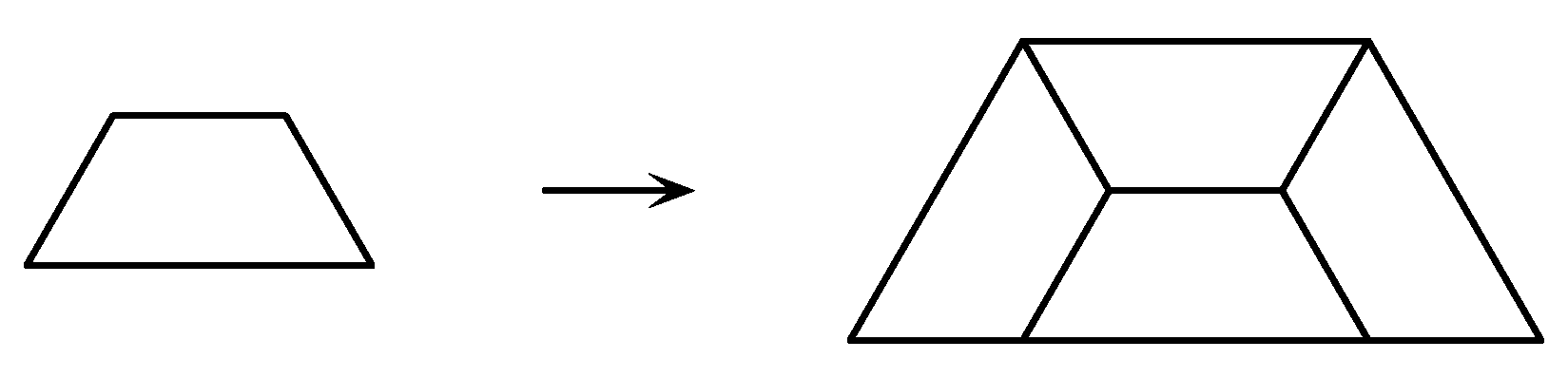
Figure 11.
Hexagon (pseudo) inflation for the half-hex (left) and for two (locally equivalent) variants of the arrowed half-hex (centre and right). If only the shaded hexagons are retained, a standard inflation for a wedge with opening angle is obtained; see text for details.
Figure 11.
Hexagon (pseudo) inflation for the half-hex (left) and for two (locally equivalent) variants of the arrowed half-hex (centre and right). If only the shaded hexagons are retained, a standard inflation for a wedge with opening angle is obtained; see text for details.
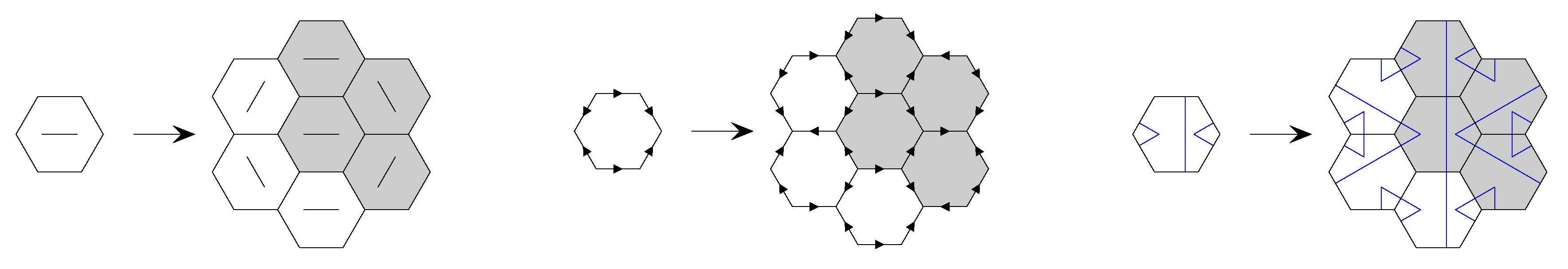
A natural generalisation of the half-hex tiling is the arrowed half-hex tiling, obtained by either of the two variants of (pseudo) inflations shown in Figure 11 (centre and right). Clearly, the two decorations are locally equivalent and lead to tilings that are MLD. Just as for the half-hex, a pseudo inflation is obtained first, from which a standard inflation is then derived by taking only the shaded tiles. The arrow pattern on the hexagons shown in Figure 11 (centre) is the same as that of the hexagon tile of the -tiling. In fact, it is easy to see that the arrowed half-hex is locally derivable from the latter, and thus is a factor. Similarly, the hexagon decoration of Figure 11 (right) is part of the decoration of the Taylor hexagons, so that the arrowed half-hex is also a factor of the Taylor tiling.
Corollary 3
The hull of the half-hex tiling, viewed as a dynamical system under the action of , is a topological factor of both the -tiling hull and the Taylor tiling hull. The same property holds for the hull of the arrowed half-hex tiling. ☐
A larger patch of the arrowed half-hex tiling is shown in Figure 12 (in the Taylor decoration variant). The fixed point tilings generated from the six different orientations of the arrowed hexagon differ only along three rows of hexagons crossing in the centre of the figure. We call these the singular rows. The six fixed point tilings project to the same point on the solenoid . Moreover, pushing the fixed point centre along one of the singular rows towards infinity, pairs of tilings that are mirror images of each other are obtained, except on the one singular row that remains. Each such pair of tilings also projects to the same points of the solenoid . In fact, each singular row gives rise to a 1d sub-solenoid , onto which the projection is 2-to-1 (except for the crossing point of these sub-solenoids). Three such sub-solenoids , onto which the projection is 2-to-1, clearly exist in the -tiling and in the Taylor tiling as well. However, for the (naked) half-hex tiling, there are no singular rows. In this case, there are just three fixed point tilings, differing in the orientation of the central hexagon only, which project to the same point on the solenoid . We refer to [9] for an explicit derivation of the model set coordinates of the arrowed half-hex tiling.
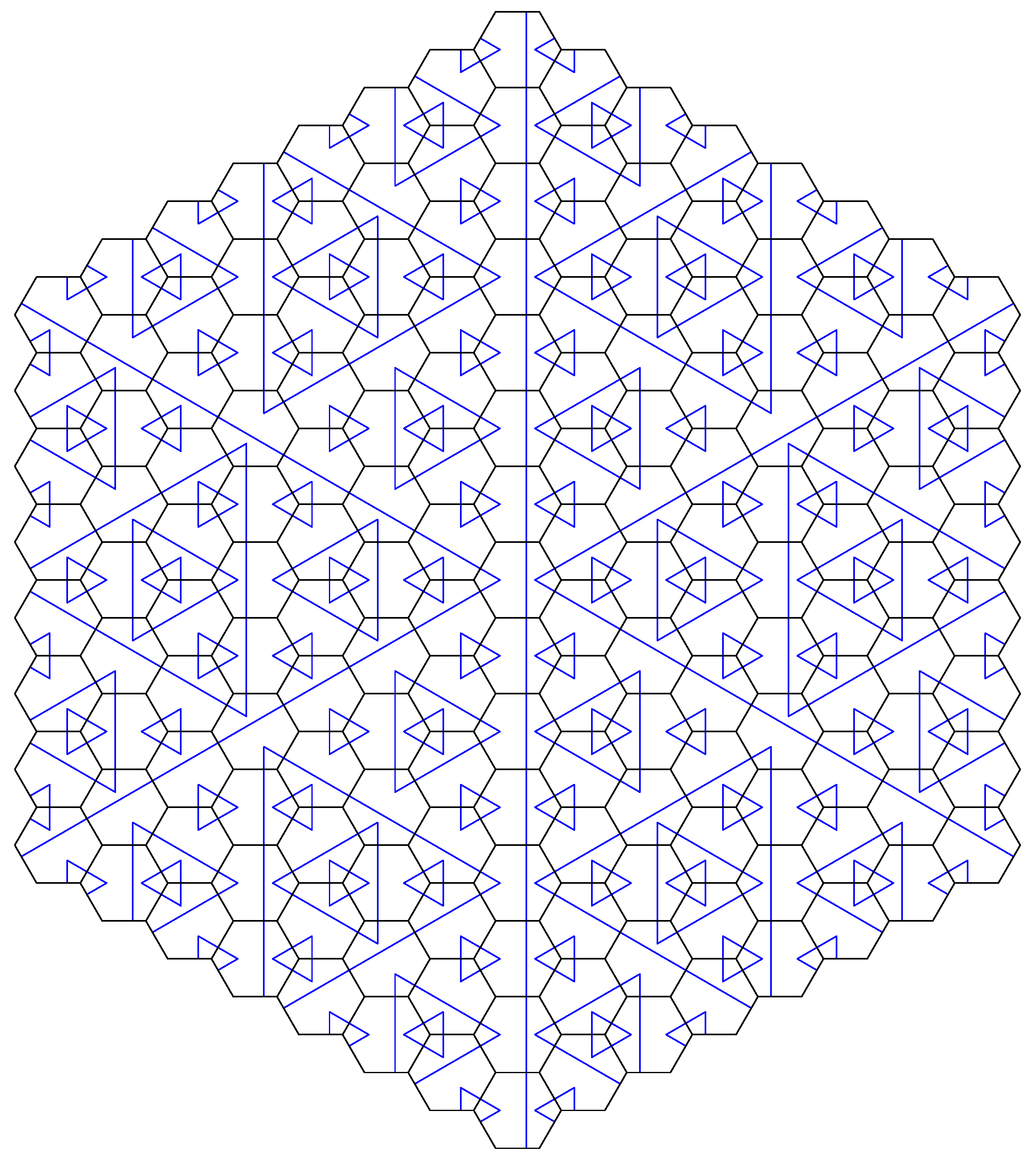
Figure 12.
Patch of the arrowed half-hex tiling. The blue decoration lines form an infinite hierarchy of triangles of all sizes. The blue triangles of a given size and orientation form a triangular lattice.
Figure 12.
Patch of the arrowed half-hex tiling. The blue decoration lines form an infinite hierarchy of triangles of all sizes. The blue triangles of a given size and orientation form a triangular lattice.

The hexagon of the arrowed half-hex tiling has still one remaining line of mirror symmetry. Both the -tiling and the Taylor tiling break this remaining symmetry, alongside with a splitting into 7 subtypes of hexagons, which differ in their behaviour under the inflation. For the Taylor tiling, a pseudo inflation for fully asymmetric hexagons follows easily from Figure 7, which can then be converted into a standard lattice inflation as before.
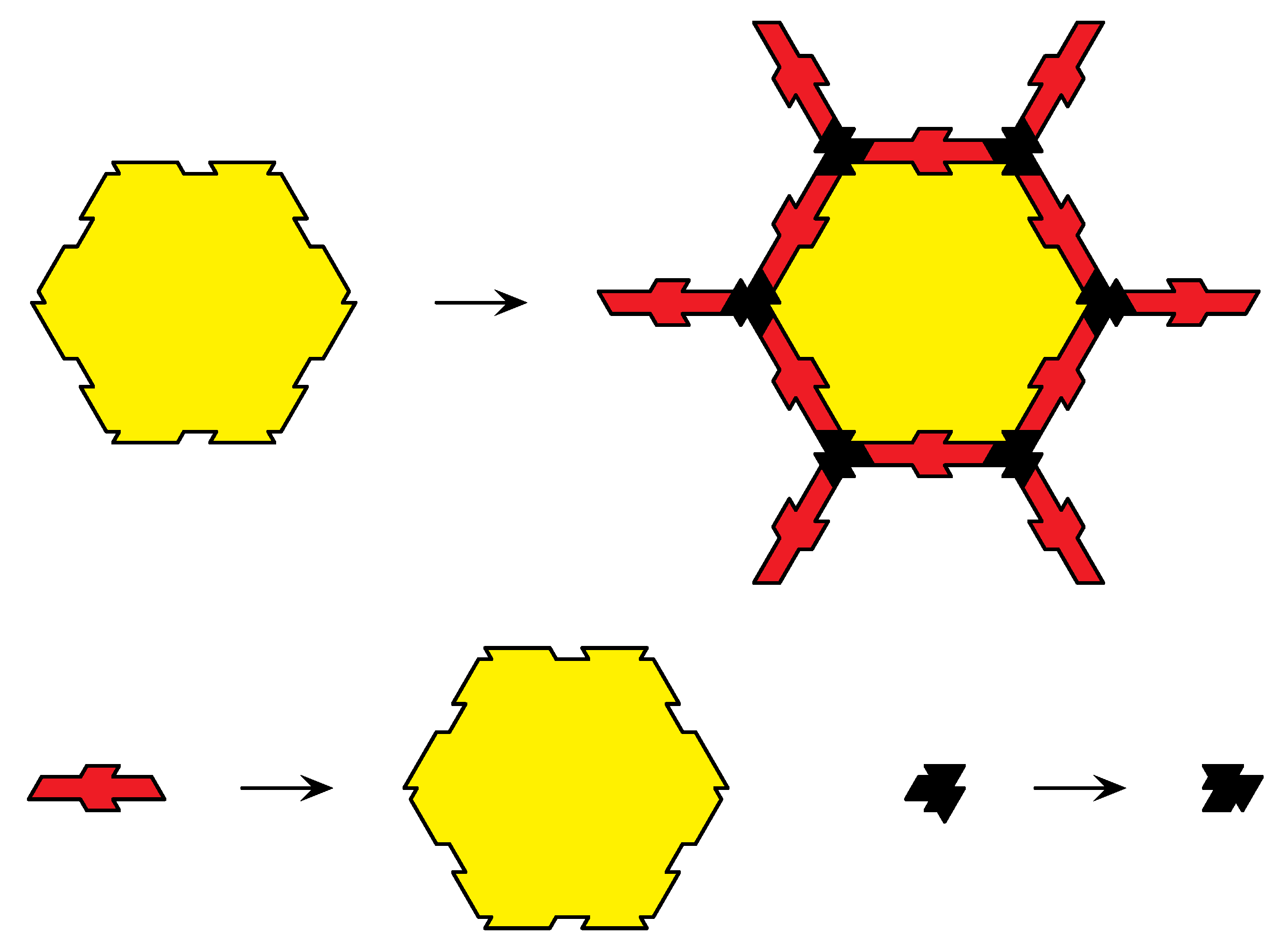
For the -tiling, we replace the ε- and -tiles by the equivalent line decoration for the hexagons shown in Figure 13, which was introduced already in [6]. In addition to the blue lines of the arrowed half-hex, which encode the arrows of the ε-tiles along the hexagon edges, there is now also a second set of red lines, which encode the information contained in the -tiles and in the asymmetry across the ε-tiles. The latter is represented by the piece of red line parallel to the hexagon edge. The matching condition of the -tiles is replaced by the requirement that red lines must continue across tile edges. In the interior, each hexagon carries an X-shaped pair of red line angles, and a red line belt, which breaks the remaining mirror symmetry of the blue line decoration. The inflation rule for the 7 types of decorated hexagons is shown in Figure 14.
Figure 13.
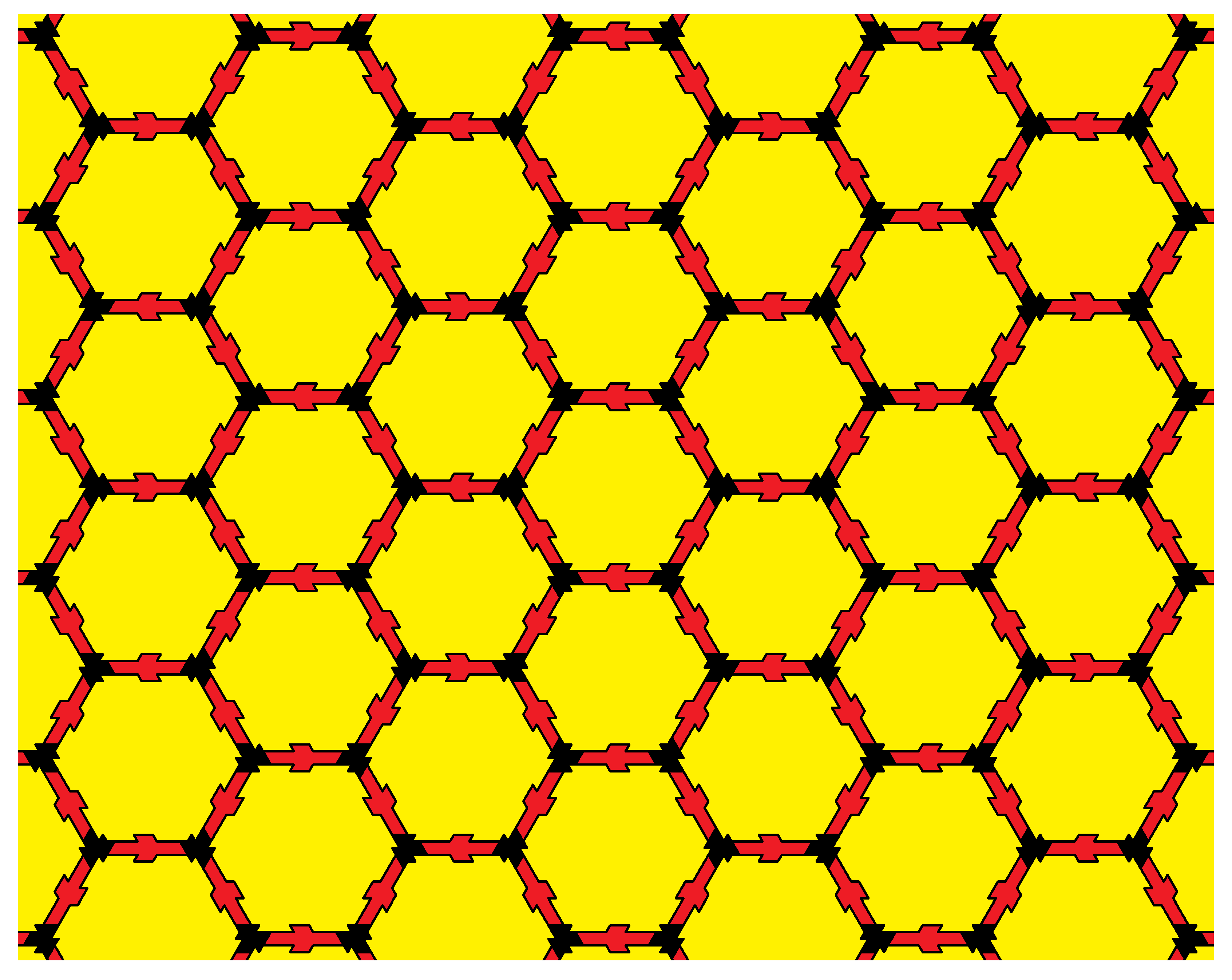
Patch of the -tiling in the variant with line decorations. In addition to the hierarchy of blue triangles from the half-hex tiling, there is now also a hierarchy of red hexagons. Hexagons of each size form a lattice periodic array, with lattices of different densities.
Figure 13.
Patch of the -tiling in the variant with line decorations. In addition to the hierarchy of blue triangles from the half-hex tiling, there is now also a hierarchy of red hexagons. Hexagons of each size form a lattice periodic array, with lattices of different densities.
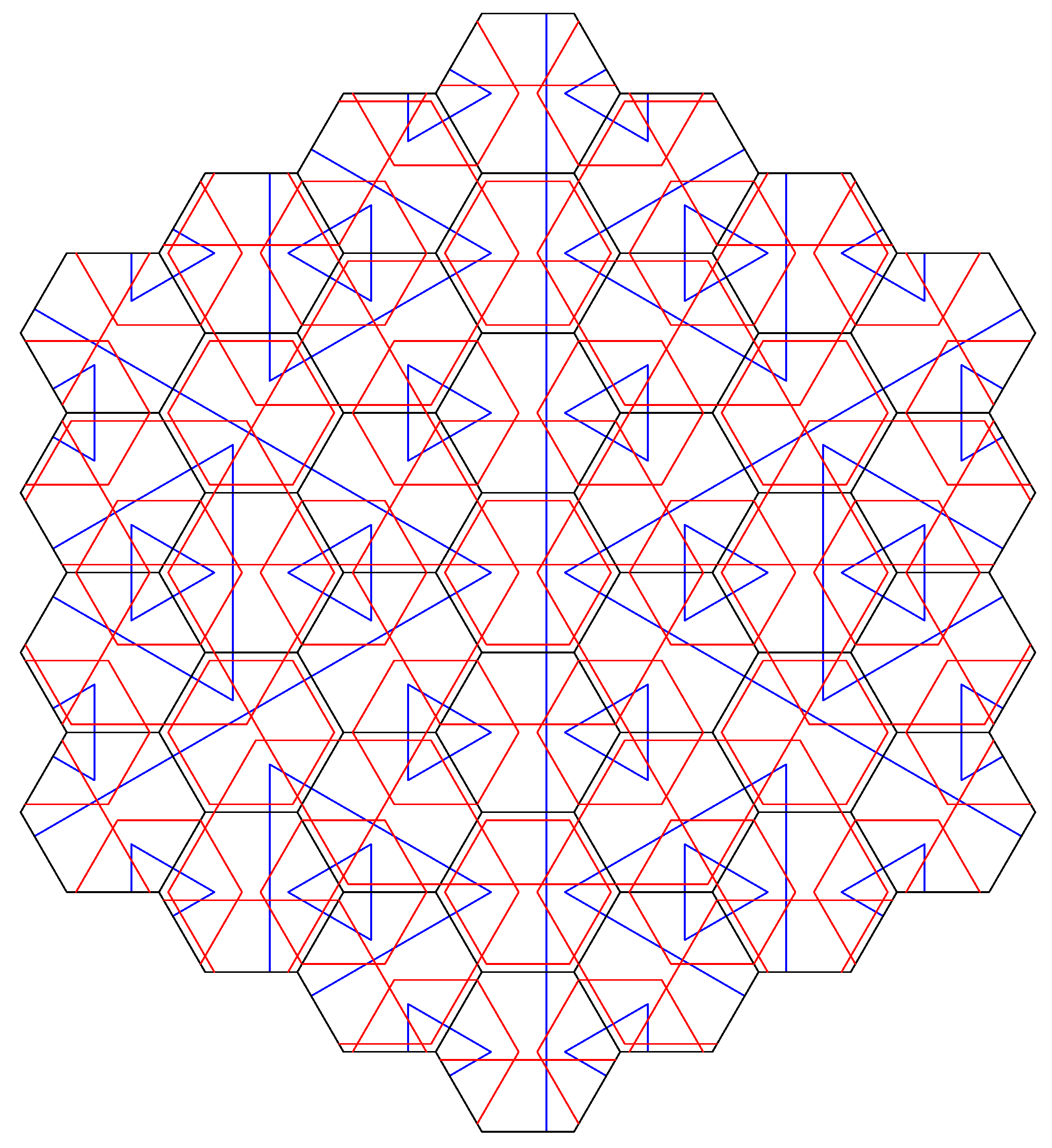
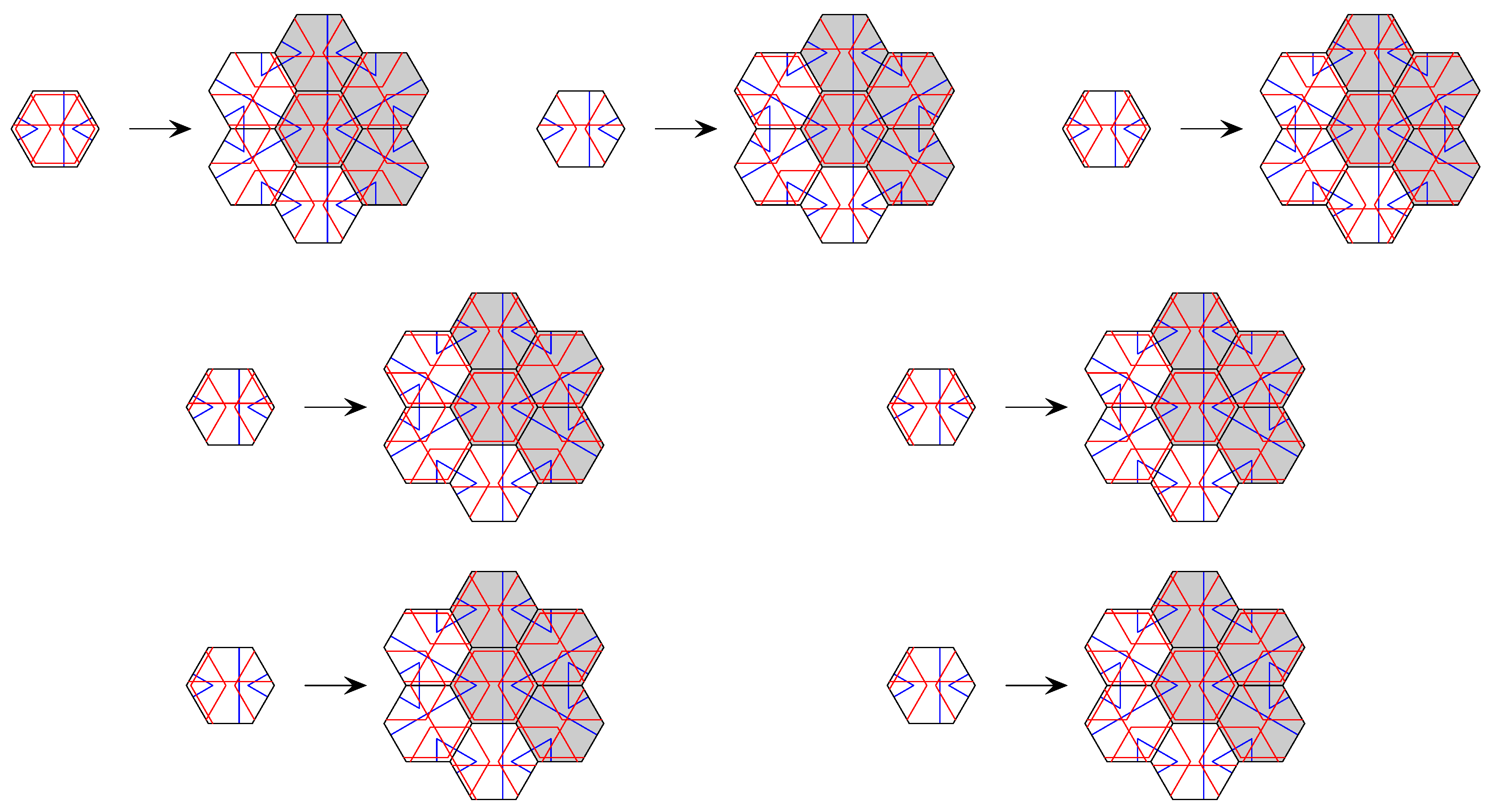
Figure 14.
Inflation rules for -tiling in the variant with line decorations. If a hexagon is replaced by 7 hexagons, a pseudo inflation is obtained. Taking only the 4 shaded hexagons results in a standard inflation rule (for one sector).
Figure 14.
Inflation rules for -tiling in the variant with line decorations. If a hexagon is replaced by 7 hexagons, a pseudo inflation is obtained. Taking only the 4 shaded hexagons results in a standard inflation rule (for one sector).
From Figure 13, it is clear that the red line decoration breaks the horizontal mirror symmetry of the blue arrowed half-hex decoration. Therefore, there will be three additional 1d sub-solenoids in three further directions, to which the projection is 2-to-1 rather than 1-to-1. These 1d solenoids, as well as those of the arrowed half-hex, all intersect in the single point to which the now 12 fixed point tilings project. Moreover, the three “red” sub-solenoids intersect also in two further points at corners of the hexagons, which are fixed points under the square of the inflation. On these points, the projection to the solenoid is 6-to-1.
The set of points on the solenoid to which the projection of the Taylor tiling is not 1-to-1 is completely analogous. The corresponding ambiguities of the decoration, starting with a fixed point tiling with full or symmetry, has been derived in [8]. For an independent approach, see [26]. A summary of the projection situation is sketched and explained in Figure 15.
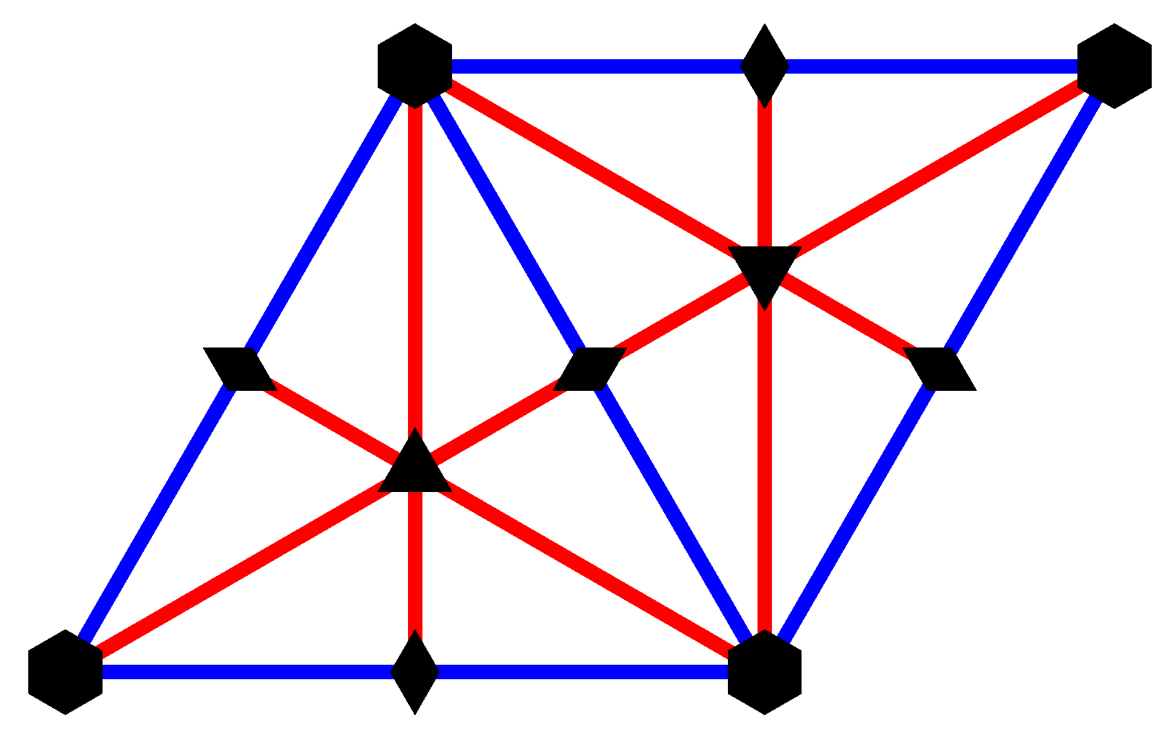
Figure 15.
Schematic representation of the hulls of the different hexagon tilings via a (closed) toral slice of the underlying solenoid. The projection fails to be 1-to-1 on the lines as follows. For the half-hex, the projection is 3-to-1 precisely at the points marked by a hexagon, and 1-to-1 elsewhere. For the arrowed half-hex, the 1d sub-solenoids where the projection is 2-to-1 are shown as blue lines. At the hexagon points, three blue sub-solenoids intersect, and the projection is 6-to-1. For the Taylor and the Penrose hexagon tilings, there are three additional sub-solenoids (red lines) along which the projection is 2-to-1. These intersect at two inequivalent points (marked by triangles) where the projection is 6-to-1 (at such points, three infinite order supertiles meet). The projection is 12-to-1 at the hexagon points (which are centres of infinite-order supertiles). Note that, at the points marked by diamonds, not only two but in fact all six sub-solenoids intersect. This is due to the dyadic structure of the hull. As these points have half-integer coordinates with respect to the hexagonal lattice, they are equivalent (in the solenoid) to the points marked by hexagons.
The first benefit of having represented all four tilings as lattice inflations is the following.
Theorem 5
The half-hex, arrowed half-hex, and Taylor tilings are all model sets, and as such have pure point dynamical and diffraction spectrum.
Sketch of Proof.
As the half-hex and arrowed half-hex tilings are both factors of the other two tilings, we only need to consider the - and Taylor tilings. Both have one “preferred” tile type, which occurs twice as often as the other tile types. For the Taylor tiling, it is type C (light blue in Figure 7), and for the -tiling it is the first type in Figure 14. In both cases, the centres of the preferred tiles form a triangular sublattice of index 4. Also the supertiles (of any fixed order) of the preferred tile types form a periodic array (disregarding orientation). Moreover, the preferred tiles are the seeds of the 12 fixed point tilings, which differ from each other only along the 6 mirror lines of the symmetry group. A sufficiently high order supertile therefore contains tiles which are the same in all preferred supertiles, independently of their orientation. Therefore, any Taylor or -tiling contains a lattice-periodic subset of tiles. The results of Theorem 3 from [3] then imply that they must be model sets and hence have pure point dynamical and diffraction spectrum by [15]. ☐
Another benefit of dealing with a lattice inflation is that the Anderson–Putnam approach [27] to computing the Čech cohomology of the hull becomes relatively easy to implement, since tiles are represented as labelled lattice points whose environments are easy to determine. Moreover, as the lattice inflation rules are derived from overlapping pseudo inflation rules, they have the property of forcing the border, which allows one to avoid the complication of using collared tiles; see [27] for details.
In this approach, from the local environments of the tiling a finite approximant cell complex is constructed, whose points represent cylinder sets of tilings. The full tiling space is then obtained as the inverse limit space of the inflation acting on the approximant cell complex. Correspondingly, the Čech cohomology of the hull is the direct limit of the inflation action on the cohomology of the approximant complex. For further details, we refer to [27,28]; compare also [20] for some explicitly worked-out examples. For our four tiling spaces, the following results are obtained.
Theorem 6
The four hexagon tiling spaces have the following Čech cohomologies:
In particular, the -groups are distinct. ☐
Since the - and the Taylor tiling have different cohomology, it immediately follows that they cannot be in the same MLD class.
Corollary 4
The LI class and the Taylor LI class define distinct MLD classes. ☐
As a side result of the cohomology calculation, the Artin–Mazur dynamical zeta function of the inflation action on the hull can also be obtained. It is defined as
where is the number of points in the hull invariant under an m-fold inflation. We note that, if the hull consists of two (or more) components for which the periodic points can be counted separately, , the corresponding partial zeta functions have to be multiplied: . This will turn out to be useful shortly. For the action of the mapping on the dyadic solenoids and , the zeta function coincides with that of the corresponding toral endomorphism, which are
by an application of the results from [29]. The corresponding fixed point counts read and , for .
Anderson and Putnam [27] have shown that the dynamical zeta function can be computed from the action of the inflation on the cochain groups of the approximant complex. Here, we rather express it in terms of the action of the inflation on the rational cohomology groups of the hull. If is the matrix of the inflation action on the m-th rational cohomology group, the dynamical zeta function is given by
where the latter equality holds when the matrices are diagonalisable with eigenvalues . The additional terms in the expressions from [27] cancel between numerator and denominator.
From the cohomology and the eigenvalues , the dynamical zeta function is easily obtained. For the half-hex, we get
which we have written as the product of the zeta function of the 2d solenoid and the generating function of two additional fixed points. This is in line with our observation that the projection to is 1-to-1 except at one point, where it is 3-to-1, wherefore there are two extra fixed points beyond the one already present in .
For the arrowed half-hex, we find
which is the product of the zeta functions of a 2d solenoid , three 1d solenoids , and two additional fixed points. As discussed above, we have three 1d solenoids where the projection to is 2-to-1, hence the three extra copies of . The projection from the fixed points of the arrowed half-hex tiling is 6-to-1 (they form a -orbit), so that there must be two extra fixed points in the zeta function, in addition to those contained in the 4 solenoids.
Finally, both for the - and the Taylor tilings, we obtain
which is the product of the zeta functions of a 2d solenoid , six 1d solenoids , five additional fixed points, and two extra 2-cycles. Even though the two tilings have different cohomology, the additional terms in the zeta function of the Taylor tiling (indicated by the extra exponents in parentheses) cancel each other. As discussed above, both hulls contain six 1d solenoids onto which the projection is 2-to-1. The 12 fixed points, forming a -orbit, all project to the same point, where the six 1d sub-solenoids intersect. In addition to the 7 fixed points in the altogether 7 solenoids, there must hence be 5 further fixed points, which indeed show up in the zeta function. Finally, the three “red” 1d solenoids intersect also at two types of corners of the hexagon tiles. These points form 2-cycles under the inflation, and the projection to them is 6-to-1 (two -orbits). Hence, two extra 2-cycles are present in the zeta function. The zeta functions derived above confirm that our analysis of the set where the projection to fails to be 1-to-1 must have been complete.
Corollary 5
The corresponding fixed point counts, for , are given by , by , and by . ☐
It is a rather amazing fact that the Penrose and the Taylor tiling, despite defining distinct MLD classes, share the same dynamical zeta function for the respective inflation action, and have a projection to the 2d solenoid with exactly the same multiplicities.
5. Outlook and Open Problems
The two tiling spaces due to Penrose and due to Taylor, which are both model sets (see also [26]), show amazing similarities, though they are certainly not MLD. Whether there is a local derivation in one direction is still not fully clear, but unlikely. It is an open problem where and what exactly is the difference between the two tilings.
In the two parity patterns, beyond the percolation structure, one can see islands of growing size in both tilings. Based on the inflation structure, it is thus natural to conjecture that both classes of parity patterns contain islands of unbounded size, though a proof does not seem obvious. Also, the emergence via inflation series seems slightly different in the two tilings.
The quest for a true monotile in the plane is not settled yet, because the rules cannot be realised by nearest neighbour conditions, and hence not by simple markings alone (unless one admits a prototile version with disconnected parts). There are other attempts to find an example, for instance via polyominoes and related objects; compare [30] and references therein.
An entirely different situation is met in 3-space, where the famous SCD prototile [31,32] establishes a mechanism that is truly three-dimensional. Indeed, the non-periodicity here is a result of a screw axis with an incommensurate rotation, wherefore the repetitive cases are aperiodic, but not strongly aperiodic; see [4] for a discussion. Also, unlike the situation above, the local rules for the SCD tile have to explicitly exclude the use of a reflected version, which is perhaps not fully satisfactory either.
In summary, some progress was made in the quest for an aperiodic monotile in recent years, but the search is certainly not over yet!
Acknowledgments
We are grateful to Roger Penrose and Joan Taylor for important comments and suggestions, to Robert Moody and Egon Schulte for helpful discussions, and to two anonymous reviewers for various constructive comments. This work was supported by the German Research Council (DFG), within the CRC 701. UG is grateful to the Fields Institute for financial support.
References
- Grünbaum, B.; Shephard, G.C. Tilings and Patterns; Freeman: New York, NY, USA, 1987. [Google Scholar]
- Frettlöh, D.; Sing, B. Computing modular coincidences for substitution tilings and point sets. Discrete Comput. Geom. 2007, 37, 381–407. [Google Scholar] [CrossRef]
- Lee, J.-Y.; Moody, R.V. Lattice substitution systems and model sets. Discrete Comput. Geom. 2001, 25, 173–201. [Google Scholar] [CrossRef]
- Baake, M.; Grimm, U. On the notions of symmetry and aperiodicity for Delone sets. Symmetry 2012, 4, 566–580. [Google Scholar] [CrossRef]
- Goodman-Strauss, C. Matching rules and substitution tilings. Ann. Math. 1998, 147, 181–223. [Google Scholar] [CrossRef]
- Penrose, R. Remarks on tiling: Details of a (1 + ε + ε2)-aperiodic set. In the Mathematics of Long-Range Aperiodic Order; Moody, R.V., Ed.; NATO ASI series 489; Kluwer: Dordrecht, the Netherlands, 1997; pp. 467–497. [Google Scholar]
- Taylor, J.M. Aperiodicity of a functional monotile. Available online: http://www.math.uni-bielefeld.de/sfb701/preprints/view/420 (accessed on 16 October 2012).
- Socolar, J.E.S.; Taylor, J.M. An aperiodic hexagonal tile. J. Comb. Theory A 2011, 118, 2207–2231. [Google Scholar] [CrossRef]
- Baake, M.; Grimm, U. Theory of Aperiodic Order: A Mathematical Invitation; Cambridge University Press: Cambridge, UK, in preparation.
- Moody, R.V. Meyer sets and their duals. In the Mathematics of Long-Range Aperiodic Order; Moody, R.V., Ed.; NATO ASI series 489; Kluwer: Dordrecht, the Netherlands, 1997; pp. 403–441. [Google Scholar]
- Moody, R.V. Model sets: A survey. In from Quasicrystals to More Complex Systems; Axel, F., Dénoyer, F., Gazeau, J.P., Eds.; Springer: Berlin, Germany, 2000; pp. 145–166. [Google Scholar]
- Frettlöh, D. Nichtperiodische Pflasterungen mit ganzzahligem Inflationsfaktor. Ph.D. thesis, University Dortmund, Dortmund, Germany, 2002. [Google Scholar]
- Gähler, F.; Klitzing, R. The diffraction pattern of self-similar tilings. In the Mathematics of Long-Range Aperiodic Order; Moody, R.V., Ed.; NATO ASI series 489; Kluwer: Dordrecht, the Netherlands, 1997; pp. 141–174. [Google Scholar]
- Baake, M.; Lenz, D. Dynamical systems on translation bounded measures: Pure point dynamical and diffraction spectra. Ergod. Theory Dyn. Syst. 2004, 24, 1867–1893. [Google Scholar] [CrossRef]
- Lee, J.-Y.; Moody, R.V.; Solomyak, B. Pure point dynamical and diffraction spectra. Ann. Henri Poincaré 2002, 3, 1003–1018. [Google Scholar] [CrossRef]
- Schlottmann, M. Generalised model sets and dynamical systems. In Directions in Mathematical Quasicrystals; Baake, M., Moody, R.V., Eds.; AMS: Providence, RI, USA, 2000; pp. 143–159. [Google Scholar]
- Baake, M.; Moody, R.V. Weighted Dirac combs with pure point diffraction. J. Reine Angew. Math. (Crelle) 2004, 573, 61–94. [Google Scholar] [CrossRef]
- Baake, M.; Schlottmann, M.; Jarvis, P.D. Quasiperiodic patterns with tenfold symmetry and equivalence with respect to local derivability. J. Phys. A 1991, 24, 4637–4654. [Google Scholar] [CrossRef]
- Baake, M. A guide to mathematical quasicrystals. In Quasicrystals—An Introduction to Structure, Physical Properties and Applications; Suck, J.-B., Schreiber, M., Häussler, P., Eds.; Springer: Berlin, Germany, 2002; pp. 17–48. [Google Scholar]
- Baake, M.; Gähler, F.; Grimm, U. Spectral and topological properties of a family of generalised Thue-Morse sequences. J. Math. Phys. 2012, 53, 032701:1–24. [Google Scholar]
- Baake, M.; Gähler, F.; Grimm, U. Examples of substitution systems and their factors. Unpublished work. 2012. [Google Scholar]
- Gähler, F. Substitution rules and topological properties of the Robinson tilings. Unpublished work. 2012. [Google Scholar]
- Gähler, F. Matching rules for quasicrystals: The composition-decomposition method. J. Non-Cryst. Solids 1993, 153–154, 160–164. [Google Scholar] [CrossRef]
- Penrose, R. Supplement to remarks on tiling: Details of a (1 + ε + ε2)-aperiodic set. In Roger Penrose Collected Works; Oxford University Press: Oxford, UK, 2011; Volume 6. [Google Scholar]
- Baake, M.; Lenz, D.; Moody, R.V. Characterisation of model sets by dynamical systems. Ergod. Theory Dyn. Syst. 2007, 27, 341–382. [Google Scholar] [CrossRef]
- Lee, J.-Y.; Moody, R.V. Taylor-Socolar hexagonal tilings as model sets. Symmetry 2012. submitted for publication. [Google Scholar] [CrossRef]
- Anderson, J.E.; Putnam, I.F. Topological invariants for substitution tilings and their associated C*-algebras. Ergod. Theory Dyn. Syst. 1998, 18, 509–537. [Google Scholar] [CrossRef]
- Sadun, L. Topology of Tiling Spaces; AMS: Providence, RI, USA, 2008. [Google Scholar]
- Baake, M.; Lau, E.; Paskunas, V. A note on the dynamical zeta function of general toral endomorphisms. Monatsh. Math. 2009, 161, 33–42. [Google Scholar] [CrossRef]
- Rhoads, G.C. Planar tilings by polyominoes, polyhexes, and polyiamonds. J. Comput. Appl. Math. 2005, 174, 329–353. [Google Scholar]
- Baake, M.; Frettlöh, D. SCD patterns have singular diffraction. J. Math. Phys. 2005, 46, 033510:1–10. [Google Scholar] [CrossRef]
- Danzer, L. A family of 3D-spacefillers not permitting any periodic or quasiperiodic tiling. In Aperiodic ’94; Chapuis, G., Paciorek, W., Eds.; World Scientific: Singapore, 1995; pp. 11–17. [Google Scholar]
© 2012 by the authors licensee MDPI, Basel, Switzerland. This article is an open access article distributed under the terms and conditions of the Creative Commons Attribution license ( http://creativecommons.org/licenses/by/3.0/).
Share and Cite
MDPI and ACS Style
Baake, M.; Gähler, F.; Grimm, U. Hexagonal Inflation Tilings and Planar Monotiles. Symmetry 2012, 4, 581-602. https://doi.org/10.3390/sym4040581
AMA Style
Baake M, Gähler F, Grimm U. Hexagonal Inflation Tilings and Planar Monotiles. Symmetry. 2012; 4(4):581-602. https://doi.org/10.3390/sym4040581
Chicago/Turabian StyleBaake, Michael, Franz Gähler, and Uwe Grimm. 2012. "Hexagonal Inflation Tilings and Planar Monotiles" Symmetry 4, no. 4: 581-602. https://doi.org/10.3390/sym4040581