Topological Many-Body States in Quantum Antiferromagnets via Fuzzy Supergeometry

Abstract
:
1. Introduction

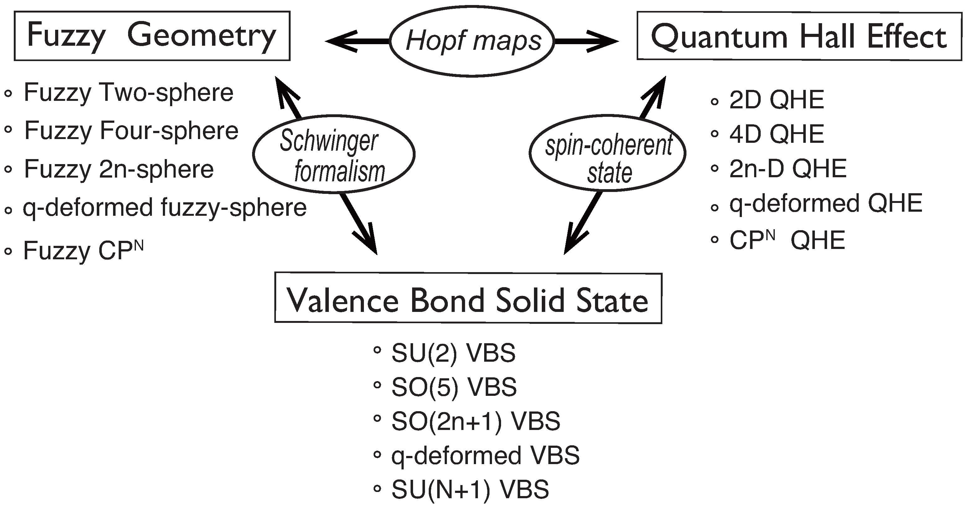
2. Fuzzy Geometry and Valence Bond Solid States
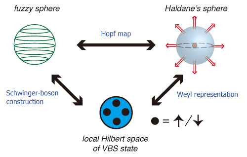
2.1. Fuzzy Two-Spheres and the Lowest Landau Level Physics
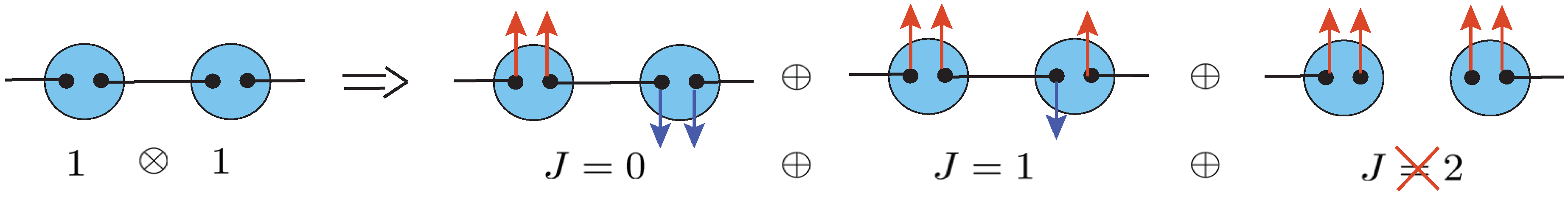
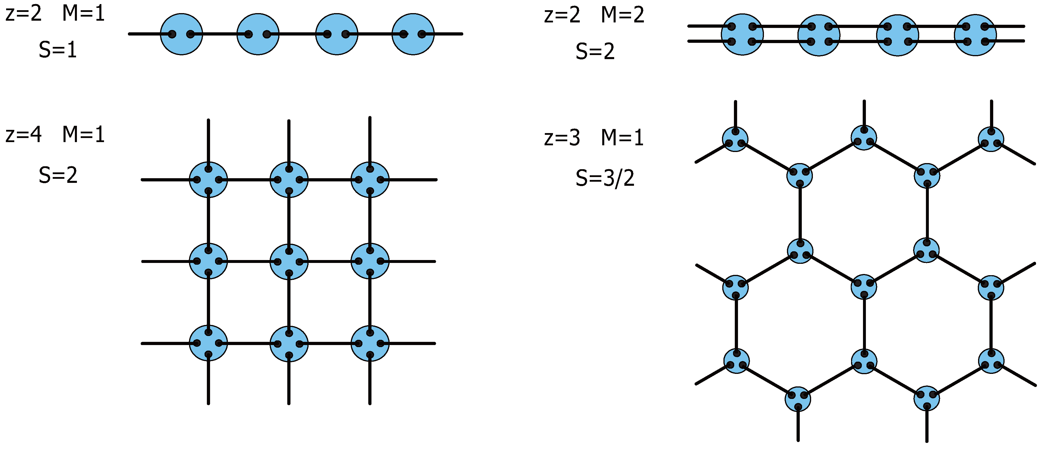
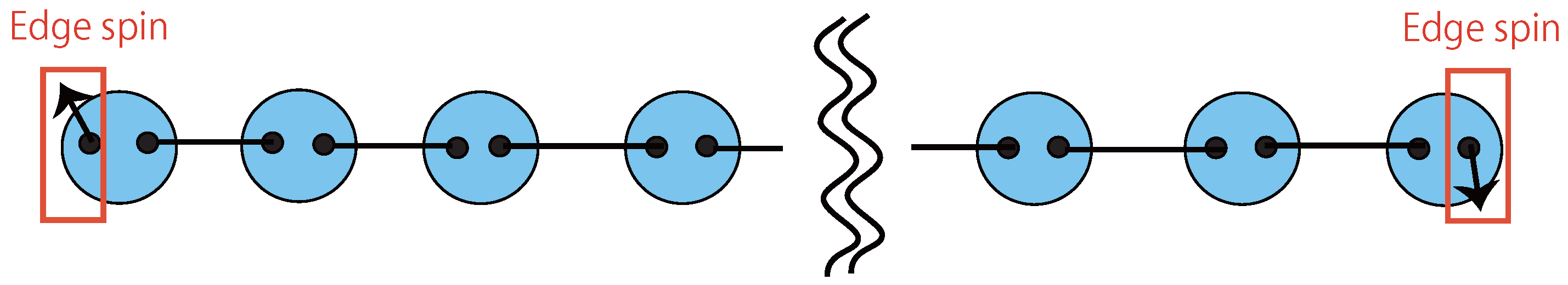
2.2. Valence Bond Solid States


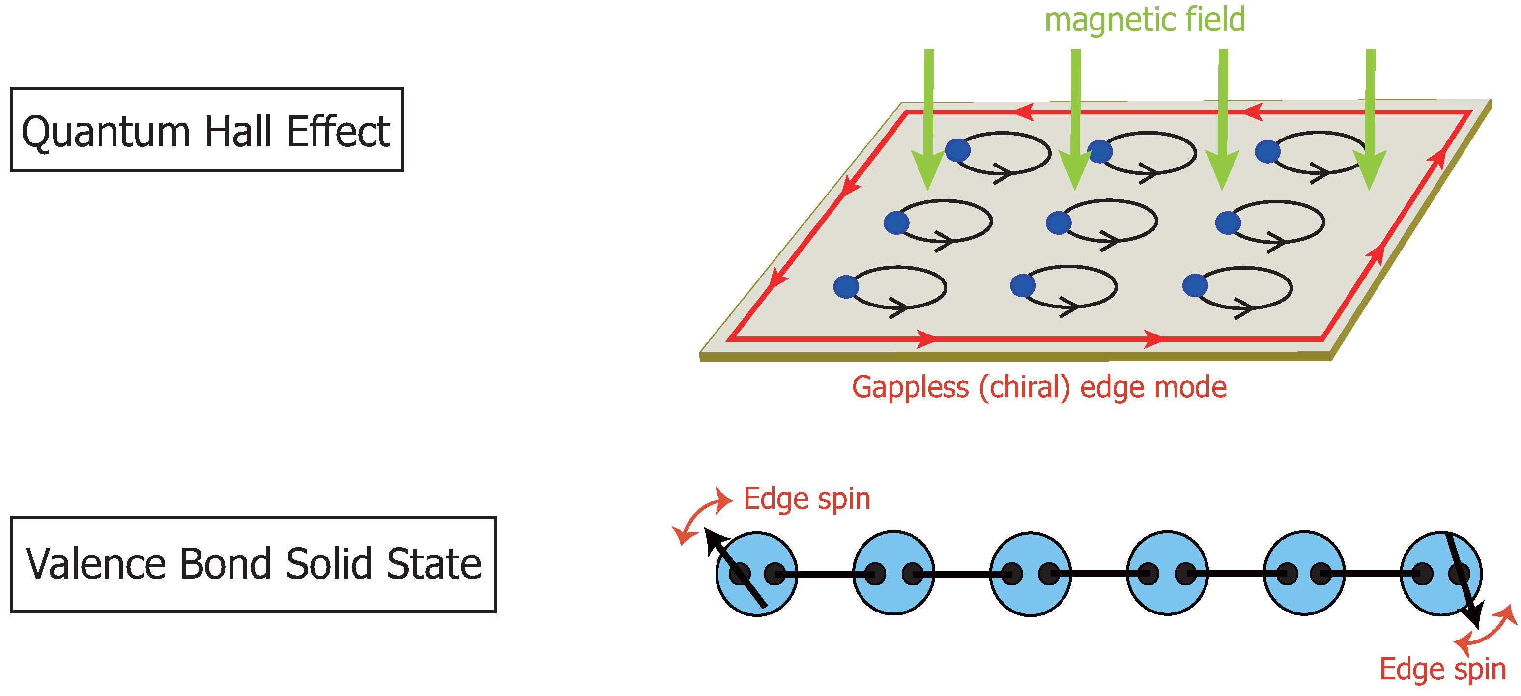
| QHE | QAFM | |
|---|---|---|
| Many-body state | Laughlin-Haldane wave function | VBS state |
| Power | m: inverse of filling factor | M: number of VBs between neighboring sites |
| Charge | : monopole charge | : local spin magnitude |
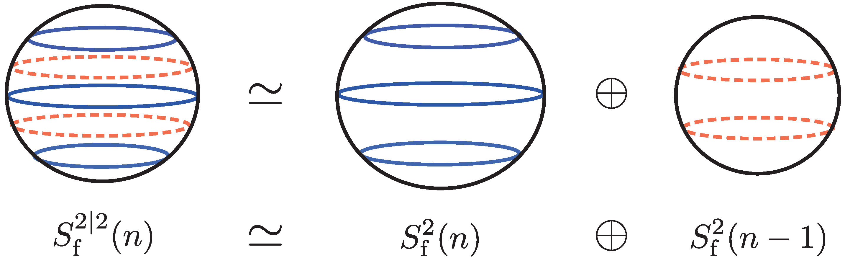
3. Fuzzy Two-Supersphere
3.1.

3.2.
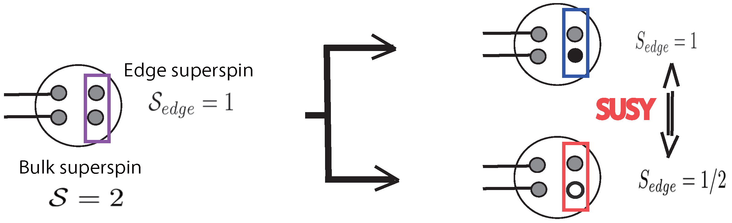
4. Supersymmetric Valence Bond Solid States
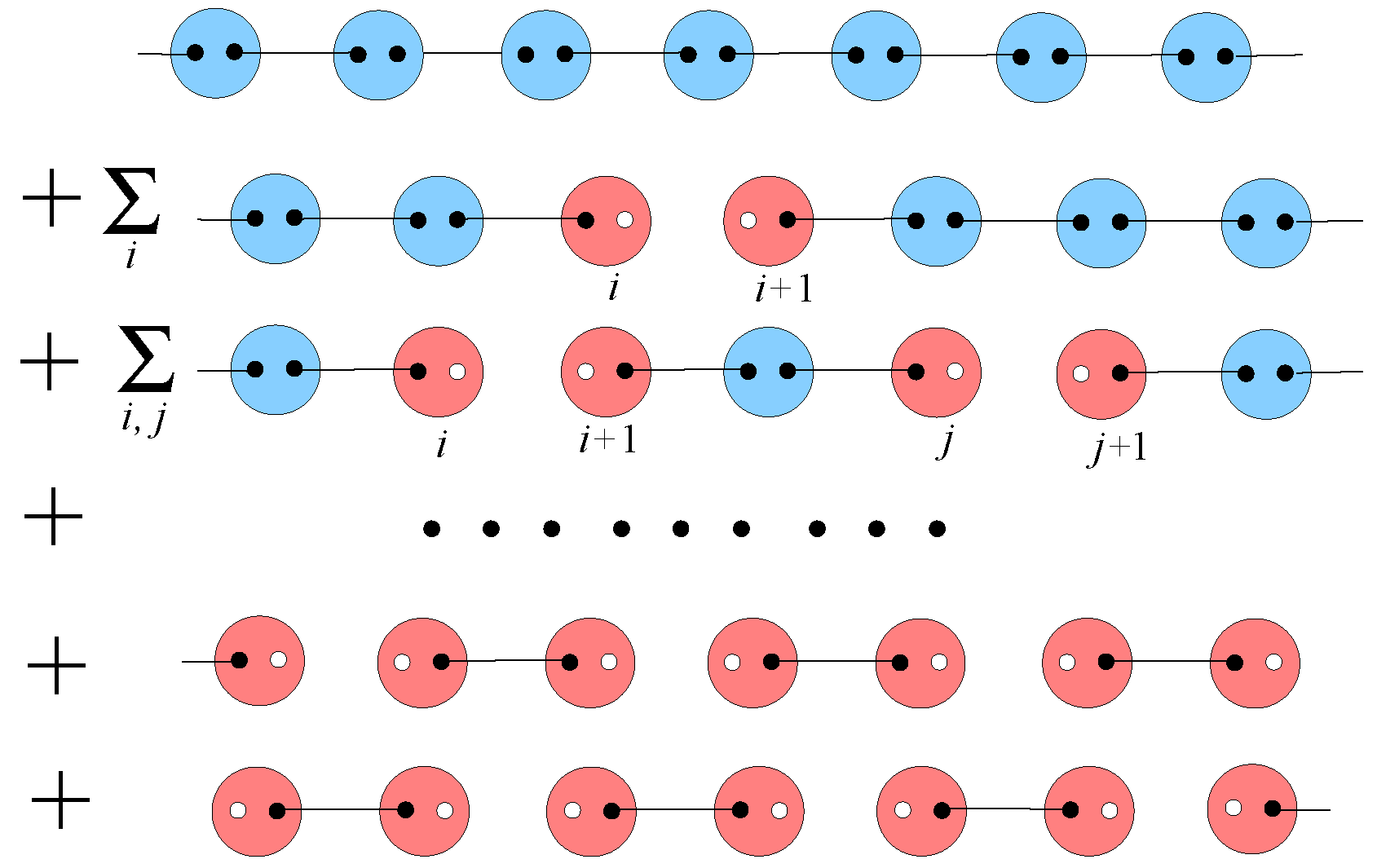
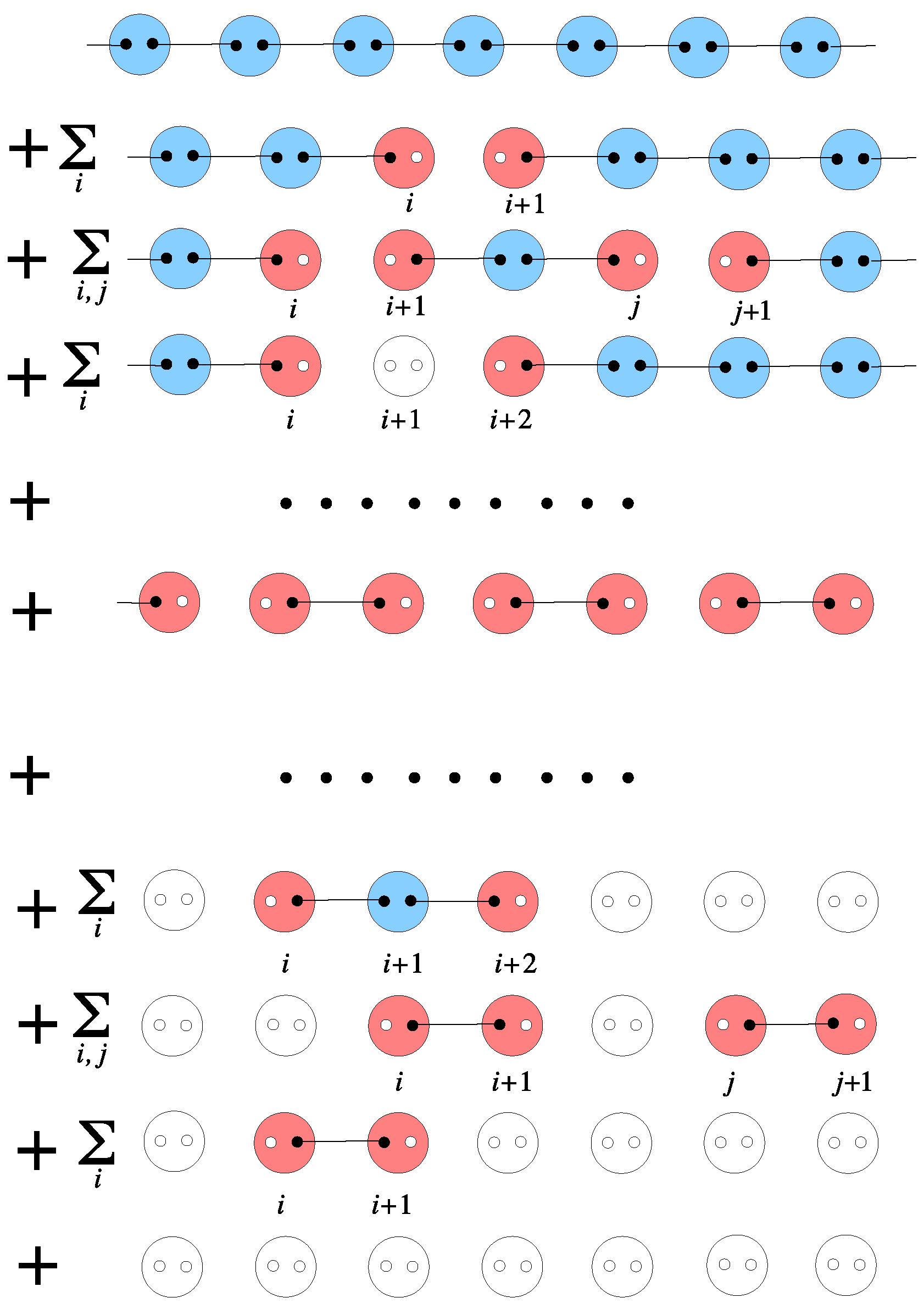
4.1. Construction of SVBS States
4.1.1.
| Schwinger operator | quantum number | Spin state |
|---|---|---|
| 1/2 | ||
| 0 |

4.1.2.
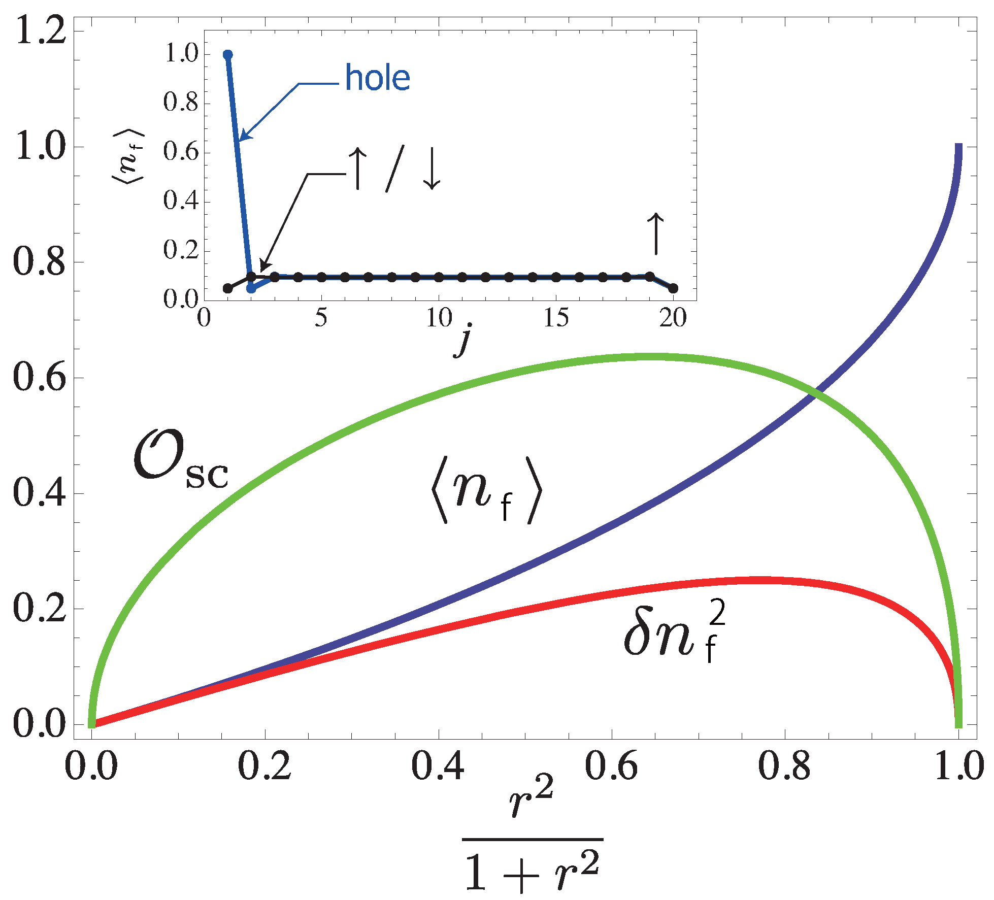
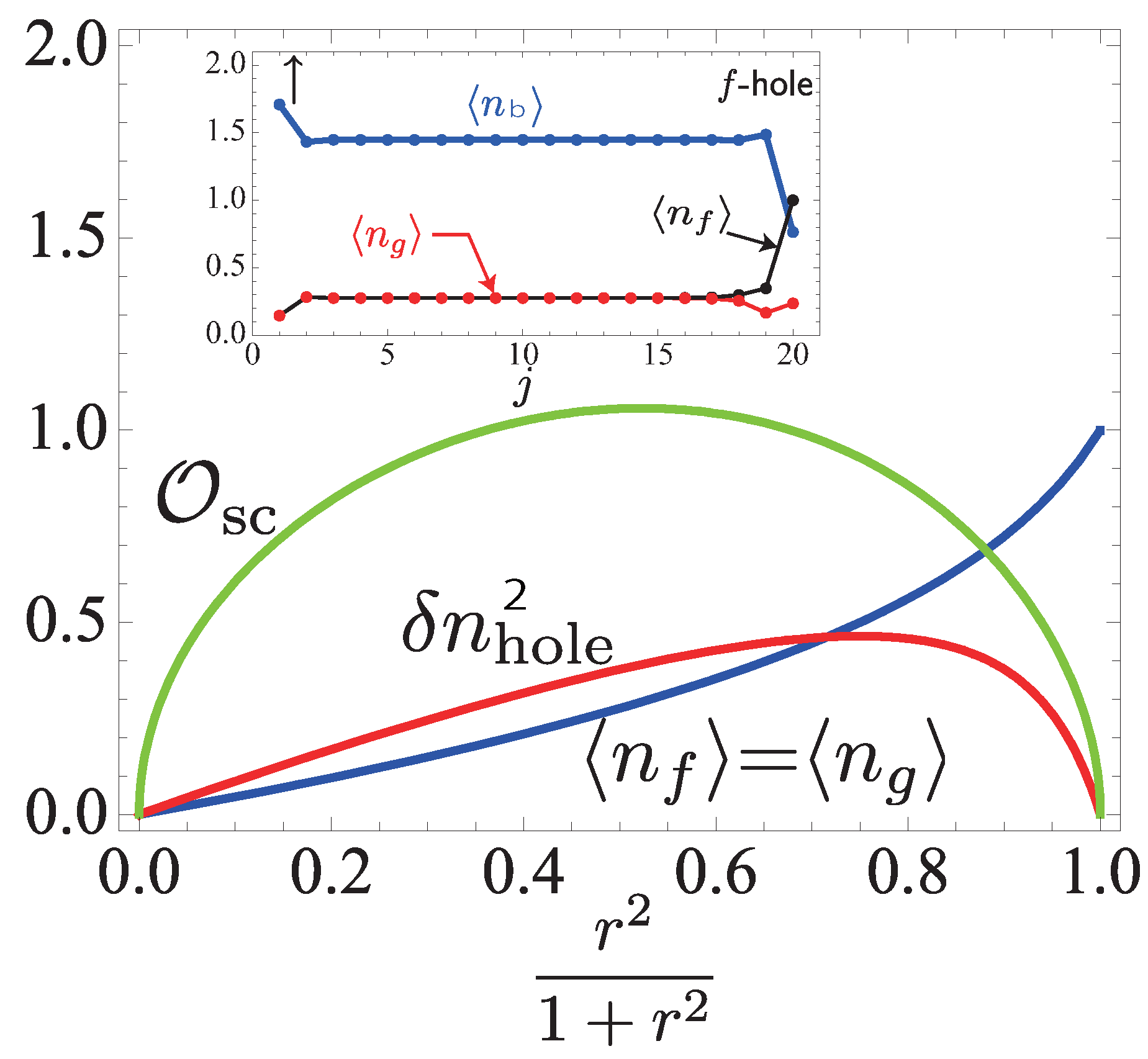
4.2. Superconducting Properties
4.2.1.
4.2.2.

4.3. Parent Hamiltonians
4.3.1.
4.3.2.
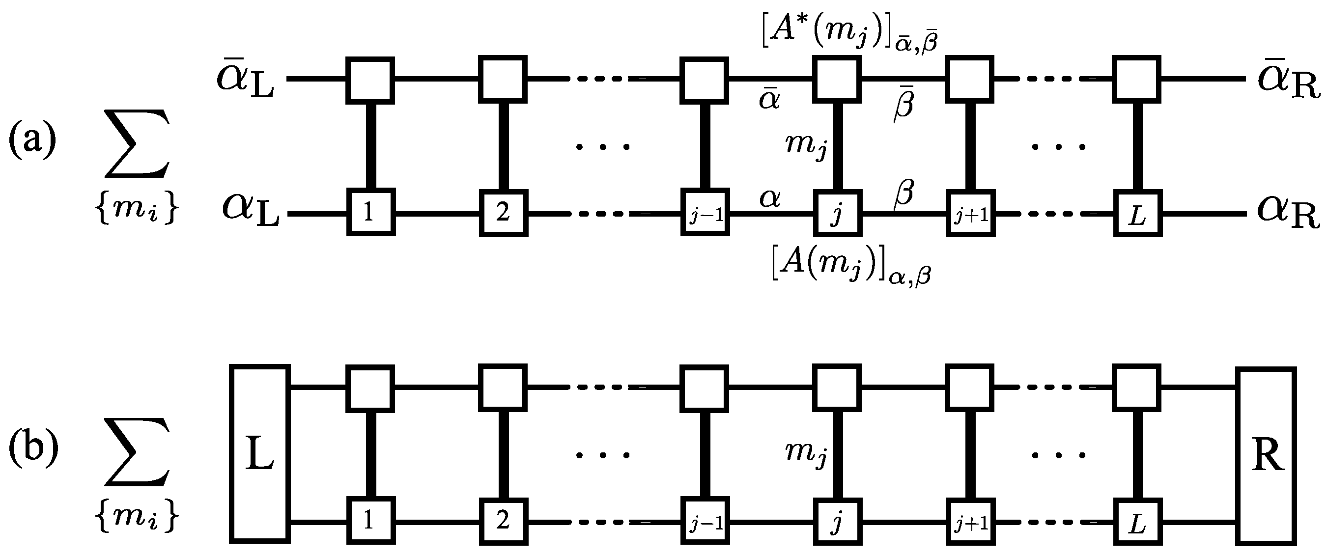
5. Supersymmetric Matrix Product State Formalism
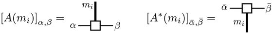
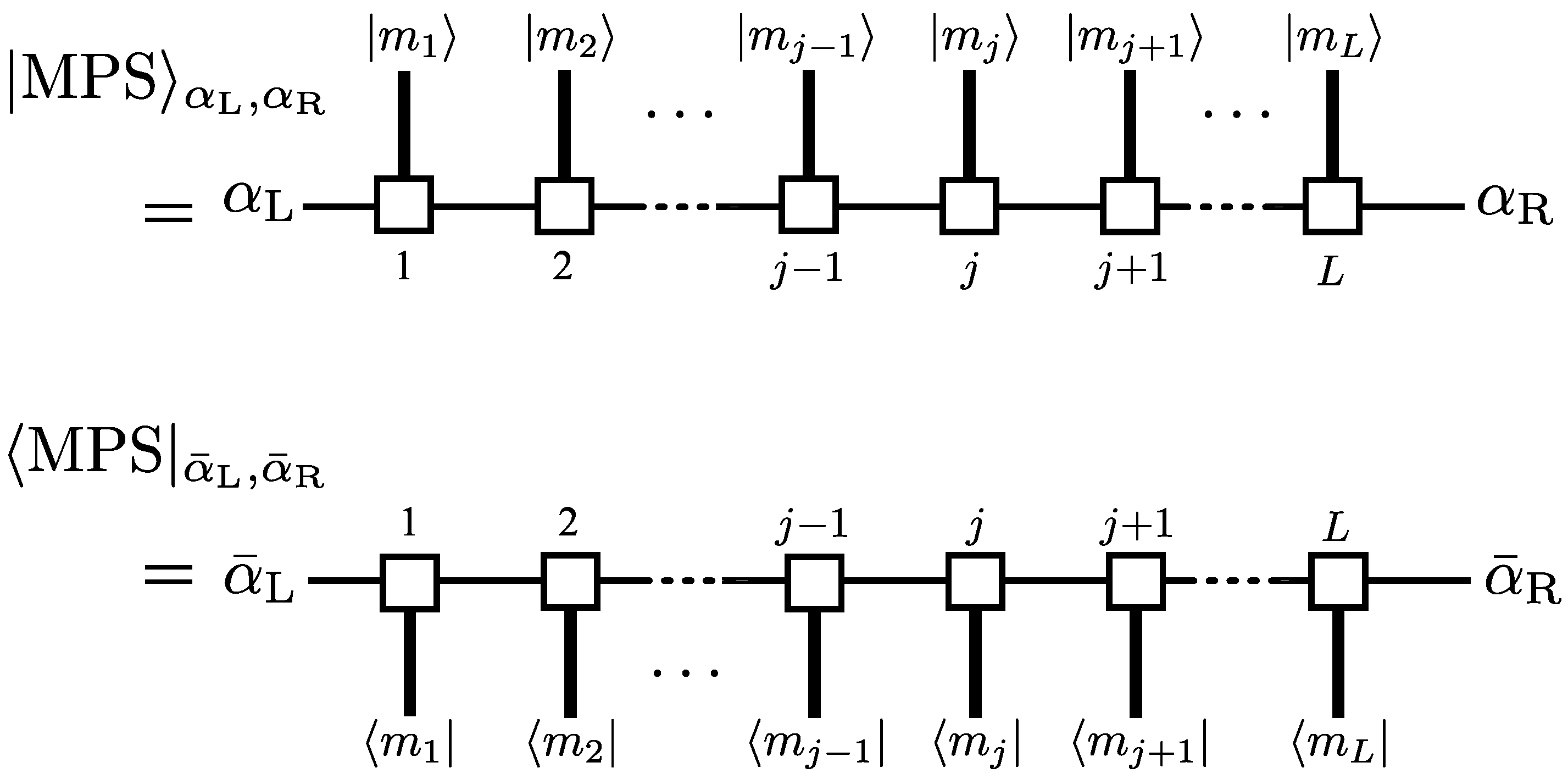
5.1. Bosonic Matrix Product State Formalism
5.2. Supermatrix-Product State (SMPS) Formalism and Edge States
5.2.1.

5.2.2.
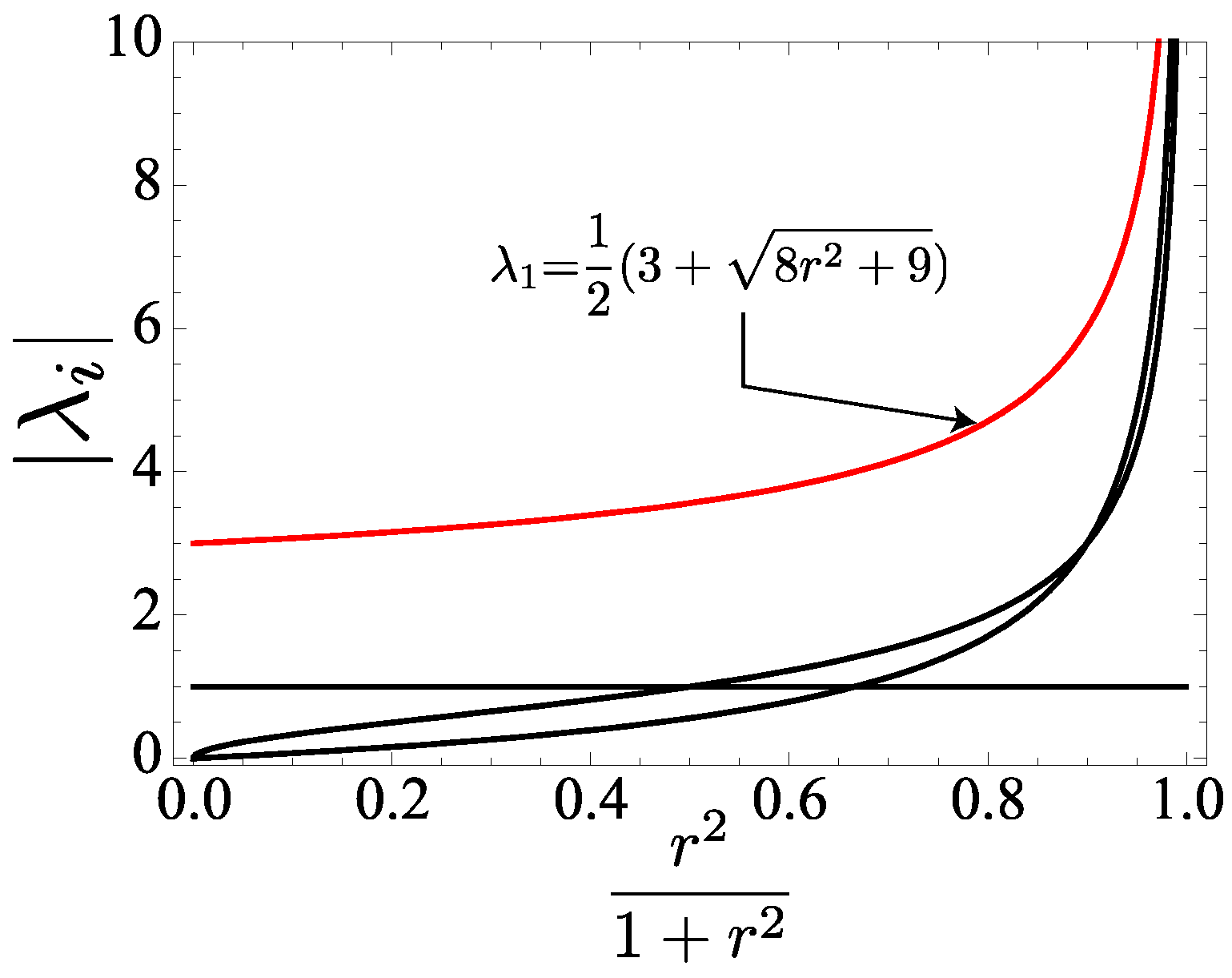
5.3. Excitations
5.3.1. Fixing Parent Hamiltonian
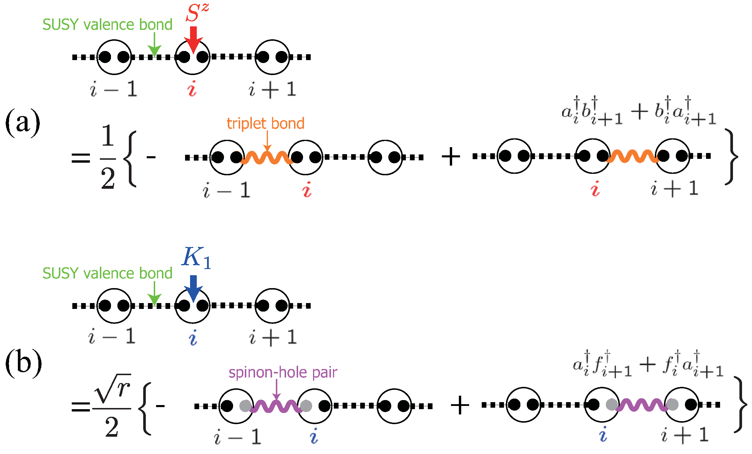
5.3.2. Crackion Excitation
- Spin excitation:Spin triplet excitation () created by bosonic operators
- Spinon-hole excitation:Spin doublet excitation () paired with a hole created by fermionic operators

5.3.3. Spin Excitation
5.3.4. Spinon-Hole Excitations


6. Topological Order
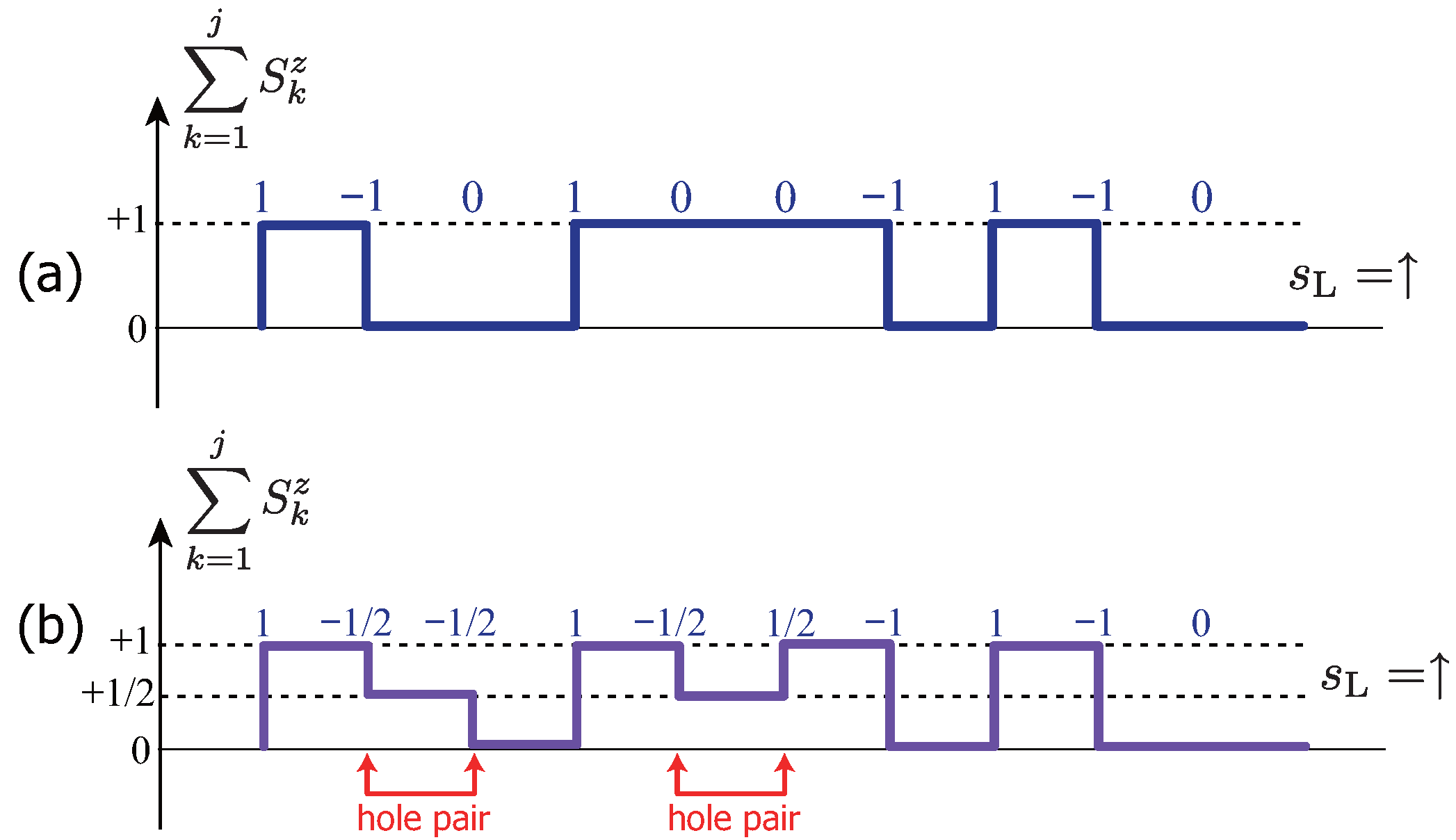
6.1. Hidden Antiferromagnetic Order and String Order Parameter
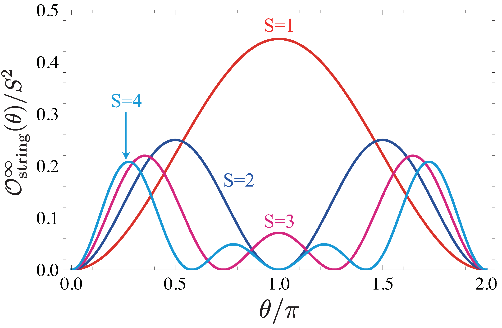
6.2. Generalized Hidden String Order in SVBS Chain
6.2.1.
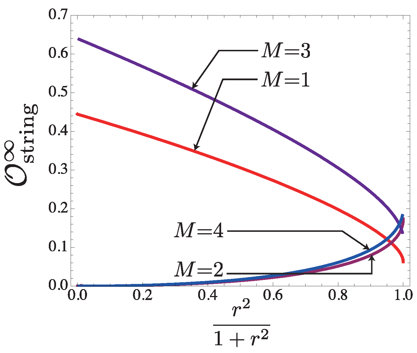
6.2.2.

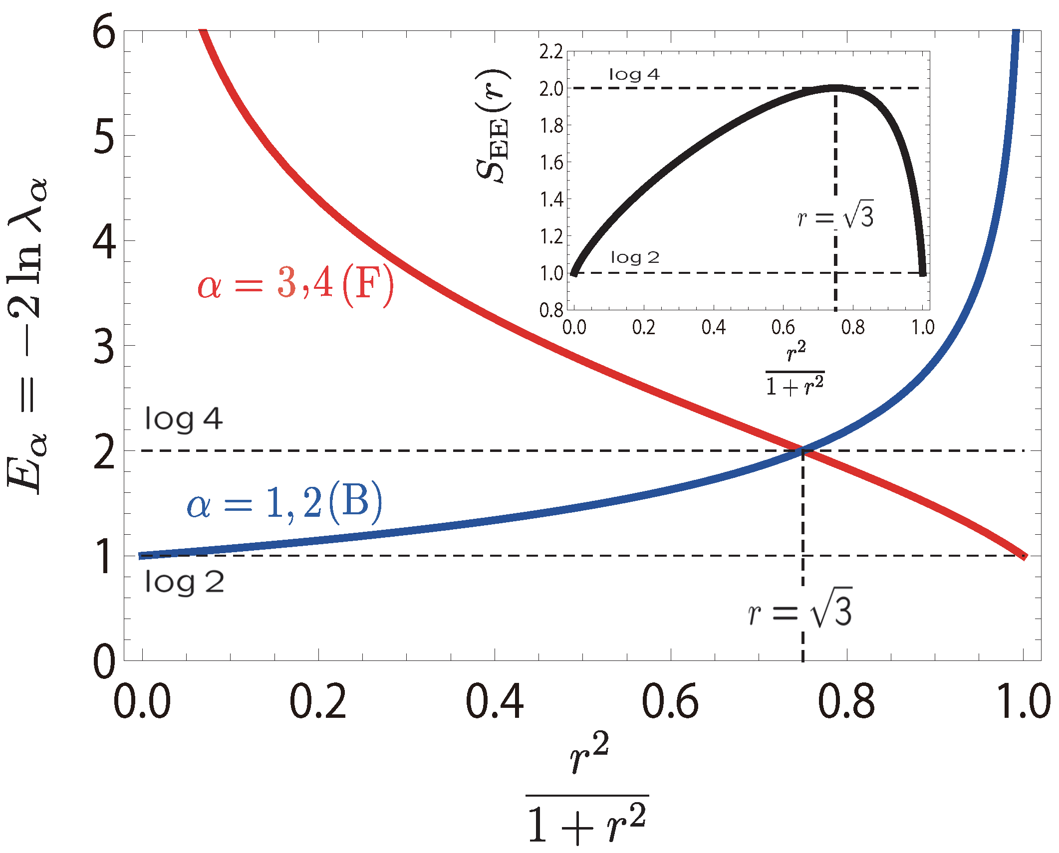
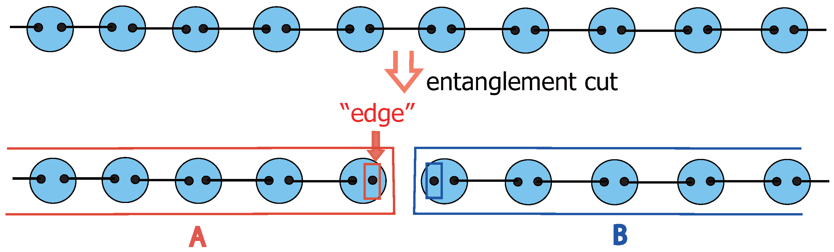
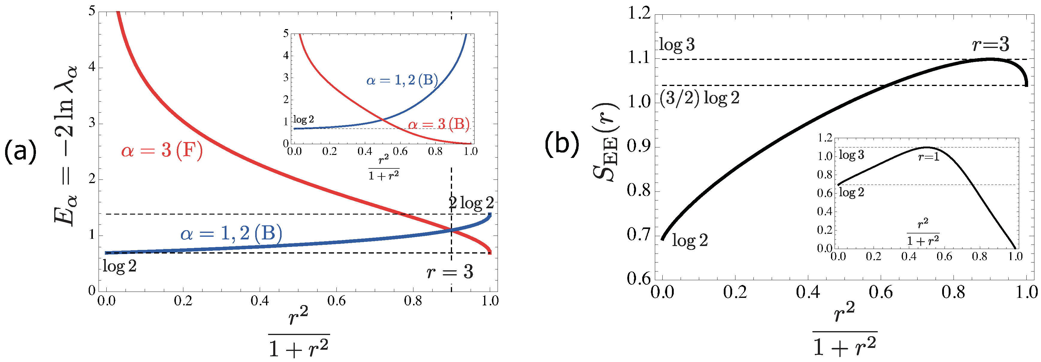
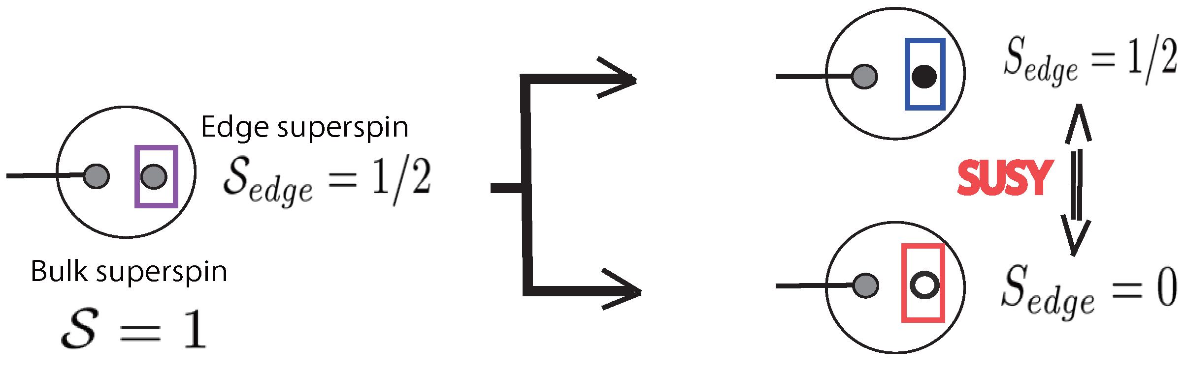
6.3. Entanglement Spectrum and Edge States
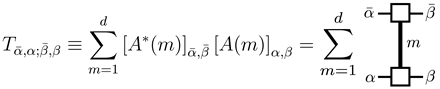
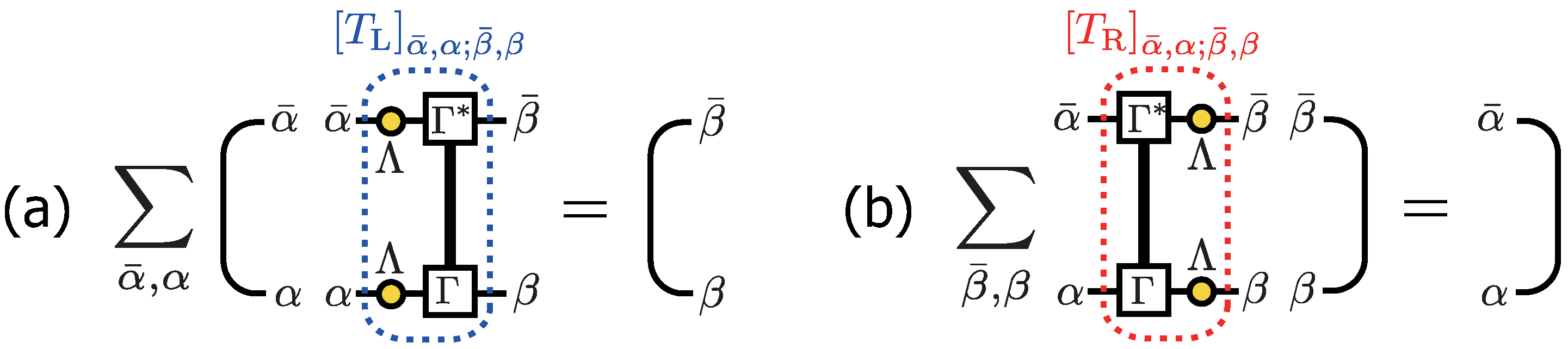
6.3.1. Schmidt Decomposition and Canonical Form of MPS


6.3.2.


6.3.3.

6.4. Supersymmetry-Protected Topological Order
6.4.1. Symmetry Operation and MPS
6.4.2. Case of SMPS
6.4.3. Inversion Symmetry
6.4.4. Time-Reversal Symmetry
6.4.5. Symmetry
6.4.6. String Order Parameters and Entanglement Spectrum


7. Higher Symmetric Generalizations
7.1. Fuzzy Four-Supersphere
7.2. SVBS States
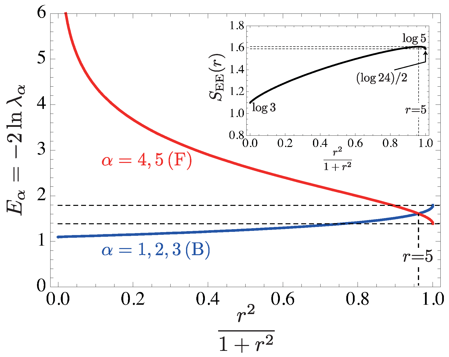
7.3. Entanglement Spectrum and Symmetry

8. Summary and Discussions
- Solvable parent Hamiltonian
- Gapped bulk and gapless edge excitations
- Generalized hidden order.
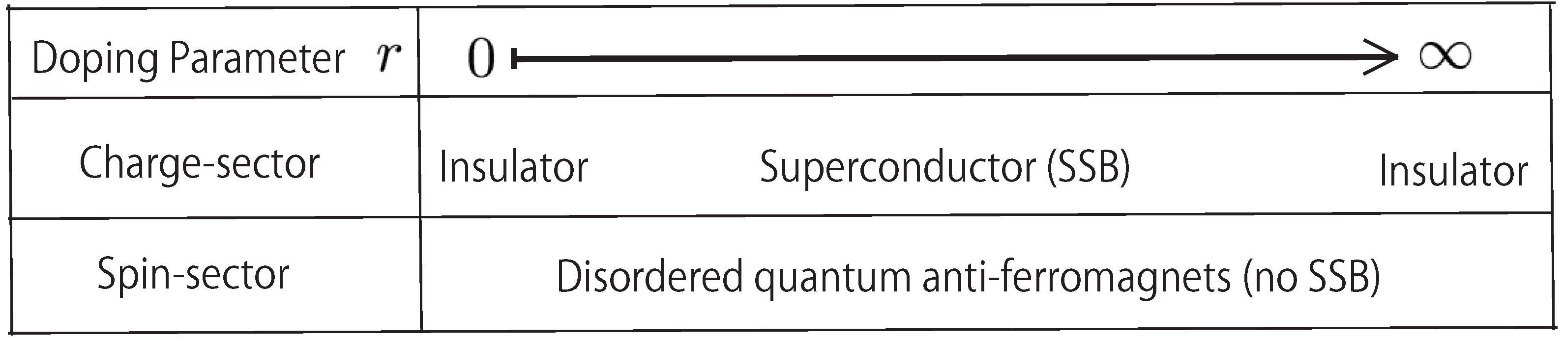
- In the charge sector, the SVBS states have the superconducting property (SSB).
- In spin sector, the SVBS states show a non-trivial topological order of QAFM (no SSB).
Acknowledgment
Appendix
A.
B. Fuzzy Four-Supersphere with Higher Supersymmetries
References and Notes
- Heisenberg, W. Mehrkörperproblem und resonanz in der quantenmechanik. Z. Phys. 1926, 38, 411–426. [Google Scholar] [CrossRef]
- Heisenberg, W. Zur theorie des ferromagnetismus. Z. Phys. 1928, 49, 619–636. [Google Scholar] [CrossRef]
- Bethe, H.A. Zur theorie der metalle i. eigenwerte und eigenfunktionen der linearen atomkette. Z. Phys. 1931, 71, 205–226. [Google Scholar] [CrossRef]
- Bardeen, J.; Cooper, L.N.; Schrieffer, J.R. Microscopic theory of superconductivity. Phys. Rev. 1957, 106, 162–164. [Google Scholar] [CrossRef]
- Laughlin, R.B. Anomalous quantum Hall effect: An incompressible quantum fluid with fractionally charged excitations. Phys. Rev. Lett. 1983, 50, 1395–1398. [Google Scholar] [CrossRef]
- Affleck, I.; Kennedy, T.; Lieb, E.; Tasaki, H. Rigorous results on valence-bond ground states in antiferromagnets. Phys. Rev. Lett. 1987, 59, 799–802. [Google Scholar] [CrossRef] [PubMed]
- Affleck, I.; Kennedy, T.; Lieb, E.; Tasaki, H. Valence bond ground states in isotropic quantum antiferromagnets. Commun. Math. Phys. 1988, 115, 477–528. [Google Scholar] [CrossRef]
- Arovas, D.P.; Hasebe, K.; Qi, X.-L.; Zhang, S.-C. Supersymmetric Valence Bond Solid States. Phys. Rev. 2009, B79, 224404:1–224404:20. [Google Scholar] [CrossRef]
- Hasebe, K.; Totsuka, K. Hidden order and dynamics in supersymmetric valence bond solid states–super-matrix product state formalism. Phys. Rev. 2011, B84, 104426:1–104426:19. [Google Scholar] [CrossRef]
- Hasebe, K.; Totsuka, K. Quantum entanglement and topological order in hole-doped valence bond solid states. Phys. Rev. B 2013, 87, 045115:1–045115:21. [Google Scholar] [CrossRef]
- Haldane, F.D.M. Continuum dynamics of the 1-D Heisenberg antiferromagnet: Identification with the O(3) nonlinear sigma model. Phys. Lett. A 1983, 93, 464–468. [Google Scholar] [CrossRef]
- Haldane, F.D.M. Nonlinear field theory of large-spin Heisenberg antiferromagnets: Semiclassically quantized solitons of the one-dimensional easy-axis Néel state. Phys. Rev. Lett. 1983, 50, 1153–1156. [Google Scholar] [CrossRef]
- Hagiwara, M.; Katsumata, K.; Affleck, I.; Halperin, B.I.; Renard, J.P. Observation of S = 1/2 degrees of freedom in an S = 1 linear-chain Heisenberg antiferromagnet. Phys. Rev. Lett. 1990, 65, 3181–3184. [Google Scholar] [CrossRef] [PubMed]
- Kennedy, T. Exact diagonalisations of open spin-1 chains. J. Phys. Condens. Matter 1990, 2, 5737–5745. [Google Scholar] [CrossRef]
- Qi, X.-L.; Zhang, S.-C. The quantum spin Hall effect and topological insulators. Phys. Today 2010, 63, 33–38. [Google Scholar] [CrossRef]
- Hasan, M.Z.; Kane, C.L. Topological insulators. Rev. Mod. Phys. 2010, 82, 3045–3067. [Google Scholar] [CrossRef]
- Qi, X.-L.; Zhang, S.-C. Topological insulators and superconductors. Rev. Mod. Phys. 2011, 83, 1057–1110. [Google Scholar] [CrossRef]
- den Nijs, M.; Rommelse, K. Preroughening transitions in crystal surfaces and valence-bond phases in quantum spin chains. Phys. Rev. B 1989, 40, 4709–4734. [Google Scholar] [CrossRef]
- Tasaki, H. Quantum liquid in antiferromagnetic chains: A stochastic geometric approach to the Haldane gap. Phys. Rev. Lett. 1991, 66, 798–801. [Google Scholar] [CrossRef] [PubMed]
- Fannes, M.; Nachtergaele, B.; Werner, R.F. Exact antiferromagnetic ground states of quantum spin chains. Europhys. Lett. 1989, 10, 633–637. [Google Scholar] [CrossRef]
- Fannes, M.; Nachtergaele, B.; Werner, R.F. Finitely correlated states on quantum spin chains. Commun. Math. Phys. 1992, 144, 443–490. [Google Scholar] [CrossRef]
- Klu¨mper, A.; Schadschneider, A.; Zittartz, J. Equivalence and solution of anisotropic spin-1 models and generalized t-J fermion models in one dimension. J. Phys. A Math. Gen. 1991, 24, L955–L959. [Google Scholar] [CrossRef]
- Klu¨mper, A.; Schadschneider, A.; Zittartz, J. Ground-state properties of a generalized VBS-model. Z. Phys. B Conds. Matter 1992, 87, 281–287. [Google Scholar] [CrossRef]
- Totsuka, K.; Suzuki, M. Matrix formalism for the VBS-type models and hidden order. J. Phys. Condens. Matter 1995, 7, 1639–1662. [Google Scholar] [CrossRef]
- Pérez-García, D.; Verstraete, F.; Wolf, M.M.; Cirac, J.I. Matrix product state representations. Quantum Inf. Comput. 2007, 7, 401–430. [Google Scholar]
- Nielsen, M.A.; Chuang, I.L. Quantum Computation and Quantum Information; Cambridge University Press: Cambridge, UK, 2000. [Google Scholar]
- Amico, L.; Fazio, R.; Osterloh, A.; Vedral, V. Entanglement in many-body systems. Rev. Mod. Phys. 2008, 80, 517–576. [Google Scholar] [CrossRef]
- Li, H.; Haldane, F.D.M. Entanglement spectrum as a generalization of entanglement entropy: Identification of topological order in non-abelian fractional quantum Hall effect states. Phys. Rev. Lett. 2008, 101, 010504:1–010504:4. [Google Scholar] [CrossRef]
- Hastings, M.B. An area law for one-dimensional quantum systems. J. Stat. Mech. Theory Exp. 2007, P08024:1–P08024:14. [Google Scholar] [CrossRef]
- White, S.R. Density matrix formulation for quantum renormalization groups. Phys. Rev. Lett. 1992, 69, 2863–2866. [Google Scholar] [CrossRef] [PubMed]
- Östlund, S.; Rommer, S. Thermodynamic limit of the density matrix renormalization for the spin-1 Heisenberg chain. Phys. Rev. Lett. 1995, 75, 3537–3540. [Google Scholar] [CrossRef] [PubMed]
- Verstraete, F.; Murg, V.; Cirac, J.I. Matrix product states, projected entangled pair states, and variational renormalization group methods for quantum spin systems. Adv. Phys. 2008, 57, 143–224. [Google Scholar] [CrossRef]
- Schollwöck, U. The density-matrix renormalization group in the age of matrix product states. Ann. Phys. 2011, 326, 96–192. [Google Scholar] [CrossRef]
- Dukelsky, J.; Martin-Delgado, M.A.; Nishino, T.; Sierra, G. Equivalence of the variational matrix product method and the density matrix renormalization group applied to spin chains. Europhys. Lett. 1998, 43, 457–462. [Google Scholar] [CrossRef]
- Roman, J.M.; Sierra, G.; Dukelsky, J.; Martin-Delgado, M.A. The matrix product approach to quantum spin ladders. J. Phys. A Math. Gen. 1998, 31, 9729–9759. [Google Scholar] [CrossRef]
- Fledderjohann, A.; Klu¨mper, A.; Mu¨tter, K.-H. Diagrammatics for SU(2) invariant matrix product states. J. Phys. A Math. Gen. 2011, 44, 475302:1–475302:18. [Google Scholar] [CrossRef]
- Auerbach, A. Interacting Electrons and Quantum Magnetism; Springer: Heidelberg, Germany, 1994. [Google Scholar]
- Verstraete, F.; Cirac, J.I. Matrix product states represent ground states faithfully. Phys. Rev. B 2006, 73, 094423:1–094423:8. [Google Scholar] [CrossRef]
- Hastings, M.B. Solving gapped Hamiltonians locally. Phys. Rev. B 2006, 73, 085115:1–085115:13. [Google Scholar] [CrossRef]
- Vidal, G. Efficient classical simulation of slightly entangled quantum computations. Phys. Rev. Lett. 2003, 91, 147902:1–147902:4. [Google Scholar] [CrossRef]
- Vidal, G. Efficient simulation of one-dimensional quantum many-body systems. Phys. Rev. Lett. 2004, 93, 040502:1–040502:4. [Google Scholar] [CrossRef]
- White, S.R.; Feiguin, A.E. Real-time evolution using the density matrix renormalization group. Phys. Rev. Lett. 2004, 93, 076401:1–076401:4. [Google Scholar] [CrossRef]
- Daley, A.J.; Kollath, C.; Schollwoöck, U.; Vidal, G. Time-dependent density-matrix renormalization-group using adaptive effective Hilbert spaces. J. Stat. Mech. Theory Exp. 2004, P04005:1–P04005:28. [Google Scholar] [CrossRef]
- Vidal, G. Classical simulation of infinite-size quantum lattice systems in one spatial dimension. Phys. Rev. Lett. 2007, 98, 070201:1–070201:4. [Google Scholar] [CrossRef]
- Orús, R.; Vidal, G. Infinite time-evolving block decimation algorithm beyond unitary evolution. Phys. Rev. B 2008, 78, 155117:1–155117:11. [Google Scholar] [CrossRef]
- Schadschneider, A.; Zittartz, J. Variational study of isotropic spin-1 chains. Ann. Phys. 1995, 4, 157–163. [Google Scholar] [CrossRef]
- Kolezhuk, A.; Mikeska, H.-J.; Yamamoto, S. Matrix-product-states approach to Heisenberg ferrimagnetic spin chains. Phys. Rev. B 1997, 55, R3336–R3339. [Google Scholar] [CrossRef]
- Weichselbaum, A.; Verstraete, F.; Schollwöck, U.; Cirac, J.I.; von Delft, J. Variational matrix-product-state approach to quantum impurity models. Phys. Rev. B 2009, 80, 165117:1–165117:7. [Google Scholar] [CrossRef]
- Porras, D.; Verstraete, F.; Cirac, J.I. Renormalization algorithm for the calculation of spectra of interacting quantum systems. Phys. Rev. B 2006, 73, 014410:1–014410:7. [Google Scholar] [CrossRef]
- Fan, H.; Korepin, V.; Roychowdhury, V. Entanglement in a valence-bond solid state. Phys. Rev. Lett. 2004, 93, 227203:1–227203:4. [Google Scholar] [CrossRef]
- Katsura, H.; Hirano, T.; Hatsugai, Y. Exact analysis of entanglement in gapped quantum spin chains. Phys. Rev. B 2007, 76, 012401:1–012401:4. [Google Scholar] [CrossRef]
- Katsura, H.; Hirano, T.; Korepin, V.E. Entanglement in an SU(n) valence-bond-solid state. J. Phys. A Math Theor. 2008, 41, 135304:1–135304:13. [Google Scholar] [CrossRef]
- Xu, Y.; Katsura, H.; Hirano, T.; Korepin, V.E. Entanglement and density matrix of a block of spins in AKLT model. J. Stat. Phys. 2008, 133, 347–377. [Google Scholar] [CrossRef]
- Niggemann, H.; Klu¨mper, A.; Zittartz, J. Quantum phase transition in spin-3/2 systems on the hexagonal lattice - optimum ground state approach. Z. Phys. B 1997, 104, 103–110. [Google Scholar] [CrossRef]
- Niggemann, H.; Klu¨mper, A.; Zittartz, J. Ground state phase diagram of a spin-2 antiferromagnet on the square lattice. Eur. Phys. J. B 2000, 13, 15–19. [Google Scholar] [CrossRef]
- Klümper, A.; Schadschneider, A.; Zittartz, J. Matrix product ground states for one-dimensional spin-1 quantum antiferromagnets. Eur. Phys. Lett. 1993, 24, 293–297. [Google Scholar] [CrossRef]
- Wolf, M.M.; Ortiz, G.; Verstraete, F.; Cirac, J.I. Quantum phase transitions in matrix product systems. Phys. Rev. Lett. 2006, 97, 110403:1–110403:4. [Google Scholar] [CrossRef]
- Vidal, G.; Latorre, J.I.; Rico, E.; Kitaev, A. Entanglement in quantum critical phenomena. Phys. Rev. Lett. 2003, 90, 227902:1–227902:4. [Google Scholar] [CrossRef]
- Calabrese, P.; Cardy, J. Entanglement entropy and quantum field theory. J. Stat. Mech. 2004, P06002:1–P06002:27. [Google Scholar] [CrossRef]
- Calabrese, P.; Cardy, J. Entanglement entropy and conformal field theory. J. Phys. A Math. Theor. 2009, 42, 504005:1–504005:36. [Google Scholar] [CrossRef]
- Chen, X.; Gu, Z.-C.; Wen, X.-G. Classification of gapped symmetric phases in one-dimensional spin systems. Phys. Rev. B 2011, 83, 035107:1–035107:19. [Google Scholar] [CrossRef]
- Chen, X.; Gu, Z.-C.; Wen, X.-G. Complete classification of one-dimensional gapped quantum phases in interacting spin systems. 2011; 84, 235128:1–235128:14. [Google Scholar]
- Gu, Z.-C.; Wen, X.-G. Tensor-entanglement-filtering renormalization approach and symmetry-protected topological order. Phys. Rev. B 2009, 80, 155131:1–155131:26. [Google Scholar] [CrossRef]
- Schuch, N.; Pérez-García, D.; Cirac, I. Classifying quantum phases using matrix product states and projected entangled pair states. Phys. Rev. B 2011, 84, 165139:1–165139:21. [Google Scholar] [CrossRef]
- Pollmann, F.; Turner, A.M.; Berg, E.; Oshikawa, M. Entanglement spectrum of a topological phase in one dimension. Phys. Rev. B 2010, 81, 064439:1–064439:10. [Google Scholar] [CrossRef]
- Pollmann, F.; Berg, E.; Turner, A.M.; Oshikawa, M. Symmetry protection of topological order in one-dimensional quantum spin systems. Phys. Rev. B 2012, 85, 075125:1–075125:9. [Google Scholar] [CrossRef]
- Turner, A.; Pollmann, F.; Berg, E. Topological phases of one-dimensional fermions: An entanglement point of view. Phys. Rev. B 2011, 83, 075102:1–075102:11. [Google Scholar] [CrossRef]
- Fidkowski, L.; Kitaev, A. Topological phases of fermions in one dimension. Phys. Rev. B 2011, 83, 075103:1–075103:13. [Google Scholar] [CrossRef]
- Duivenvoorden, K.; Quella, T. On topological phases of spin chains. Phys. Rev. B 2013, 87, 125145:1–125145:16. [Google Scholar] [CrossRef]
- Duivenvoorden, K.; Quella, T. A discriminating string order parameter for topological phases of gapped SU(N) spin chains. Phys. Rev. B 2012, 86, 235142:1–235142:13. [Google Scholar] [CrossRef]
- Zang, J.; Jiang, H.-C.; Weng, Z.-Y.; Zhang, S.-C. Topological quantum phase transition in an S = 2 spin chain. Phys. Rev. B 2010, 81, 224430:1–224430:6. [Google Scholar] [CrossRef]
- Zheng, D.; Zhang, G.-M.; Xiang, T.; Lee, D.-H. Continuous quantum phase transition between two topologically distinct valence bond solid states associated with the same spin value. Phys. Rev. B 2011, 83, 014409:1–014409:7. [Google Scholar] [CrossRef]
- Snyder, H.S. Quantized space-time. Phys. Rev. 1947, 71, 38–41. [Google Scholar] [CrossRef]
- Balachandran, A.P.; Qureshi, B.A. Noncommutative geometry: Fuzzy spaces, the groenewold-moyal plane. SIGMA 2006, 2, 094:1–094:9. [Google Scholar] [CrossRef]
- Arovas, D.P.; Auerbach, A.; Haldane, F.D.M. Extended Heisenberg models of antiferromagnetism: Analogies to the fractional quantum Hall effect. Phys. Rev. Lett. 1988, 60, 531–534. [Google Scholar] [CrossRef] [PubMed]
- Haldane, F.D.M. Fractional quantization of the Hall effect: A hierarchy of incompressible quantum fluid states. Phys. Rev. Lett. 1983, 51, 605–608. [Google Scholar] [CrossRef]
- For a review, see Hasebe, K. Hopf maps, lowest landau level, and fuzzy spheres. SIGMA 2010, 6, 071:1–071:42. [Google Scholar]
- Karabali, D.; Nair, V.P. Quantum Hall effect in higher dimensions, matrix models and fuzzy geometry. J. Phys. A 2006, 39, 12735–12764. [Google Scholar] [CrossRef]
- Zhang, S.-C.; Hu, J.-P. A four-dimensional generalization of the quantum Hall effect. Science 2001, 294, 823–828. [Google Scholar] [CrossRef] [PubMed]
- Bernevig, B.A.; Hu, J.-P.; Toumbas, N.; Zhang, S.-C. The eight dimensional quantum Hall effect and the octonions. Phys. Rev. Lett. 2003, 91, 236803:1–236803:4. [Google Scholar] [CrossRef]
- Hasebe, K.; Kimura, Y. Dimensional hierarchy in quantum Hall effects on fuzzy spheres. Phys. Lett. 2004, B602, 255–260. [Google Scholar] [CrossRef]
- Karabali, D.; Nair, V.P. Quantum Hall effect in higher dimensions. Nucl. Phys. 2002, B641, 533–546. [Google Scholar] [CrossRef]
- Bellucci, S.; Casteill, P.-Y.; Nersessian, A. Four-dimensional Hall mechanics as a particle on CP3. Phys. Lett. B 2003, 574, 121–128. [Google Scholar] [CrossRef]
- Geloun, J.B.; Govaerts, J.; Hounkonnou, M.N. A (p,q)-deformed Landau problem in a spherical harmonic well: Spectrum and noncommuting coordinates. Europhys. Lett. 2007, 80, 30001:1–37005:6. [Google Scholar] [CrossRef]
- Jellal, A. Quantum Hall effect on higher dimensional spaces. Nucl. Phys. B 2005, 725, 554–576. [Google Scholar] [CrossRef]
- Daoud, M.; Jellal, A. Quantum Hall effect on the flag manifold F2. Int. J. Mod. Phys. A 2008, 23, 3129–3154. [Google Scholar] [CrossRef]
- Hasebe, K. Hyperbolic supersymmetric quantum Hall effect. Phys. Rev. D 2008, 78, 125024:1–125024:13. [Google Scholar] [CrossRef]
- Hasebe, K. Split-quaternionic Hopf map, quantum Hall effect and twistor theory. Phys. Rev. D 2010, 81, 041702(R):1–041702(R):5. [Google Scholar] [CrossRef]
- Bellissard, J.; van Elst, A.; Schulz Baldes, H. The noncommutative geometry of the quantum Hall effect. J. Math. Phys. 1994, 35, 5373–5451. [Google Scholar] [CrossRef]
- Girvin, S.M.; Jach, T. Formalism for the quantum Hall effect: Hilbert space of analytic functions. Phys. Rev. B 1984, 29, 5617–5625. [Google Scholar] [CrossRef]
- Girvin, S.M.; MacDonald, A.H.; Platzman, P.M. Collective-excitation gap in the fractional quantum Hall effect. Phys. Rev. Lett. 1985, 54, 581–583. [Google Scholar] [CrossRef] [PubMed]
- Girvin, S.M.; MacDonald, A.H.; Platzman, P.M. Magneto-roton theory of collective excitations in the fractional quantum Hall effect. Phys. Rev. B 1986, 33, 2481–2494. [Google Scholar] [CrossRef]
- Ezawa, Z.F.; Tsitsishvili, G.; Hasebe, K. Noncommutative geometry, extended W(infty) algebra and grassmannian solitons in multicomponent quantum Hall systems. Phys. Rev. B 2003, 67, 125314:1–125314:16. [Google Scholar] [CrossRef]
- Berezin, F.A. General concept of quantization. Commun. Math. Phys. 1975, 40, 153–174. [Google Scholar] [CrossRef]
- Hoppe, J. Quantum Theory of a Massless Relativistic Surface and a Two-Dimensional Bound State Problem. Ph.D. Thesis, Massachusetts Institute of Technology, Cambridge, MA, USA, 1982. [Google Scholar]
- Madore, J. The fuzzy sphere. Class. Quant. Grav. 1992, 9, 69–87. [Google Scholar] [CrossRef]
- Grosse, H.; Klimcik, C.; Presnajder, P. On finite 4D quantum field theory in non-commutative geometry. Commun. Math. Phys. 1996, 180, 429–438. [Google Scholar] [CrossRef]
- Kabat, D.; Taylor, W. Spherical membranes in Matrix theory. Adv. Theor. Math. Phys. 1998, 2, 181–206. [Google Scholar]
- Ramgoolam, S. On spherical harmonics for fuzzy spheres in diverse dimensions. Nucl. Phys. B 2001, 610, 461–488. [Google Scholar] [CrossRef]
- Ho, P.-M.; Ramgoolam, S. Higher dimensional geometries from matrix brane constructions. Nucl. Phys. B 2002, 627, 266–288. [Google Scholar] [CrossRef]
- Kimura, Y. Noncommutative gauge theory on fuzzy four-sphere and matrix model. Nucl. Phys. B 2002, 637, 177–198. [Google Scholar] [CrossRef]
- Kimura, Y. On higher dimensional fuzzy spherical branes. Nucl. Phys. B 2003, 664, 512–530. [Google Scholar] [CrossRef]
- Azuma, T.; Bagnoud, M. Curved-space classical solutions of a massive supermatrix model. Nucl. Phys. B 2003, 651, 71–86. [Google Scholar] [CrossRef]
- Alexanian, G.; Balachandran, A.P.; Immirzi, G.; Ydri, B. Fuzzy CP2. J. Geom. Phys. 2002, 42, 28–53. [Google Scholar] [CrossRef]
- Balachandran, A.P.; Dolan, B.P.; Lee, J.; Martin, X.; O’Connor, D. Fuzzy complex projective spaces and their star-products. J. Geom. Phys. 2002, 43, 184–204. [Google Scholar] [CrossRef]
- Carow-Watamura, U.; Steinacker, H.; Watamura, S. Monopole bundles over fuzzy complex projective spaces. J. Geom. Phys. 2005, 54, 373–399. [Google Scholar] [CrossRef]
- Podles, P. Quantum spheres. Lett. Math. Phys. 1987, 14, 193–202. [Google Scholar] [CrossRef]
- Ho, P.-M.; Li, M. Large N expansion from fuzzy AdS2. Nucl. Phys. 2000, B590, 198–212. [Google Scholar] [CrossRef]
- Fakhri, H.; Imaanpur, A. Dirac operator on fuzzy AdS2. J. High Energy Phys. 2003, 0303, 003:1–003:16. [Google Scholar] [CrossRef]
- DeBellis, J.; Sa¨mann, Ch.; Szabo, R.J. Quantized nambu-poisson manifolds and n-lie algebras. J. Math. Phys. 2010, 51, 122303:1–122303:34. [Google Scholar] [CrossRef]
- Hasebe, K. Non-compact Hopf maps and fuzzy ultra-hyperboloids. Nucl. Phys. B 2012, 865, 148–199. [Google Scholar] [CrossRef]
- Tu, H.; Zhang, G.; Xiang, T. String order and hidden topological symmetry in the SO(2n + 1) symmetric matrix product states. J. Phys. A 2008, 41, 415201:1–415201:7. [Google Scholar] [CrossRef]
- Tu, H.; Zhang, G.; Xiang, T. Class of exactly solvable SO(n) symmetric spin chains with matrix product ground states. Phys. Rev. B 2008, 78, 094404:1–094404:10. [Google Scholar] [CrossRef]
- Tu, H.-H.; Zhang, G.-M.; Xiang, T.; Liu, Z.-X.; Ng, T.-K. Topologically distinct classes of valence bond solid states with their parent Hamiltonians. Phys. Rev. B 2009, 80, 014401:1–014401:11. [Google Scholar] [CrossRef]
- Greiter, M.; Rachel, S.; Schuricht, D. Exact results for SU(3) spin chains: Trimer states, valence bond solids, and their parent Hamiltonians. Phys. Rev. B 2007, 75, 060401(R):1–060401(R):4. [Google Scholar] [CrossRef]
- Greiter, M.; Rachel, S. Valence bond solids for SU(n) spin chains: Exact models, spinon confinement, and the Haldane gap. Phys. Rev. B 2007, 75, 184441:1–184441:25. [Google Scholar] [CrossRef]
- Arovas, D. Simplex solid states of SU(N) quantum antiferromagnets. Phys. Rev. B 2008, 77, 104404:1–104404:14. [Google Scholar]
- Rachel, S.; Thomale, R.; Führinger, M.; Schmitteckert, P.; Greiter, M. Spinon confinement and the Haldane gap in SU(n) spin chains. Phys. Rev. B 2009, 80, 180420(R):1–180420(R):4. [Google Scholar] [CrossRef]
- Schuricht, D.; Rachel, S. Valence bond solid states with symplectic symmetry. Phys. Rev. B 2008, 78, 014430:1–014430:9. [Google Scholar] [CrossRef]
- Rachel, S. Spin 3/2 dimer model. Europhys. Lett. 2009, 86, 37005:1–37005:6. [Google Scholar] [CrossRef]
- Totsuka, K.; Suzuki, M. Hidden symmetry breaking in a generalized valence-bond solid model. J. Phys. A Math. Gen. 1994, 27, 6443–6456. [Google Scholar] [CrossRef]
- Arita, C.; Motegi, K. Spin-spin correlation functions of the q-valence-bond-solid state of an integer spin model. J. Math. Phys. 2011, 52, 063303:1–063303:15. [Google Scholar] [CrossRef]
- Santos, R.A.; Paraan, F.N.C.; Korepin, V.E.; Klu¨mper, A. Entanglement spectra of q-deformed higher spin VBS states. J. Phys. A Math. Theor. 2012, 45, 175303:1–175303:14. [Google Scholar] [CrossRef]
- Grosse, H.; Klimcik, C.; Presnajder, P. Field theory on a supersymmetric lattice. Commun. Math. Phys. 1997, 185, 155–175. [Google Scholar] [CrossRef]
- Grosse, H.; Reiter, G. The fuzzy supersphere. J. Geom. Phys. 1998, 28, 349–383. [Google Scholar] [CrossRef]
- Landi, G. Projective modules of finite type over the supersphere S2,2. J. Geom. Phys. 2001, 37, 47–62. [Google Scholar] [CrossRef]
- Balachandran, A.P.; Kurkcuoglu, S.; Rojas, E. The star product on the fuzzy supersphere. J. High Energy Phys. 2002, 0207, 056:1–056:23. [Google Scholar] [CrossRef]
- Hasebe, K. Graded Hopf maps and fuzzy superspheres. Nucl. Phys. B 2011, 853, 777–827. [Google Scholar] [CrossRef]
- Hasebe, K.; Kimura, Y. Fuzzy supersphere and supermonopole. Nucl. Phys. 2005, 94, 94–114. [Google Scholar] [CrossRef]
- Hasebe, K. Supersymmetric quantum-Hall effect on a fuzzy supersphere. Phys. Rev. Lett. 2005, 94, 206802:1–206802:4. [Google Scholar] [CrossRef]
- Hasebe, K. Quantum Hall liquid on a noncommutative superplane. Phys. Rev. D 2005, 72, 105017:1–105017:9. [Google Scholar] [CrossRef]
- Hasebe, K. Supersymmetric Chern-Simons theory and supersymmetric quantum Hall liquid. Phys. Rev. D 2006, 74, 045026:1–045026:12. [Google Scholar] [CrossRef]
- Ivanov, E.; Mezincescu, L.; Townsend, P.K. A super-flag landau model. 2004. arXiv:hep-th/0404108. Avaliable online: http://arxiv.org/abs/hep-th/0404108 (accessed on 16 April 2004).
- Ivanov, E.; Mezincescu, L.; Townsend, P.K. Planar super-landau models. J. High Energy Phys. 2006. [Google Scholar] [CrossRef]
- Curtright, Th.; Ivanov, E.; Mezincescu, L.; Townsend, P.K. Planar super-landau models revisited. J. High Energy Phys. 2007, 0704, 020:1–020:24. [Google Scholar] [CrossRef]
- Beylin, A.; Curtright, Th.L.; Ivanov, E.; Mezincescu, L.; Townsend, P.K. Unitary spherical super-landau models. J. High Energy Phys. 2008, 0810, 069:1–069:47. [Google Scholar] [CrossRef]
- Beylin, A.; Curtright, Th.; Ivanov, E.; Mezincescu, L. Generalized N = 2 super landau models. J. High Energy Phys. 2010. arXiv:1003.0218. Avaliable online: http://arxiv.org/abs/1003.0218 (accessed on 28 February 2010). [Google Scholar]
- Bychkov, V.; Ivanov, E. N = 4 Supersymmetric landau models. Nucl. Phys. B 2012, 863, 33–64. [Google Scholar] [CrossRef]
- Goykhman, M.; Ivanov, E.; Sidorov, S. Super landau models on odd cosets. Phys. Rev. D 2013, 87, 025026:1–025026:18. [Google Scholar] [CrossRef]
- Ivanov, E.; Mezincescu, L.; Townsend, P.K. Fuzzy CP(n|m) as a quantum superspace. 2003. arXiv:hep-th/0311159. Avaliable online: http://arxiv.org/abs/hep-th/0311159 (accessed on 18 November 2003).
- Murray, S.; Saemann, C. Quantization of flag manifolds and their supersymmetric extensions. Adv. Theor. Math. Phys. 2008, 12, 641–710. [Google Scholar] [CrossRef]
- Lazaroiu, C.I.; McNamee, D.; Saemann, C. Generalized Berezin-Toeplitz quantization of Kaehler supermanifolds. J. High Energy Phys. 2009, 0905, 055:1–055:44. [Google Scholar]
- Johnson, C.V. D-brane primer. 2000. arXiv:hep-th/0007170. Avaliable online: http://arxiv.org/abs/hep-th/0007170 (accessed on 21 July 2000).
- Taylor, W. M(atrix) theory: Matrix quantum mechanics as a fundamental theory. Rev. Mod. Phys. 2001, 73, 419–462. [Google Scholar] [CrossRef]
- Szabo, R.J. D-branes in noncommutative field theory. 2005. arXiv:hep-th/0512054. Avaliable online: http://arxiv.org/abs/hep-th/0512054 (accessed on 5 December 2005).
- Myers, R.C. Dielectric-branes. J. High Energy Phys. 1999. [Google Scholar] [CrossRef]
- Klimcik, C. A nonperturbative regularization of the supersymmetric Schwinger model. Commun. Math. Phys. 1999, 206, 567–586. [Google Scholar]
- Klimcik, C. An extended fuzzy supersphere and twisted chiral superfields. Commun. Math. Phys. 1999, 206, 587–601. [Google Scholar]
- Iso, S.; Umetsu, H. Gauge theory on noncommutative supersphere from supermatrix model. Phys. Rev. D 2004, 69, 1050033:1–1050033:7. [Google Scholar] [CrossRef]
- Iso, S.; Umetsu, H. Note on gauge theory on fuzzy supersphere. Phys. Rev. D 2004, 69, 105014:1–105014:7. [Google Scholar] [CrossRef]
- Douglas, M.R.; Nekrasov, N.A. Noncommutative field theory. Rev. Mod. Phys. 2001, 73, 977–1029. [Google Scholar] [CrossRef]
- Azuma, T. Matrix models and the gravitational interaction. 2004. arXiv:hep-th/0401120. Avaliable online: http://arxiv.org/abs/hep-th/0401120 (accessed on 18 January 2004).
- Balachandran, A.P.; Kurkcuoglu, S.; Vaidya, S. Lectures on Fuzzy and Fuzzy SUSY Physics; World Scientific Publishers Co. Inc.: Hackensack, NJ, USA, 2007. [Google Scholar]
- Abe, Y.C. Construction of Fuzzy Spaces and Their Applications to Matrix Models. Ph.D. Thesis, City College of the CUNY, New York, NY, USA, December 2005. [Google Scholar]
- Aschieri, P.; Blohmann, C.; Dimitrijevic, M.; Meyer, F.; Schupp, P.; Wess, J. A gravity theory on noncommutative spaces. Class. Quant. Grav. 2005, 22, 3511–3532. [Google Scholar] [CrossRef]
- Calmet, X.; Kobakhidze, A. Noncommutative general relativity. Phys. Rev. D 2005, 72, 045010:1–045010:5. [Google Scholar] [CrossRef]
- Kurkcuoglu, S.; Saemann, C. Drinfeld twist and general relativity with fuzzy spaces. Class. Quant. Grav. 2007, 24, 291–312. [Google Scholar] [CrossRef]
- Taylor, W. Lectures on D-Branes, Gauge Theory and M(atrices); The ICTP Series in Theoretical Physics; Volume 14, Gava, E., Masiero, A., Narain, K.S., Randjbar-Daemi, S., Senjanovic, G., Smirnov, A., Shafi, Q., Eds.; World Scientific Publishers Co. Inc.: Hackensack, NJ, USA, 1998; p. 192. [Google Scholar]
- Azuma, T. Matrix models and the gravitational interaction. Ph.D. Thesis, Kyoto University, Kyoto, Japan, January 2004. [Google Scholar]
- Abe, Y. Construction of fuzzy spaces and their applications to matrix models. 2010. arXiv:1002.4937. Avaliable online: http://arxiv.org/abs/1002.4937 (accessed on 26 February 2010).
- Carow-Watamura, U.; Watamura, S. Chirality and dirac operator on noncommutative sphere. Commun. Math. Phys. 1997, 183, 365–382. [Google Scholar] [CrossRef]
- Schwinger, J. On Angular Momentum. In Quantum Theory of Angular Momentum; Biedenharn, L.C., van Dam, H., Eds.; Academic Press: New York, NY, USA, 1965; pp. 229–279. [Google Scholar]
- Grosse, H.; Klimcik, C.; Presnajder, P. Topologically nontrivial field configurations in noncommutative geometry. Commun. Math. Phys. 1996, 178, 507–526. [Google Scholar] [CrossRef]
- Verstraete, F.; Wolf, M.M.; Pérez-García, D.; Cirac, J.I. Criticality, the area law, and the computational power of projected entangled pair states. Phys. Rev. Lett. 2006, 96, 220601:1–220601:4. [Google Scholar] [CrossRef]
- Pérez-García, D.; Verstraete, F.; Ignacio Cirac, J.; Wolf, M.M. PEPS as unique ground states of local Hamiltonians. Quantum Inf. Comput. 2008, 8, 0650–0663. [Google Scholar]
- Girvin, S.; Arovas, D. Hidden topological order in integer quantum spin chains. Phys. Scr. T 1989, 27, 156–159. [Google Scholar] [CrossRef]
- Hatsugai, Y. String correlation of quantum antiferromagnetic spin chains with S = 1 and 2. J. Phys. Soc. Jpn. 1992, 61, 3856–3860. [Google Scholar] [CrossRef]
- Pais, A.; Rittenberg, V. Semisimple graded Lie algebras. J. Math. Phys. 1975, 16, 2062:1–2062:12. [Google Scholar] [CrossRef]
- Scheunert, M.; Nahm, W.; Rittenberg, V. Irreducible representations of the osp(2,1) and spl(2,1) graded Lie algebra. J. Math.Phys. 1977, 18, 155:1–155:8. [Google Scholar] [CrossRef]
- Marcu, M. The representations of spl(2,1)-an example of representations of basic superalgebras. J. Math. Phys. 1980, 21, 1277:1–1277:7. [Google Scholar] [CrossRef]
- Landi, G.; Marmo, G. Extensions of lie superalgebras and supersymmetric abelian gauge fields. Phys. Lett. B 1987, 193, 61–66. [Google Scholar] [CrossRef]
- Bartocci, C.; Bruzzo, U.; Landi, G. Chern-Simons forms on principal superfiber bundles. J. Math. Phys. 1990, 31, 45:1–45:10. [Google Scholar] [CrossRef]
- Frappat, L.; Sciarrino, A.; Sorba, P. Dictionary on Lie Algebras and Superalgebras; Academic Press: Waltham, MA, USA, 2000. [Google Scholar]
- Borsten, L.; Dahanayake, D.; Duff, M.J.; Rubens, W. Superqubits. Phys. Rev. D 2010, 81, 105023:1–105023:16. [Google Scholar] [CrossRef]
- Majumdar, C.; Ghosh, D. On next-nearest-neighbor interaction in linear chain. II. J. Math. Phys. 1969, 10, 1388–1399. [Google Scholar] [CrossRef]
- Majumdar, C. Antiferromagnetic model with known ground state. J. Phys. C 1970, 3, 911–916. [Google Scholar] [CrossRef]
- Anderson, P. The resonating valence bond state in La2CuO4 and superconductivity. Science 1987, 235, 1196–1198. [Google Scholar] [CrossRef] [PubMed]
- Rokhsar, D.S.; Kivelson, S.A. Superconductivity and the quantum hard-core dimer gas. Phys. Rev. Lett. 1988, 61, 2376–2379. [Google Scholar] [CrossRef] [PubMed]
- Moore, G.; Read, N. Nonabelions in the fractional quantum Hall effect. Nucl. Phys. B 1991, 360, 362–396. [Google Scholar] [CrossRef]
- Schrieffer, J.R. Theory of Superconductivity; Advanced Book Classics; Westview Press: New York, NY, USA, 1999. [Google Scholar]
- Knabe, S. Energy gaps and elementary excitations for certain VBS-quantum antiferromagnets. J. Stat. Phys. 1988, 52, 627–638. [Google Scholar] [CrossRef]
- Arovas, D.P. Two exact excited states for the S = 1 AKLT chain. Phys. Lett. A 1989, 137, 431–433. [Google Scholar] [CrossRef]
- Lieb, E.; Schultz, T.; Mattis, D. Two soluble models of an antiferromagnetic chain. Ann. Phys. (N.Y.) 1961, 16, 407–466. [Google Scholar] [CrossRef]
- Fáth, G.; Sólyom, J. Solitonic excitations in the Haldane phase of a S = 1 chain. J. Phys. Condens. Matter 1993, 5, 8983–8998. [Google Scholar] [CrossRef]
- Bijl, A. The lowest wave function of the symmetrical many particles system. Physica 1940, 7, 869–886. [Google Scholar] [CrossRef]
- Feynman, R.P. Atomic theory of the two-fluid model of liquid helium. Phys. Rev. 1954, 94, 262–277. [Google Scholar] [CrossRef]
- Xu, G.; Aeppli, G.; Bisher, M.E.; Broholm, C.; DiTusa, J.F.; Frost, C.D.; Ito, T.; Oka, K.; Paul, R.L.; Takagi, H.; Treacy, M.M.J. Holes in a quantum spin liquid. Science 2000, 289, 419–422. [Google Scholar] [CrossRef] [PubMed]
- Zhang, S.-C.; Arovas, D.P. Hole motion in an S = 1 chain. Phys. Rev. B 1989, 40, 2708–2711. [Google Scholar] [CrossRef]
- Penc, K.; Shiba, H. Propagating S = 1/2 particles in S = 1 Haldane-gap systems. Phys. Rev. B 1995, 52, R715–R718. [Google Scholar] [CrossRef]
- Kitaev, A.Y. Unpaired Majorana fermions in quantum wires. Phys.-Usp. 2001, 44, 131–136. [Google Scholar] [CrossRef]
- Kennedy, T.; Tasaki, H. Hidden Z2×Z2 symmetry breaking and the Haldane phase in the S = 1/2 quantum spin chain with bond alternation. Phys. Rev. B 1992, 45, 304–307. [Google Scholar] [CrossRef]
- Kennedy, T.; Tasaki, H. Hidden symmetry breaking and the Haldane phase S = 1 quantum spin chains. Commun. Math. Phys. 1992, 147, 431–484. [Google Scholar] [CrossRef]
- Oshikawa, M. Hidden Z2×Z2 symmetry in quantum spin chains with arbitrary integer spin. J. Phys. Condens. Matter 1992, 4, 7469–7488. [Google Scholar] [CrossRef]
- Schollwöck, U.; Jolicœur, T. Haldane gap and hidden order in the S = 2 antiferromagnetic quantum spin chain. Europhys. Lett. 1995, 30, 493–498. [Google Scholar] [CrossRef]
- Schollwöck, U.; Golinelli, O.; Jolicœur, T. S = 2 antiferromagnetic quantum spin chain. Phys. Rev. B 1996, 54, 4038–4051. [Google Scholar] [CrossRef]
- Anfuso, F.; Rosch, A. Fragility of string orders. Phys. Rev. B 2007, 76, 085124:1–085124:6. [Google Scholar] [CrossRef]
- Levin, M.; Wen, X.-G. Detecting topological order in a ground state wave function. Phys. Rev. Lett. 2006, 96, 110405:1–110405:4. [Google Scholar] [CrossRef]
- Kitaev, A.; Preskill, J. Topological entanglement entropy. Phys. Rev. Lett. 2006, 96, 110404:1–110404:4. [Google Scholar] [CrossRef]
- Pérez-García, D.; Wolf, M.M.; Sanz, M.; Verstraete, F.; Cirac, J.I. String order and symmetries in quantum spin lattices. Phys. Rev. Lett. 2008, 100, 167202:1–167202:4. [Google Scholar] [CrossRef]
- Sanz, M.; Wolf, M.M.; Pérez-García, D.; Cirac, J.I. Matrix product states: Symmetries and two-body Hamiltonians. Phys. Rev. A 2009, 79, 042308:1–042308:10. [Google Scholar] [CrossRef]
- Hatsugai, Y.; Kohmoto, M. Numerical study of the hidden antiferromagnetic order in the Haldane phase. Phys. Rev. B 1991, 44, 11789–11794. [Google Scholar] [CrossRef] [Green Version]
- Alcaraz, F.C.; Hatsugai, Y. String correlation functions in the anisotropic spin-1 Heisenberg chain. Phys. Rev. B 1992, 46, 13914–13918. [Google Scholar] [CrossRef] [Green Version]
- Yamamoto, S.; Miyashita, S. Thermodynamic properties of S = 1 antiferromagnetic Heisenberg chains as Haldane systems. Phys. Rev. B 1993, 48, 9528–9538. [Google Scholar] [CrossRef]
- Nishiyama, Y.; Totsuka, K.; Hatano, N.; Suzuki, M. Real-space renormalization-group analysisof the S = 2 antiferromagnetic Heisenberg chain. J. Phys. Soc. Jpn. 1995, 64, 414–422. [Google Scholar] [CrossRef]
- Haegeman, J.; Pérez-García, D.; Cirac, I.; Schuch, N. Order parameter for symmetry-protected phases in one dimension. Phys. Rev. Lett. 2012, 109, 050402:1–050402:5. [Google Scholar] [CrossRef]
- Pollmann, F.; Turner, A.M. Detection of symmetry-protected topological phases in one dimension. Phys. Rev. B 2012, 86, 125441:1–125441:13. [Google Scholar] [CrossRef]
- Zhang, S.-C. Exact microscopic wave function for a topological quantum membrane. Phys. Rev. Lett. 2003, 90, 196801:1–196801:4. [Google Scholar] [CrossRef]
- Tu, H.-H.; Orus, R. Intermediate Haldane phase in spin-2 quantum chains with uniaxial anisotropy. Phys. Rev. B 2011, 84, 140407(R):1–140407(R):4. [Google Scholar] [CrossRef]
- Yu, Y.; Yang, K. Supersymmetry and goldstino-like mode in bose-fermi mixtures. Phys. Rev. Lett. 2008, 100, 090404:1–090404:4. [Google Scholar] [CrossRef]
- Kaplan, D.B.; Sun, S. Spacetime as a topological insulator: Mechanism for the origin of the fermion generations. Phys. Rev. Lett. 2012, 108, 181807:1–181807:4. [Google Scholar] [CrossRef]
© 2013 by the authors; licensee MDPI, Basel, Switzerland. This article is an open access article distributed under the terms and conditions of the Creative Commons Attribution license (http://creativecommons.org/licenses/by/3.0/).
Share and Cite
Hasebe, K.; Totsuka, K. Topological Many-Body States in Quantum Antiferromagnets via Fuzzy Supergeometry. Symmetry 2013, 5, 119-214. https://doi.org/10.3390/sym5020119
Hasebe K, Totsuka K. Topological Many-Body States in Quantum Antiferromagnets via Fuzzy Supergeometry. Symmetry. 2013; 5(2):119-214. https://doi.org/10.3390/sym5020119
Chicago/Turabian StyleHasebe, Kazuki, and Keisuke Totsuka. 2013. "Topological Many-Body States in Quantum Antiferromagnets via Fuzzy Supergeometry" Symmetry 5, no. 2: 119-214. https://doi.org/10.3390/sym5020119