Non-Crystallographic Layer Lattice Restrictions in Order-Disorder (OD) Structures

Abstract

Symmetry operations of layers periodic in two dimensions restrict the geometry the lattice according to the five two-dimensional Bravais types of lattices. In order-disorder (OD) structures, the operations relating equivalent layers generally leave invariant only a sublattice of the layers. The thus resulting restrictions can be expressed in terms of linear relations of the ², ² and · scalar products of the lattice basis vectors with rational coefficients. To characterize OD families and to check their validity, these lattice restrictions are expressed in the bases of different layers and combined. For a more familiar notation, they can be expressed in terms of the lattice parameters a, b and γ. Alternatively, the description of the lattice restrictions may be simplified by using centered lattices. The representation of the lattice restrictions in terms of scalar products is dependent on the chosen basis. A basis-independent classification of the lattice restrictions is outlined.

1. Introduction

Already in the early days of structure characterization by diffraction methods, it had been observed that many solid compounds do not a feature long-range order despite being built according to strict and unambiguous chemical rules. One of these systems, the mineral, wollastonite (CaSiO₃) [1], and the isotypic inorganic compounds, Madrell’s salt (NaPO₃) and NaAsO₃ [2], sparked the development of the order-disorder (OD) theory [3]. The OD theory can be considered as the crystallographic theory of local symmetry and has, since its inception, been developed into a versatile theory for the explanation and description of polytypism, diffuse scattering, non-crystallographic absences, twinning and as a means to classify structures by “symmetry principles” [4]. The fruitful application of OD theory to all major classes of compounds—from minerals to biological macro-molecules [5]—demonstrates the universality of the underlying concepts. A concise introduction to OD theory was given by Ferraris et al. [6].

OD theory is based on the geometric (and as a consequence, energetic) equivalence of pairs of adjacent layers, which is expressed by the vicinity condition (VC) [7]. Slightly varying wordings of the VC have been given [7–11]. Usually, it is stated as three propositions:

• (VCα) OD structures are composed of a finite number of kinds of layers with two-dimensional lattices;

• (VCβ) The intersection of the lattices of all layers of an OD structure is a two-dimensional lattice;

• (VCγ) Equivalent sides (layers in which both sides are not equivalent, i.e., not related by symmetry, can adopt one of 17 layer group types, which correspond to the 17 plane group types. These layer groups and layers are said to be polar) of equivalent layers are faced by adjacent layers in such a way that the thus formed pairs of layers are equivalent.

Structures that fulfill the VC and that are not necessarily periodic in three dimensions are called proper OD structures, as opposed to fully-ordered structures [8]. The infinite number of stacking possibilities (polytypes) arising from a proper OD structure are said to belong to the same OD family. The local symmetry of a polytype is described by a groupoid [10], a generalization of the group concept. By abstracting from metric parameters, these groupoids are classified into OD groupoid families, which take the role of space group types in classical crystallography. Two alternative versions of VCβ have been proposed, leading to a stricter and a broader VC (VCα and VCγ are independent of VCβ and remain unchanged): The stricter VCβ′ [9,10] reads as:

• (VCβ′) All layers of an OD structure possess the same lattice.

and, on the other hand, the broader VCβ″ [10] as:

• (VCβ″) The intersection of the lattices of two adjacent layers of an OD structure is a two-dimensional lattice.

VCβ″ differs subtly from VCβ in that, whereas every given pair of layers possesses a common two-dimensional lattice, there can be polytypes in which these common lattices become more sparse with the increasing distance of the layers, and therefore, the whole polytype does not feature two-dimensional periodicity parallel to the layer planes. All polytypes of OD structures fulfilling VCβ, on the other hand, possess a common two-dimensional lattice parallel to the layer planes. As a consequence, OD structures in which layers are related by operations with a non-crystallographic rotation angle fulfill VCβ″, but not VCβ.

Most documented OD structures fulfill the strict and, from a theoretical point of view, less demanding VCβ′. Therefore, most work on OD theory, so far, like the derivation of the 400 OD groupoid families [12], is based on VCβ′. Moreover, a notation based on Hermann–Mauguin symbols for the designation of OD groupoid families has only been developed for families fulfilling VCβ′ [8,13]. Nevertheless, during our structural investigations, we have encountered polytypic structures where the inequality of the lattices of adjacent layers is the decisive factor giving rise to the OD character (e.g., KOH·2H₂O [14] and K₂HAsO₄ · 2.5H₂O [15]). Therefore, a complete OD theory must consider the more general VCβ and VCβ″.

The existence of certain symmetry operations of a layer imposes a minimum Bravais class of the layer lattice (the symmetry of the lattice can also accidentally belong to a higher-symmetry Bravais class [16]) and, therefore, restricts the geometry of the lattice. In OD structures, the layer lattices can additionally be restricted by operations relating distinct layers or by the combination (i.e., intersection) of the lattice restrictions of distinct layers. For the special case VCβ′, these restrictions correspond to those of the Bravais types of lattices, as will be recapitulated in Section 2.3. In OD structures fulfilling VCβ or VCβ″, but not the more strict VCβ′, the operations relating equivalent layers generally leave invariant only a sublattice of the layers. In this case, they lead to non-crystallographic layer lattice restrictions, which can be expressed as linear relationships of the scalar products of the primitive lattice basis vectors, as will be discussed in Section 2.4.

This representation has proven to be a useful computational device for the automated analysis of OD structures (like the derivation of stacking possibilities [17], polytypes with a maximum degree of order [18,19], family (superposition) structures [7], etc.). For this purpose, the lattice restrictions have to be transformed into different bases (Section 2.5) and combined (Section 2.6). A more familiar representation in terms of the lattice parameters a, b and γ will be developed in Section 2.7. An alternative, and perhaps more convenient, description may be obtained by using centered lattices, as shown in Section 2.9. The representation of lattice restrictions by scalar products is dependent on the chosen basis. A basis-independent classification will be outlined in Section 2.11. Finally, examples are given in Section 2.12, and the discussed relations are derived in the Appendix.

2. Results and Discussion

2.1. Notations and Conventions

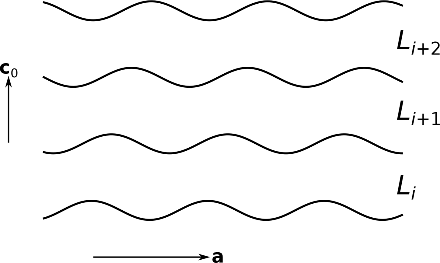
A layer is a connected, two-dimensionally periodic subspace of the three-dimensional Euclidean space E³ with continuously finite and non-zero thickness. Every point of an OD structure can be assigned to either a layer or the interface between two layers, which need not be planar (Figure 1). Thus, every layer is connected to exactly two neighbors. For simplicity, in the following text, all layers are normal to [001]. Layers are said to be equivalent or of the same kind if they are congruent or enantiomorphous [8], i.e., related by an isometry. When pairs of (not necessarily adjacent or equivalent) layers are considered, they will be called L_i and L_j, and the corresponding lattice basis vectors are (a_i, b_i) and (a_j, b_j). Subscripts are omitted if only one layer is examined. The lattice parameters of the layer L_i will be written as a_i = |a_i|, b_i = |b_i| and γ_i = a_i ∧ b_i. The notation a ∧ b designates (depending on the context) the measure of the angle between a and b or the angle itself (the origin being the vertex of the angle). Scalar products of vectors are indicated by a dot: a · b = |a||b| cos(a ∧ b), matrix multiplication by juxtaposition. For brevity, a · a = |a|² is shortened to a². The metric tensor of layer L_i is:

$${\mathbf{G}}_i=\left(\begin{array}{cc}{\mathbf{a}}_i^2& {\mathbf{a}}_i\cdot {\mathbf{b}}_i\\ {\mathbf{a}}_i\cdot {\mathbf{b}}_i& {\mathbf{b}}_i^2\end{array}\right)$$

(1)

Since the position of the different layers relative to one another is of no concern for the following discussion, layer lattices are regarded as vector lattices or translation groups. Thus, the lattice of layer L_i is 𝔏_i = {na_i + mb_i|n, m ∈ ℤ}. Accordingly, if 𝔏_j ⊂ 𝔏_i, 𝔏_j is said to be a strict sublattice of 𝔏_i, and 𝔏_i is considered as the larger lattice of the two, despite defining a smaller unit cell. Lattice vectors are designated by u; arbitrary directions are given as ua + vb. Rotation angles are denominated by ψ. The linear part of isometries of E³ (motions) is represented by the matrix M ; matrices of affine transformations operating on lattice basis vectors are written as P. I₂ is the 2 × 2 identity matrix. The 2 × 3 matrix A and the 3 × 1 column vectors V and U are used to describe the linear relationships of the scalar products a², b² and a·b. Q and R are 3×3 transformation matrices operating on V and U. o is the column vector of zero coefficients. The “×” symbol will be used in analogy to the cross-product of two coordinate vectors with respect to an orthonormal coordinate system:

$$\left(\begin{array}{c}x\\ y\\ z\end{array}\right)\times \left(\begin{array}{c}x\prime \\ y\prime \\ z\prime \end{array}\right)=\left(\begin{array}{c}yz\prime -zy\prime \\ zx\prime -xz\prime \\ xy\prime -yx\prime \end{array}\right)$$

(2)

λ and l are real numbers.

2.2. Partial Operations

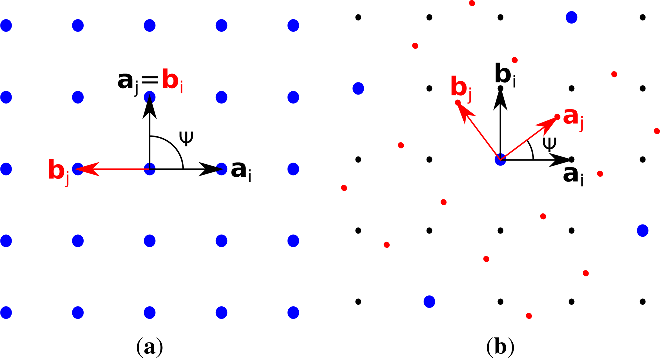
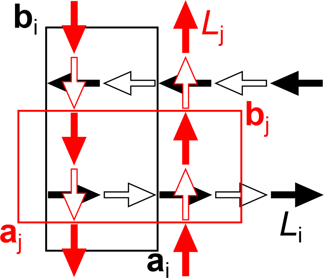
The operations relating equivalent layers are called partial operations (POs) [8] to highlight that they are not necessarily valid for the whole structure. A PO transforming L_i into L_j is called σ-PO if i ≠ j or λ-PO if i = j [8]. Expressed in the coordinate system of L_i, the linear part of a PO has the form:

$$\mathit{M}=\left(\begin{array}{ccc}{m}_{11}& m_{12}& 0\\ m_{21}& m_{22}& 0\\ 0& 0& \pm 1\end{array}\right)$$

(3)

In the context of layer lattice restrictions, only the action of the operation on the lattice basis vectors is relevant:

$$\left({\mathbf{a}}_j,{\mathbf{b}}_j\right)=\left({\mathbf{a}}_i,{\mathbf{b}}_i\right)\left(\begin{array}{cc}{p}_{11}& p_{12}\\ p_{21}& p_{22}\end{array}\right)=\left({\mathbf{a}}_i,{\mathbf{b}}_i\right)\mathit{P}$$

(4)

with p_ij = m_ij. Thus, the following discussion will be based on these two-dimensional lattice transformations, which correspond to the point group operations in two dimensions that map the origin onto itself, viz., rotations around the origin (including the identity) and mirror operations at lines passing through the origin. Since, according to VCβ (or VCβ″), the common sublattice of adjacent layers is a two-dimensional lattice, all elements p_ij ∈ ℚ [20] and, henceforth, only rational P are considered. In the special case of VCβ′, P is integral. Since POs are isometries, det(P) = ±1. Since two-dimensional lattices are symmetric by a two-fold rotation, mirroring at a line and the perpendicular line, as well as rotation by ψ and ψ + π are equivalent lattice transformations (i.e., both transform a given lattice into two identical lattices). Thus, P and −P represent equivalent lattice transformations. An overview of all kinds of σ-POs and the corresponding lattice transformations is compiled in

Table 1. Kinds of σ-partial operations (POs) and the corresponding two-dimensional lattice transformations. Rotations by ψ and ψ + π represent equivalent lattice transformations. The identity operation and rotations by ψ = π are listed separately from other rotations, since they impose different lattice restrictions, as will be shown below.

σ-PO	Type and orientation of element	det(M)	Lattice transformation	det(P)
rotation or screw by ψ = π	axis parallel to layer plane	1	} mirroring	−1
glide	plane normal to layer plane	−1
translation	–	1	} identity or rotation by π	}1
glide or mirroring	plane parallel to layer plane	−1
inversion	–	−1
screw by ψ = π	axis normal to layer plane	1
screw by ψ ≠ π	axis normal to layer plane	1	} rotation by ψ or ψ + π
rotoinversion by ψ ≠ 0, π	axis normal to layer plane	−1

Note: With the non-zero translational component normal to layer plane.

.

2.3. Layer Lattice Restrictions in the Case of Layer Groups and VCβ′

The necessity to restrict the geometry of lattices was recognized when deriving the symmetry groups of periodic objects in Euclidean space, viz., the crystallographic frieze, rod, plane, layer and space groups. Indeed, the symmetry operations of a periodic object may not be compatible with every lattice, resulting in the assignment of symmetry groups to Bravais types of lattices (usually shortened to “Bravais lattices”, but spelled out here to emphasize that it is a set of an infinity of lattices; the resulting classes of symmetry groups are called Bravais flocks) [16]. Note that the lattice may also accidentally be of a higher symmetry than is imposed by the group (e.g., an orthorhombic layer with a square lattice). There are five Bravais types of lattices in two dimensions [21], listed in

Table 2. The five Bravais types of lattices in two dimensions, the corresponding lattice system and the restrictions of the geometry expressed in the lattice parameters a, b and γ and in the scalar products of the basis vectors. The primitive bases are chosen according to [21].

Bravais type of lattices	Lattice system	Lattice restriction in standard primitive setting		Free parameters
		Lattice parameters	Basis vectors
mp	oblique	–	–	3
op	rectangular	$\gamma =\frac{\pi }{2}$	a · b = 0	2
oc	rectangular	a = b	a2 = b2	2
tp	square	a = b, $\gamma =\frac{\pi }{2}$	a2 = b2, a · b = 0	1
hp	hexagonal	a = b, $\gamma =\frac{2\pi }{3}$	a2 = b2, $\mathbf{a}\cdot \mathbf{b}=-\frac{{\mathbf{a}}^2}{2}$	1

with the corresponding restriction of the lattice geometry in the standard primitive setting.

In the context of OD theory, not only layer symmetry operations (λ-POs), but also σ-POs restrict the layer lattice. If all layers possess the same lattice (i.e., VCβ′ holds), the linear part of all (λ- and σ-) POs must map this two-dimensional lattice onto itself. Thus, all polytypes of an OD family that fulfills VCβ′ share the same common two-dimensional lattice, and the OD family can be assigned to one of the five two-dimensional Bravais types of lattices and, as consequence, to one of the four two-dimensional lattice systems although in two dimensions, the classifications into lattice and crystal systems are identical, the notion of lattice system is used here, since in three (or more) dimensions, groups assigned to the same Bravais type of lattices belong to the same lattice system, but not necessarily to the same crystal system e.g., the space groups P3 and P6 both belong to the hexagonal lattice system, but to the trigonal and the hexagonal crystal system, respectively [16].

2.4. Layer Restrictions Introduced by General POs

Unless noted otherwise, in the following sections, only the general VCβ^″ is assumed. When analyzing and describing these general OD structures, the interplay of three notions has to be considered:

(1)

The POs relating equivalent layers and, in particular, the corresponding two-dimensional lattice transformations, defined by their type (rotation or mirroring) and the rotation angle ψ (rotation) or the location of the mirror line (mirroring);

(2)

The relationship of the lattices of the layers related by these POs. For example, in the special case of VCβ′, the lattices are identical;

(3)

The restrictions of the geometry of the layer lattices.

By defining a PO and the relationship of the lattices, restrictions of the lattice geometries are imposed. For example:

• If the lattice transformation is a four-fold rotation and the lattices are identical, then the lattices must belong to the tp Bravais type of lattices;

• If the lattice transformation is a mirroring at the line parallel to a + b and the lattices are identical, then the lattices must belong to the mc or the higher-symmetry tp or hp Bravais types of lattices.

In return, by defining a PO and a lattice restriction, the relationship of the lattices can be deduced.

The matrix P representing a two-dimensional lattice transformation describes both the type of the operation and the relationship of the lattices. Thus, by imposing a concrete matrix P relating the lattices of two equivalent layers, the geometries of both layers are restricted. These restrictions can be derived (see Appendix 1.1) by virtue of P representing an isometry (i.e., |a_i| = |a_j| = a, |b_i| = |b_j| = b and a_i ∧ b_i = a_j ∧ b_j = γ have to hold). Thus, by enumerating all matrices P describing two-dimensional point group operations, all lattice restrictions imposed by POs can be derived. Moreover, P will usually be used when (manually or automatically) analyzing an OD structure, making it necessary to derive the lattice restrictions from these matrices.

The description of OD families by symbols (in analogy to the symmetry group symbols), on the other hand, will typically not be based on the matrix representation of POs, but on a generalization of the printed symbols for symmetry elements [22]. Thus, the opposite direction, viz., deducing the matrix representation of a PO given by its type and symmetry element and the lattice restriction are necessary and will be described in Section 2.8.

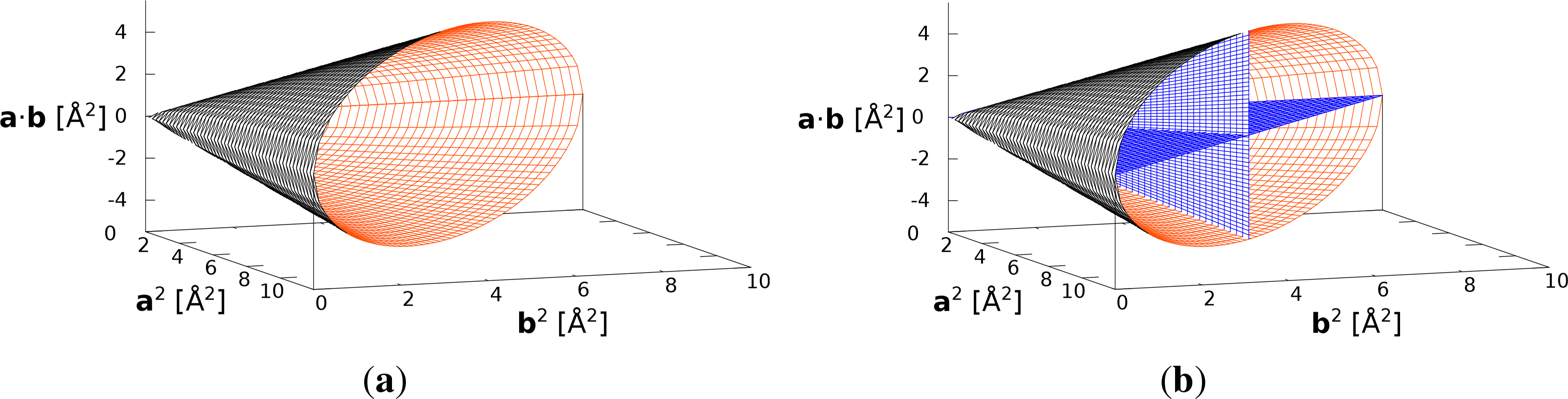
The lattice restriction imposed by the matrix P representing an isometry can be expressed by linear relationships between the scalar products ${\mathbf{a}}_i^2={\mathbf{a}}_j^2$, ${\mathbf{b}}_i^2={\mathbf{b}}_j^2$ and a_i · b_i = a_j · b_j. These relationships can be conveniently represented by the subspaces of the three-dimensional Euclidean space E³, where the three dimensions represent the elements of the metric tensor G_i, viz., ${\mathbf{a}}_i^2$, ${\mathbf{b}}_i^2$ and a_i · b_i, respectively. The metric tensor of a two-dimensional lattice is positive-definite, and the elements fulfill:

$${\mathbf{a}}_i^2>0$$

(5)

$${\mathbf{b}}_i^2>0$$

(6)

and

$${\left({\mathbf{a}}_i\cdot {\mathbf{b}}_i\right)}^2<{\mathbf{a}}_i^2{\mathbf{b}}_i^2$$

(7)

whereby the latter inequality can also be written as det(G_i) > 0. These ( ${\mathbf{a}}_i^2$, ${\mathbf{b}}_i^2$, a_i · b_i) triples describe an open, convex subset of E³. The boundary set is an elliptical cone with the apex located at the origin (Figure 2a). It is understood that if in the next sections, lattice restrictions are described as lines or planes in E³, actually, only the line or plane segment obtained by intersection with this subset represents two-dimensional lattices. Likewise, if a lattice parameter is said to be free, it may only be chosen such that the corresponding triple of scalar products is a member of this subset.

Since there is at least one free lattice parameter, the lattice restrictions can be expressed by a system of two linear equations according to:

$$\mathit{A}\left(\begin{array}{c}{\mathbf{a}}^2\\ {\mathbf{b}}^2\\ \mathbf{a}\cdot \mathbf{b}\end{array}\right)=\left(\begin{array}{ccc}{a}_{11}& a_{12}& a_{13}\\ a_{21}& a_{22}& a_{23}\end{array}\right)\left(\begin{array}{c}{\mathbf{a}}^2\\ {\mathbf{b}}^2\\ \mathbf{a}\cdot \mathbf{b}\end{array}\right)=\left(\begin{array}{c}0\\ 0\end{array}\right)$$

(8)

where A is a rational 2 × 3 matrix. A can be made unique by, for example, writing it in reduced row echelon form, i.e., applying the Gaussian elimination algorithm on the system of linear equations and making the leading non-zero elements of the matrix one. Three cases can be distinguished, based on the number of free parameters: if rank(A) = 0, all three lattice parameters are free; if rank(A) = 1, the solutions of the system of linear equations are located on a plane (two free parameters), which will be described by V, the coordinates of a vector normal to the plane. Finally, if rank(A) = 2, the solutions are located on a line passing through the origin (one free lattice parameter), which will be described by U, the coordinates of a vector parallel to this line. The three kinds of lattice restrictions are compiled in

Table 3. Possible matrix representations P of two-dimensional point group operations relating the lattices of L_i and L_j and the resulting restrictions of the lattice vectors, ordered by the number of free parameters.

Operation	det(P)	tr(P)	Free parameters	Lattice restriction
identity or two-fold rotation	1	±2	3	–
mirroring	−1	0	2	$\left({\mathbf{a}}_i^2,{\mathbf{b}}_i^2,{\mathbf{a}}_i\cdot {\mathbf{b}}_i\right)\mathit{V}=0,\hspace{0.17em}\mathit{V}=\left(\begin{array}{c}{V}_x\\ V_y\\ V_z\end{array}\right)=\left(\begin{array}{c}{p}_{12}\\ -p_{21}\\ -2p_{11}\end{array}\right)$
rotation by ψ ≠ = 0, π	1	| tr(P)| < 2	1	$\mathit{U}\times {\left({\mathbf{a}}_i^2,{\mathbf{b}}_i^2,{\mathbf{a}}_i\cdot {\mathbf{b}}_i\right)}^T=\mathit{o},\hspace{0.17em}\mathit{U}=\left(\begin{array}{c}{U}_x\\ U_y\\ U_z\end{array}\right)=\left(\begin{array}{c}2p_{21}\\ -2p_{12}\\ p_{22}-p_{11}\end{array}\right)$

and will be discussed in the following paragraphs based on the type of the lattice transformation represented by P.

2.4.1. Identity Operation or Two-Fold Rotation (Table 3, Line 1)

If P has the form P = ±I₂, i.e., it describes the identity operation or a two-fold rotation, the lattice is only restricted by Equations (5)–(7), since every two-dimensional lattice is symmetric by these two operations. Thus, the valid lattices are represented by a three-dimensional subset of E³ (Figure 2a). This is the lattice restriction of layer groups in the oblique lattice system.

2.4.2. Mirror Operation (Table 3, Line 2)

A matrix P representing a mirror operation fulfills:

$$\text{det}(\mathit{P})=-1$$

(9)

and

$$\text{tr}(\mathit{P})=p_{11}+p_{22}=0$$

(10)

The lattice restriction induced by P corresponds to a plane in E³, which is described by an equation:

$$\left({\mathbf{a}}_i^2,{\mathbf{b}}_i^2,{\mathbf{a}}_i\cdot {\mathbf{b}}_i\right)\mathit{V}=0$$

(11)

with V ≠ o. V can be derived from P (see Appendix 1.1) by:

$$\mathit{V}=\left(\begin{array}{c}{V}_x\\ V_y\\ V_z\end{array}\right)=\left(\begin{array}{c}{p}_{12}\\ -p_{21}\\ -2p_{11}\end{array}\right)$$

(12)

Since P is rational, so are the coefficients of V.

Two examples of this kind of restriction are depicted in Figure 2b: The horizontal plane represents the lattices fulfilling Equation (11) with V = (0, 0, 1)^T or a · b = 0 and the vertical plane V = (1, −1, 0)^T or a² = b². Lattices of the op and oc Bravais types of lattices (i.e., lattices of layers in both rectangular lattice systems) must fulfill these restrictions, respectively. Examples of non-crystallographic restrictions of this kind are given in Sections 2.12.1 and 2.12.2.

The set of solutions of Equation (11) contains ( ${\mathbf{a}}_i^2$, ${\mathbf{b}}_i^2$, a_i · b_i) triples of positive-definite G_i (i.e., the lattice restriction is valid), only if V fulfills:

$$V_x{V}_y<\frac{V_z^2}{4}$$

(13)

which is always the case for V of Equation (12), obtained from P fulfilling Equations (9) and (10). All V ≠ o representing parallel vectors (i.e., all λV, λ ≠ 0) describe the same lattice restriction. Notably, the equivalent lattice transformations represented by P and −P lead to the same lattice restriction (V and −V).

Since the matrix P representing a mirror operation must fulfill det(P) = −1 and tr(P) = 0, a lattice restriction of Equation (11) with given V is obtained from exactly two matrices P:

$$\mathit{P}=\frac{\pm 1}{l}\left(\begin{array}{cc}-\frac{V_z}{2}& V_x\\ -V_y& \frac{V_z}{2}\end{array}\right)$$

(14)

where

$$l=\sqrt{\frac{V_z^2}{4}-V_x{V}_y}>0$$

(15)

is a scale factor: l(V) = 1 for the form given in Equation (12) and l(λV) = |λ|l(V). V can be made unique by division by l and making V_x > 0. This form has the advantage that it can immediately be connected to the matrices ±P, which impose this restriction. Alternatively, the uniqueness of V can, for example, be achieved by making the elements integral, coprime and V_x > 0.

2.4.3. Rotation by ψ ≠ 0, π (Table 3, Line 3)

The matrix P representing a rotation by ψ ≠ 0, π has to fulfill:

$$\text{det}(\mathit{P})=1$$

(16)

and

$$\left|p_{11}+p_{22}\right|<2$$

(17)

since p₁₁ + p₂₂ = tr(P) = 2cos ψ. The lattice restriction imposed by such a matrix corresponds to a line in E³, which is described by the equation:

$$\mathit{U}\times {\left({\mathbf{a}}_i^2,{\mathbf{b}}_i^2,{\mathbf{a}}_i\cdot {\mathbf{b}}_i\right)}^T=\mathit{o}$$

(18)

with U ≠ o. Alternatively, the equation can be written as:

$$\left({\mathbf{a}}_i^2,{\mathbf{b}}_i^2,{\mathbf{a}}_i\cdot {\mathbf{b}}_i\right)=\lambda {\mathit{U}}^T$$

(19)

with λ ∈ ℝ. U can be deduced from P (see Appendix 1.1) by:

$$\mathit{U}=\left(\begin{array}{c}{U}_x\\ U_y\\ U_z\end{array}\right)=\left(\begin{array}{c}2p_{21}\\ -2p_{12}\\ -p_{11}+p_{22}\end{array}\right)$$

(20)

Since P is rational, so are the coefficients of U. The lattice restriction resulting from the identity or two-fold rotation (three free parameters) can be considered as a special case of Equations (18) and (20), since the corresponding matrices P = ±I₂ lead to U = o, and as a consequence, Equation (18) is always fulfilled. Nevertheless, it seems more clear to treat the unrestricted case as a distinct case, and here, only U ≠ o are considered.

An example of this kind of restriction is given by the intersection of the horizontal and the vertical plane in Figure 2b: this line represents the lattices fulfilling a² = b² and a · b = 0 or U = (1, 1, 0)^T, corresponding to the metrics of lattices of the tp Bravais types of lattices (lattices of layers in the square lattice system) in the reduced setting. An actual example of a non-crystallographic lattice restriction of this kind will be detailed in Section 2.12.3.

The set of solutions of Equation (18) contains ( ${\mathbf{a}}_i^2$, ${\mathbf{b}}_i^2$, a_i · b_i) triples of positive-definite G_i (i.e., the lattice restriction is valid) only if:

$$U_z^2<U_x{U}_y$$

(21)

which is always the case for U derived according to Equation (20) from matrices P fulfilling Equations (16) and (17). All U ≠ o representing parallel vectors (i.e., all λU, λ ≠ 0) describe the same lattice restriction. U can, for example, be made unique by making the elements integral and coprime and U_x positive. As opposed to the case of two free parameters, the lattice restrictions described byagiven U are derived from an infinity of matrices P. For example, the matrix representations:

$$\mathit{P}=\left(\begin{array}{cc}0& -1\\ 1& 0\end{array}\right)$$

(22)

and

$$\mathit{P}=\left(\begin{array}{cc}\frac{4}{5}& -\frac{3}{5}\\ \frac{3}{5}& \frac{4}{5}\end{array}\right)$$

(23)

of rotations by $\psi =\frac{\pi }{2}$ and $\psi ={\text{tan}}^{-1}\left(\frac{3}{4}\right)$, respectively, both lead to U = (1, 1, 0)^T (i.e., square lattices) (Figure 3).

2.5. Transformation of Lattice Restrictions

If the layers L_i and L_j are not equivalent, their lattices are related by:

$$\left({\mathbf{a}}_j,{\mathbf{b}}_j\right)=\left({\mathbf{a}}_i,{\mathbf{b}}_i\right)\left(\begin{array}{cc}{p}_{11}& p_{12}\\ p_{21}& p_{22}\end{array}\right)=\left({\mathbf{a}}_i,{\mathbf{b}}_i\right)\mathit{P}$$

(24)

with det(P) ≠ 0 (but not necessarily fulfilling det(P) = ±1). From VCβ″, it follows that P is rational. If the lattice of layer L_i is restricted as described in Section 2.4, additional restrictions are imposed on the lattice of layer L_j. To express the restriction in terms of the layer L_j, the need arises to apply lattice transformations to the representations of lattice restrictions introduced in Section 2.4. Moreover, in many cases, it is convenient to use different cell settings of a layer for structural descriptions. In these cases, P is usually integral, unless switching from a centered to a primitive setting. If V_i describes the restriction of the lattice of L_i according to Equation (11), then the lattice of L_j is likewise restricted according to Equation (11) with vector V_j related to V_i by:

$${\mathit{V}}_j=\left(\begin{array}{ccc}{p}_{22}^2& p_{12}^2& -p_{12}{p}_{22}\\ p_{21}^2& p_{11}^2& -p_{11}{p}_{21}\\ -2p_{21}{p}_{22}& -2p_{11}{p}_{12}& p_{11}{p}_{22}+p_{12}{p}_{21}\end{array}\right){\mathit{V}}_i$$

(25)

In analogy, the vector U_i of Equation (18) transforms according to:

$${\mathit{U}}_j=\left(\begin{array}{ccc}{p}_{11}^2& p_{12}^2& {2p}_{11}{p}_{21}\\ p_{21}^2& p_{22}^2& {2p}_{12}{p}_{22}\\ p_{11}{p}_{12}& p_{21}{p}_{22}& p_{11}{p}_{22}+p_{12}{p}_{21}\end{array}\right){\mathit{U}}_i$$

(26)

As expected, if V_i represents a valid lattice restriction (i.e., fulfills Equation (13)), then so does V_j, and likewise, if U_i fulfills Equation (21), then so does U_j, provided that det(P) ≠ 0, as is derived in Appendix 1.3. Moreover, the rationality of V_j and U_j is preserved for rational P.

2.6. Combination of Lattice Restrictions

The lattice of a layer may be restricted by symmetry operations (Section 2.3), σ-POs (Section 2.4) or the lattice restrictions of a different layer (Section 2.5). The combination (i.e., intersection) of these restrictions is used to determine the lattice restrictions of an OD family: a representative layer n-tuple of adjacent layers containing each kind of layer exactly once is considered. The lattices of all layers are expressed with respect to an arbitrarily chosen global lattice. The restrictions imposed by the layer symmetries and the σ-POs are transformed into the global lattice (Section 2.5) and combined. If the OD family is valid, the global lattice is described by one to three free parameters. This restriction is then transformed back into the lattice bases of the individual layers. As a consequence, in an OD family, every layer lattice has the same number of free parameters. For example, in an OD family containing a square layer, b/a and γ of all layers are fixed, even if they only belong to the oblique layer system. The combination of two lattice restrictions is compiled in

Table 4. Combination of lattice restrictions with V₁, V₂, U₁, U₂ ≠ o.

Restriction 1	Restriction 2	Condition	Resulting Restriction
(a2, b2, a · b)V1 = 0	(a2, b2, a · b)V2 = 0	V1 × V2 = o	(a2, b2, a · b)V1 = 0
(a2, b2, a · b)V1 = 0	(a2, b2, a · b)V2 = 0	$\mathit{U}=\left(\begin{array}{c}{U}_x\\ U_y\\ U_z\end{array}\right)={\mathit{V}}_1\times {\mathit{V}}_2{U}_z^2<U_x{U}_y$	U × (a2, b2, a · b)T = o
(a2, b2, a · b)V1 = 0	(a2, b2, a · b)V2 = 0	$\mathit{U}=\left(\begin{array}{c}{U}_x\\ U_y\\ U_z\end{array}\right)={\mathit{V}}_1\times {\mathit{V}}_2{U}_z^2\ge U_x{U}_y$	invalid
(a2, b2, a · b)V1 = 0	U2 × (a2, b2, a · b)T = o	${\mathit{V}}_1{\mathit{U}}_2^T=0$	U2 × (a2, b2, a · b)T = o
(a2, b2, a · b)V1 = 0	U2 × (a2, b2, a · b)T = o	${\mathit{V}}_1{\mathit{U}}_2^T\ne 0$	invalid
U1 × (a2, b2, a · b)T = o	U2 × (a2, b2, a · b)T = o	U1 × U2 = o	U1 × (a2, b2, a · b)T = o
U1 × (a2, b2, a · b)T = o	U2 × (a2, b2, a · b)T = o	U1 × U2 ≠ o	invalid

, and the different cases are detailed in the following sections, whereby the trivial cases (combination with no restrictions) are not listed.

2.6.1. Two Times Two Free Lattice Parameters (Table 4, Lines 1–3)

The lattice restrictions read as:

$$\left({\mathbf{a}}^2,{\mathbf{b}}^2,\mathbf{a}\cdot \mathbf{b}\right){\mathbf{V}}_k=0$$

(27)

with k = 1, 2. If the V_k represent parallel vectors (V₁ × V₂ = o), both restrictions are equivalent and, thus, identical to the resulting restriction. If V₁ × V₂ ≠ o, the number of free parameters is reduced to one. The possible lattices are described by Equation (18) with U = V₁ × V₂. An example is given in Figure 2b: the horizontal plane, described by V₁ = (0, 0, 1)^T, represents metrics of lattices in the op Bravais type of lattices and the vertical plane, described by V₂ = (1, −1, 0)^T, the metrics of lattices in the oc Bravais type of lattices. The intersection of these two planes is found by calculating U = V₁ × V₂ = (1, 1, 0)^T, which represents a line corresponding to the metrics of lattices in the tp Bravais type of lattices. Thus, if an OD structure is made up of orthorhombic primitive and orthorhombic c-centered layers and both layers possess the same (primitive) lattice, the lattices of both layers must be square.

Solutions with positive-definite G exist only for U fulfilling Equation (21). For example, a lattice cannot be restricted by a·b = 0 and $\mathbf{a}\cdot \mathbf{b}=\frac{1}{2}\mathbf{a}\cdot \mathbf{a}$ represented by V₁ = (0, 0, 1)^T and V₂ = (1, 0, −2)^T, respectively, since the resulting restriction represented by U = V₁ × V₂ = (0, −1, 0)^T corresponds to the lattice restriction a² = a · b = 0, which is not the case for any two-dimensional lattice. An example of the combination of lattice restrictions resulting in non-crystallographic lattice restrictions is given in Section 2.12.4.

2.6.2. Two and One Free Lattice Parameters (Table 4, Lines 4–5)

The lattice restrictions are given by:

$$\left({\mathbf{a}}^2,{\mathbf{b}}^2,\mathbf{a}\cdot \mathbf{b}\right){\mathbf{V}}_1=0$$

(28)

and:

$${\mathit{U}}_2\times {\left({\mathbf{a}}^2,{\mathbf{b}}^2,\mathbf{a}\cdot \mathbf{b}\right)}^T=\mathit{o}$$

(29)

If V₁ and U₂ represent perpendicular vectors ( ${\mathit{V}}_1{\mathit{U}}_2^T=0$), the second restriction is a strict subset of the first and accordingly equivalent to the resulting restriction. If ${\mathit{V}}_1{\mathit{U}}_2^T\ne 0$, only the trivial solution a² = b² = a · b = 0, which does not describe a two-dimensional lattice, is common to both restrictions.

2.6.3. Two Times One Free Lattice Parameter (Table 4, Lines 6–7)

The lattice restrictions read as:

$${\mathit{U}}_k\times {\left({\mathbf{a}}^2,{\mathbf{b}}^2,\mathbf{a}\cdot \mathbf{b}\right)}^T=\mathit{o}$$

(30)

with k = 1, 2. The restrictions are equivalent if the U_k are parallel (U₁ × U₂ = o) and, therefore, identical to the resulting restriction. If U₁ × U₂ ≠ o, only the trivial solution a² = b² = a · b = 0, which does not describe a two-dimensional lattice, is common to both restriction.

2.7. Expression of Lattice Restrictions in Terms of the Lattice Parameters

The lattice restrictions in terms of linear equations of the scalar products a², b² and a · b have been proven useful for the analysis of OD families. Nevertheless, an expression in terms of the lattice parameters a, b and γ may seem more natural. Moreover, one may be interested in the possible relative values of a and b. These expression are compiled in

Table 5. Layer lattice restriction expressed in the lattice parameters a, b and γ and example Bravais types of lattices in the standard primitive setting [21].

Lattice restriction	Subcase	a, b	γ	Example bravais Lattice
none	–	free	free	oblique
(a2, b2, a · b) V= 0, $\mathit{V}=\left(\begin{array}{c}{V}_x\\ V_y\\ V_z\end{array}\right)$	Vx = Vy = 0, Vz ≠ 0	free	$\frac{\pi }{2}$	rectangular primitive ( $\gamma =\frac{\pi }{2}$)
	Vx = 0, VyVz ≠ 0	$\frac{a}{b}>\left|\frac{V_y}{V_z}\right|$	${\text{cos}}^{-1}\left(-\frac{V_{y}b}{V_{z}a}\right)$
	Vy = 0, VxVz ≠ 0	$\frac{b}{a}>\left|\frac{V_x}{V_z}\right|$	${\text{cos}}^{-1}\left(-\frac{V_{x}a}{V_{z}b}\right)$
	VxVyVz ≠ 0	$\frac{b}{a}\in \left(\frac{\left|V_z\right|-2l}{2\left|V_y\right|},\frac{\left|V_z\right|+2l}{2\left|V_y\right|}\right)$	${\text{cos}}^{-1}\left(-\frac{V_{x}a}{V_{z}b}-\frac{V_{y}b}{V_{z}a}\right)$
	Vz = 0	$b=\sqrt{\frac{V_y}{V_x}}a$	free	rectangular c-centered (a = b)
U × (a2, b2, a · b))T = o, $\mathit{U}=\left(\begin{array}{c}{U}_x\\ U_y\\ U_z\end{array}\right)$	–	$b=\sqrt{\frac{U_y}{U_x}}a$	${\text{cos}}^{-1}\left(\frac{U_z}{\sqrt{U_x{U}_y}}\right)$	hexagonal (a = b, $\gamma =\frac{2\pi }{3}$), square (a = b, $\gamma =\frac{\pi }{2}$)

Note: l is the scale factor defined in Equation (15).

and will be described in detail in the next paragraphs.

2.7.1. Two Free Parameters (Table 5, Lines 2–6)

To express Equation (11) in terms of the lattice parameters, two cases have to be distinguished: V_z ≠ 0 (Table 5, Lines 2–5) and V_z = 0 (Table 5, Line 6). If V_z ≠ 0, Equation (11) can be written as:

$$\mathbf{a}\cdot \mathbf{b}=-\frac{V_x{\mathbf{a}}^2+V_y{\mathbf{b}}^2}{V_z}$$

(31)

which translates into:

$$\gamma ={\text{cos}}^{-1}\left(-\frac{V_{x}a}{V_{z}b}-\frac{V_{y}b}{V_{z}a}\right)$$

(32)

Concerning the restrictions of the relation between a and b, there are four subcases: If V_x = V_y = 0, then $\gamma =\frac{\pi }{2}$ and a > 0 and b > 0 are free. If V_x = 0, V_y ≠ 0, then $\frac{a}{b}>\left|\frac{V_y}{V_z}\right|$. If V_x ≠ 0, V_y = 0, then $\frac{b}{a}>\left|\frac{V_x}{V_z}\right|$. If V_xV_y ≠ 0, then:

$$\frac{b}{a}\in \left(\frac{\left|V_z\right|-2l}{2\left|V_y\right|},\frac{\left|V_z\right|+2l}{2\left|V_y\right|}\right)$$

(33)

where l is the scale factor defined in Equation (15).

If V_z = 0, Equation (11) can be written as:

$$b=\sqrt{-\frac{V_y}{V_x}a}$$

(34)

and γ is free. This case corresponds to the lattice transformation where the mirror line is the bisector of a_i ∧ b_i. An example is the standard primitive setting of centered rectangular lattices where a = b [21].

2.7.2. One Free Parameter (Table 5, Line 7)

Equation (18) can be written in terms of a, b and γ as:

$$b=\sqrt{\frac{U_y}{U_x}a}$$

(35)

and

$$\gamma ={\text{cos}}^{-1}\left(\frac{U_z}{\sqrt{U_x{U}_y}}a\right)$$

(36)

2.8. Determinateness of Transformation Matrices

To interpret the layer group and OD groupoid family symbols (see Section 2.10), the printed symbols for symmetry elements [22] must be converted into transformation matrices. Since the linear part M of any PO can only take the form of Equation (3), the task is reduced to determining the matrix P, representing the two-dimensional lattice transformation, and extending it by m₃₃ = ±1, depending on the type of operation. If the lattice restriction of the OD family is defined sufficiently, P is unambiguous and independent of the lattice parameters a, b and γ. The matrices representing rotations by ψ = 0, π are always unambiguously defined. In any basis, the corresponding matrix reads as:

$$\mathit{P}=\pm {\mathit{I}}_2$$

(37)

2.8.1. Two Free Parameters

If the geometry of a lattice is restricted according to Equation (11), it can be unambiguously associated with two mirror operations represented by the matrix ±P′ according to Equation (14). The matrix representing a mirror operation is only unambiguously defined if the latter is one of these two operations, as derived in Appendix 1.4. Thus, only mirror operations at lines that are left invariant by the operations represented by ±P′ are unambiguously defined. The matrix representation P of a mirror operation at a line parallel to ua + vb is:

$$\mathit{P}=\{\begin{array}{ll}\mathit{P}\prime \hfill & \text{if}\hspace{0.17em}\mathit{P}\prime \left(\begin{array}{l}u\\ v\end{array}\right)=\left(\begin{array}{l}u\\ v\end{array}\right)\hfill \\ -\mathit{P}\prime \hfill & \text{if}-\mathit{P}\prime \left(\begin{array}{l}u\\ v\end{array}\right)=\left(\begin{array}{l}u\\ v\end{array}\right)\hfill \end{array}$$

(38)

or dependent on the actual lattice metrics otherwise. The matrix representing a rotation by ψ ≠ 0, π is never unambiguously defined if there are two free lattice parameters.

2.8.2. One Free Parameter

The matrices representing mirror operations at a line parallel to ua + vb and normal to ua + vb and rotations by ψ are given in

Table 6. Matrices P representing two-dimensional lattice transformations if the lattice restriction reads as U × (a², b², a · b)^T = o (one free parameter).

Operation	P
Mirror at a line parallel to ua + vb	$\frac{1}{o}\left(\begin{array}{cc}m-n\frac{U_z}{U_x}& n\left(\frac{U_y}{U_x}-2\frac{U_z^2}{U_x^2}\right)+2m\frac{U_z}{U_x}\\ n& -m+n\frac{U_z}{U_x}\end{array}\right)†$
Mirror at a line normal to ua + vb	$\frac{1}{o}\left(\begin{array}{cc}-m+n\frac{U_z}{U_x}& -n\left(\frac{U_y}{U_x}-2\frac{U_z^2}{U_x^2}\right)-2m\frac{U_z}{U_x}\\ -n& m-n\frac{U_z}{U_x}\end{array}\right)†$
Rotation by ψ	$\left(\begin{array}{cc}\text{cos}\psi -\frac{U_z\text{sin}\psi }{\sqrt{U_x{U}_y-U_z^2}}& -\frac{U_y\text{sin}\psi }{\sqrt{U_x{U}_y-U_z^2}}\\ \frac{U_x\text{sin}\psi }{\sqrt{U_x{U}_y-U_z^2}}& \text{cos}\psi +\frac{U_z\text{sin}\psi }{\sqrt{U_x{U}_y-U_z^2}}\end{array}\right)$

Note: $m=u^2+v^2\frac{2U_z^2-U_x{U}_y}{U_x^2}+2uv\frac{U_z}{U_x},n=2\left(uv+u^2\frac{U_z}{U_x}\right),o=u^2+v^2\frac{U_y}{U_x}+2uv\frac{U_z}{U_x}$.

and derived in Appendix 1.4.

2.9. Representation Using Centered Lattices

For convenience, crystallographers commonly use the concept of centered lattices. For example, a rectangular centered lattice (a′, b′) is decomposed into the 0 and $\frac{1}{2}(\mathbf{a}+\mathbf{b})$ cosets of a primitive rectangular sublattice (a, b). Whereas using primitive lattices over centered lattices generally simplifies computational problems and mathematical reasoning, since there is no need to keep track of centering vectors, centered lattices may be more descriptive. Thus, in the following paragraphs, possible centered settings will be described, excluding the three free parameter case.

2.9.1. Two Free Parameters

If the lattice of a layer L_i is restricted according to Equation (11), the restriction can be associated with two mirror operations at perpendicular lines, represented by the matrices ±P of Equation (14). Thus, a description that suggests itself is in terms of rectangular centered lattices: since P is rational, both perpendicular mirror lines are parallel to an infinity of non-zero lattice vectors. The shortest of these two sets of vectors, a′_i and b′_i, span a rectangular lattice 𝔏′, which is invariant under the application of the mirror operations represented by ±P. As expected, also in this setting, there are two free lattice parameters, viz., a = |a′| and b′ = |b′|, whereas $\gamma \prime =\mathbf{a}\prime ^\mathbf{b}\prime =\frac{\pi }{2}$ is fixed.

The coset decomposition of 𝔏′ in 𝔏_i furnishes the centering vectors of L_i. If the coset decompositions are {𝔏′} or { $𝔏\prime ,\frac{1}{2}\left({\mathbf{a}\prime }_i+{\mathbf{b}\prime }_i\right)𝔏\prime$}, then 𝔏_i is a rectangular primitive or a rectangular c-centered lattice, respectively. In these two cases, the lattice 𝔏_j generated from 𝔏_i by the operation represented by P is identical to 𝔏_i. In all other cases, 𝔏_i ≠ 𝔏_j.

The intersection 𝔏_i ∩ 𝔏_j is invariant under the mirror operation described by P, and therefore, it is always either a rectangular primitive or a rectangular c-centered lattice: if u ∈ 𝔏_i ∩ 𝔏_j, then u ∈ 𝔏_j, and thus, it was generated from a vector u′ ∈ 𝔏_i. Since P² = I₂, the mirror image of u ∈ 𝔏_i is u′ ∈ 𝔏_j. Thus, u′ ∈ 𝔏_i ∩ 𝔏_j.

2.9.2. One Free Parameter

As has been shown in Section 2.4.3, a lattice restriction with one free parameter cannot be related to a unique transformation matrix P, and thus, the choice of a suitable basis is not as obvious as in the case of two free parameters. In OD families fulfilling VCβ, the sublattice common to all polytypes is an obvious choice. Otherwise, if square or hexagonal sublattices can be found, these would probably represent a good bases for centered lattices (the centering vectors are again determined by coset-decomposition).

For any lattice restricted according to Equation (18), a rectangular sublattice can be found: Since U_x, U_z ∈ ℚ, from Equation (18), it follows that the ratio of a_i · b_i to ${\mathbf{a}}_i^2$ is rational:

$${\mathbf{a}}_i\cdot {\mathbf{b}}_i=\frac{q{\mathbf{a}}_i^2}{r}$$

(39)

with q ∈ ℤ, r ∈ ℤ \ {0}. Thus, (a_i, qa_i − rb_i) spans a rectangular sublattice (which is not necessarily the largest rectangular sublattice of 𝔏_i). For example, a hexagonal lattice can always be represented by rectangular c-centered lattices with $b=\sqrt{3}a$ (or $a=\sqrt{3}b$) (Figure 4). Nevertheless, as opposed to the case of two free parameters, this is not necessarily a convenient setting. Indeed, hexagonal lattices are usually described in the primitive setting, since it is more descriptive.

2.10. Extension of the Notation for OD Groupoid Families

Symbols describing OD groupoid families based on the Hermann–Mauguin notation were developed by Dornberger–Schiff and Grell–Niemann [8,13] for OD families fulfilling VCβ′. A shortening and an update of the notation was proposed by Fichtner [4,23]. Until a more general notation is developed, a few ad hoc adaptations are proposed below to enable the description of OD groupoid families fulfilling only VCβ or VCβ′.

2.10.1. Notation for Layers with All of the Same Lattice (VCβ′)

As has been stated in Section 2.3, if the layers of an OD family all feature the same lattice, the latter must be invariant under application of any σ-or λ-PO. Therefore, the OD family can be associated with one of the five two-dimensional Bravais types of lattices [16], and all σ- and λ-POs only appear in the directions of the crystallographic point groups (with the exception of cubic point groups, which are not possible for layers). The OD groupoid symbol contains the Hermann–Mauguin symbol of the layer group type of every kind of layer. The direction lacking translational symmetry is indicated by parentheses. The σ-POs are listed in curly braces below or besides the layer group symbols. The direction is implicitly derived from the place in the symbol. For tetragonal, trigonal and hexagonal OD families, five- and seven-placed symbols are used, since the σ-POs are not necessarily equivalent in all directions of {110} or {120}. If the translational components of the σ-POs are not indicated by intrinsic translations of screws or glides, they are specified additionally in brackets. The bracket-notation is likewise used for adjacent layers of different kind. Examples of OD groupoid family symbols composed of layers of one and two kinds are:

$$\begin{array}{ccccccc}p& 2& 2& (4)& 2& 2& \\ \{& n_{r-s,2}& n_{2,r+s}& \left(\begin{array}{c}{\overline{4}}^{+}\\ {\overline{4}}^{-}\\ n_{r+s,r-s}\end{array}\right)& n_{2,s}& n_{2,-r}& \}\end{array}$$

(40)

and

$$\begin{array}{ccc}pmm(m)& & pmm(m)\\ & [r,s]& \end{array}$$

(41)

Equation (40) describes an OD family made up of layers of one kind with tetragonal p(4)22 symmetry. The operations of the layer group and the σ-POs are given in the [100], [010], [001], [110] and [11̄0] directions. Thus, given a layer L_i, one possible orientation of the adjacent layer L_j is related to L_i by four-fold rotoinversions or by glides with planes parallel to either of the five given directions. Equation (41) describes an OD family made up of layers of two kinds, both with orthorhombic pmm(m) symmetry and the same lattice. The origins of the layer L_i and of one possible orientation of the adjacent layer L_j are connected by the vector ra_i + sb_i + c₀, where c₀ is a vector normal to the layer planes.

2.10.2. Adapted Notation

In OD families with partially overlapping layer lattices, σ-POs can appear in arbitrary (rational) directions. If they appear in non-crystallographic directions, the notation for OD families described above is not adequate. Therefore, it is proposed to list all symmetry elements in the same direction in columns with the direction given in the column head. The σ-POs are listed besides, not below, the layer group symbols, since the positions in the layer group symbol and the σ-PO list do not stand for the same direction. As an example consider the symbol of an OD groupoid family of non-polar layers:

$$p(\overline{4})11\left\{\begin{array}{cccc}[120]& [2\overline{1}0]& [1\overline{3}0]& [310]\\ 2_s& 2_r& n_{2,\frac{r}{2}+\frac{s}{2}}& n_{2,\frac{r}{2}-\frac{s}{2}}\end{array}\right\}$$

(42)

Note that since the positions of the layer group symbol are not used for the σ-POs, the tetragonal layer group is indicated using the usual three-placed symbol. In this case, the σ-POs are listed only up to the lattice of the layer and not relative to the common sublattice of both adjacent layers to save space.

To indicate the relationship of the lattices of layers of different kinds, the base (a′, b′) of the layer is expressed in terms of the base (a, b) of a (arbitrarily chosen) global lattice either in the subscript of the Bravais symbol or in curly braces after the Bravais symbol. Thus, the layer group symbol may read as:

$$p\{\mathbf{a}\prime =\mathbf{a}+\mathbf{b},\mathbf{b}\prime =\mathbf{a}-\mathbf{b}\}\mathit{nm}(a)$$

(43)

or

$$p_{\mathbf{a}\prime =\mathbf{a}+\mathbf{b},\mathbf{b}\prime =\mathbf{a}-\mathbf{b}}\mathit{nm}(a)$$

(44)

Finally, as has been stated in Section 2.8, the direction and rotation angle of a σ-PO does, in some cases, not fully describe the operation. It may, therefore, be necessary to indicate additional restrictions of the global lattice. If the global lattice is restricted according to Equation (11) (two free parameters), it is chosen to be rectangular, as described in Section 2.9. The rectangular lattice restriction is indicated by writing “op”—the symbol for the rectangular primitive Bravais type of lattices [21]—in front of the OD groupoid family symbol. If the global lattice is restricted according to Equation (18) (one free parameter), the restriction of the global lattice is written in front of the OD-family symbol in angle brackets. Depending on the case, this may be more favorably done in terms of vectors or lattice parameters: e.g., “〈a · b = $-\frac{{\mathbf{a}}^2}{2}$, b² = a²〉” or “〈a = b, γ = 120^°〉”. The primitive settings of the square (〈a · b = 0, b² = a²〉) and hexagonal (〈a · b = $-\frac{{\mathbf{a}}^2}{2}$, b² = a²〉) lattices may be abbreviated by the symbols tp and hp of the corresponding Bravais types of lattices [21]. An example where the specification of the lattice restriction and the indication of the location of the layer relative to the global lattice is necessary is given in Section 2.12.2.

2.11. Basis-Independent Classification of Lattice Restrictions

The lattice restrictions presented in the previous sections were expressed in terms of scalar products of the basis vectors and, thus, are dependent on the choice of the (primitive) basis. To compare two lattice restrictions for equivalence (i.e., the existence of primitive settings in which both restrictions are identical) in the case of two free parameters, the lattices are expressed as centered rectangular lattices, as described in Section 2.9.1, and the centering vectors are compared (taking into account the permutations of the basis vectors). In the case of only one free parameter, a canonical representation of both lattice restrictions obtained by lattice reduction is compared.

2.12. Examples

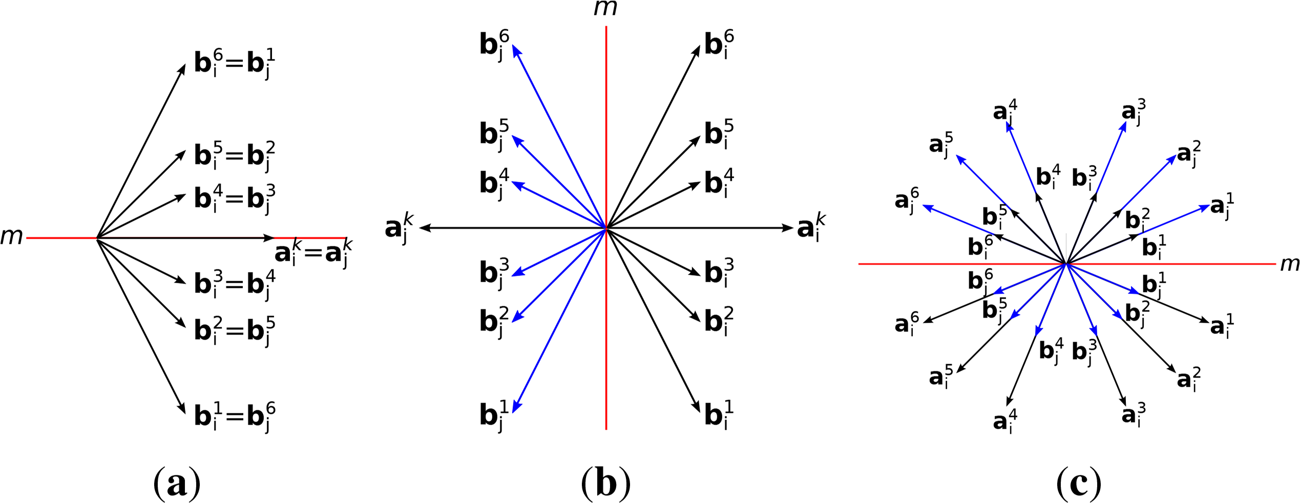
2.12.1. Example 1: Lattice Restrictions Induced by Mirror Operations

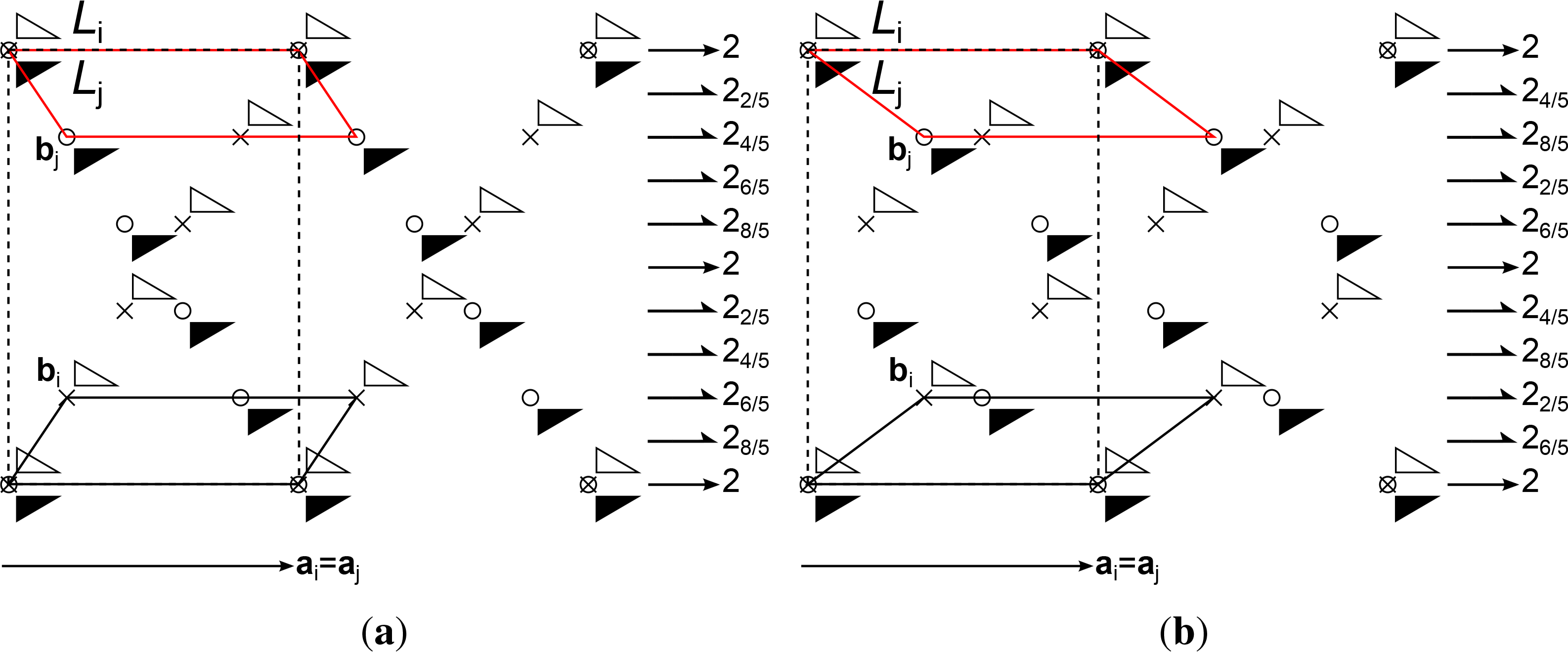
In Figure 5, the lattice basis vectors of three times six different pairs of layers ( $L_i^k$, $L_j^k$), k = 1,..., 6, where the lattices of $L_i^k$ and $L_j^k$ are related by mirror operations, are represented. The mirror line is parallel to a_i (Figure 5a), normal to a_i (Figure 5b) or the bisector of a_i ∧ b_i (Figure 5c). In all three cases, there are two free parameters, and the lattice restriction can be written as in Equation (11) with V = (−1, 0, 2)^T (Figure 5a,b) and V = (1, −4, 0)^T (Figure 5c). Whereas the σ-POs in Figure 5a,b are different, the lattice transformations and, as a consequence, the lattice restrictions in both cases are equivalent, since mirroring at a line and at the perpendicular line are equivalent lattice transformations. In the examples of Figure 5a,b, if a_i is fixed, then the end point of b_i can be moved along a line normal to a_i. In Figure 5c, |b_i|/|a_i| is fixed and the angle γ_i = a_i ∧ b_i is free. In terms of the lattice parameters a, b, γ, the lattice restrictions read as $b>\frac{a}{2}$, $\gamma ={\text{cos}}^{-1}\left(\frac{a}{2b}\right)$ (Figure 5a,b) and a = 2b (Figure 5c).

2.12.2. Example 2: POs of the Same Kind, Different OD Families

In Figure 6, two pairs of equivalent layers ( $L_i^k$, $L_j^k$), k = 1, 2 with symmetry p11(1) are schematized. In both cases, $L_i^k$ and $L_j^k$ are related by screws and rotations with axes parallel to [100] (expressed in the coordinate system of either layer or the common lattice of both layers) and intrinsic translation vectors $\frac{n{\mathbf{a}}_i}{5}$ with n = 0, 1, 2, 3, 4. Nevertheless, both figures represent different OD families. In Figure 6a, the linear part of the σ-POs expressed in the coordinate system of layer L_i is:

$$\mathit{M}=\left(\begin{array}{ccc}1& \frac{2}{5}& 0\\ 0& \overline{1}& 0\\ 0& 0& \overline{1}\end{array}\right)$$

(45)

whereas it is:

$$\mathit{M}=\left(\begin{array}{ccc}1& \frac{4}{5}& 0\\ 0& \overline{1}& 0\\ 0& 0& \overline{1}\end{array}\right)$$

(46)

in Figure 6b. Both cases can be distinguished by the restriction of the lattices. Since the lattices are related by a mirror operation, there are two free parameters and the lattices are restricted according to Equation (11) with V = (−1, 0, 5)^T (Figure 6a) and V = (−2, 0, 5)^T (Figure 6b). These restrictions expand to ${\mathbf{a}}_i\cdot {\mathbf{b}}_i=\frac{{\mathbf{a}}_i^2}{5}$, and ${\mathbf{a}}_i\cdot {\mathbf{b}}_i=\frac{2{\mathbf{a}}_i^2}{5}$, respectively. To describe the layer stacking according to the ad hoc notation of Section 2.10, the layers are expressed relative to global rectangular lattices (a_i, 5b_i − a_i) and (a_i, 5b_i − 2a_i), whose unit cells are indicated by dashed lines in Figure 6. Since the given layers are polar, a second layer contact is needed to fully describe an OD family. If the other sides of the layers contact via a glide with the plane parallel to the layer planes, the proposed OD groupoid family symbols read as:

$$\begin{array}{ccccccc}O& p_{\mathbf{b}\prime =\frac{\mathbf{a}}{5}+\frac{\mathbf{b}}{5}}& \begin{array}{ccc}1& 1& (1)\end{array}& & O& p_{\mathbf{b}\prime =\frac{2\mathbf{a}}{5}+\frac{\mathbf{b}}{5}}& \begin{array}{ccc}1& 1& (1)\end{array}\\ & & \left\{\begin{array}{ccc}{2}_{r\prime }& & \\ 2_{\frac{2}{5}+r\prime }& & \\ 2_{\frac{4}{5}+r\prime }& -& (-)\\ 2_{\frac{6}{5}+r\prime }& & \\ 2_{\frac{8}{5}+r\prime }& & \end{array}\right\}& \text{and}& & & \left\{\begin{array}{ccc}{2}_{r\prime }& & \\ 2_{\frac{2}{5}+r\prime }& & \\ 2_{\frac{4}{5}+r\prime }& -& (-)\\ 2_{\frac{6}{5}+r\prime }& & \\ 2_{\frac{8}{5}+r\prime }& & \end{array}\right\}\\ & & \begin{array}{ccccc}\{& -& -& \left(n_{r,s}\right)& \}\end{array}& & & & \begin{array}{ccccc}\{& -& -& \left(n_{r,s}\right)& \}\end{array}\end{array}$$

(47)

with r′ = 0 in the example of Figure 6. Since the axes of the screws are parallel to the [100] direction, the directions of the POs can be given implicitly by the position in the symbol. If the rectangular sublattice is chosen as the setting of the layers, they possess non-Bravais centering with four centering vectors $\frac{n}{5}(\mathbf{a}+\mathbf{b})$ and $\frac{n}{5}(2\mathbf{a}+\mathbf{b})$ (n = 1, 2, 3, 4), respectively.

2.12.3. Example 3: KOH·2H₂O

Partially overlapping layer lattices related by rotation are observed in KOH·2H₂O. The structure belongs to an OD family of non-polar layers of one kind. The layers possess orthorhombic symmetry pbm(a). Adjacent layers are related by four-fold screws with the axis parallel to the stacking direction [001] (Figure 7). Therefore, the lattices are restricted according to Equation (18), and there is only one free lattice parameter. In this case, U = (1, 4, 0)^T, or in terms of the lattice parameters: b = 2a, $\gamma =\frac{\pi }{2}$. The linear part of the $4_{4̄}$ operation relating L_i and L_j reads as:

$$\mathit{M}=\left(\begin{array}{ccc}0& 2& 0\\ \frac{\overline{1}}{2}& 0& 0\\ 0& 0& 1\end{array}\right)$$

(48)

The square lattice (a, b) = (2a_i, b_i) is common to all layers (VCβ is fulfilled), and therefore, the structure is best described in terms of this lattice. The OD groupoid family symbol then reads as:

$$tp{p}_{\mathbf{a}\prime =2\mathbf{a}}bm(a)\left\{\begin{array}{ccc}[2\overline{1}0]& [210]& [001]\\ 2_r& 2_{\frac{3}{4}+s}& 4_4^{+}\\ 2_{\frac{1}{2}+r}& 2_{\frac{5}{4}+s}& 4_4^{-}\\ n_{2,\frac{1}{2}-s}& n_{2,\frac{7}{4}+r}& {\overline{4}}^{+}\\ n_{2,1-s}& n_{2,\frac{1}{4}+r}& {\overline{4}}^{-}\end{array}\right\}$$

(49)

Note that the directions of the σ-POs are given with respect to the layer lattices, not the common square sublattice. The intrinsic translations are given with respect to the primitive lattice vector in the given direction. For example, the intrinsic translations along [210] are given relative to 2a_i + b_i = a + b. In the actual structure, $(r,s)=\left(\frac{1}{2},\frac{1}{4}\right)$; thus, one possible orientation of the layer L_j is generated from L_i by a screw with intrinsic translation $\frac{1}{2}(\mathbf{a}+\mathbf{b})=\left({\mathbf{a}}_i+\frac{{\mathbf{b}}_i}{2}\right)$.

2.12.4. Example 4: Layers of Different Kinds

In Figure 8, three different OD families composed of an alternating stacking of non-polar layers of two kinds are depicted. All layers possess p2m(m) symmetry. The basis (a_j, b_j) of one possible orientation of layer $L_j^k$, k = 1, 2, 3 is related to the basis (a_i, b_i) of layer $L_i^k$ by (a_j, b_j) = (a_i − b_i, a_i + b_i) (Figure 8a), (a_j, b_j) = (a_i−2b_i, 2a_i+b_i) (Figure 8b) and (a_j, b_j) = (a_i−b_i, 2a_i+b_i) (Figure 8c). Due to the orthorhombic layer group p2m(m), each layer lattice must be rectangular (a_i · b_i = a_j · b_j = 0). Moreover, according to the rules given in Section 2.6, the lattices must be square in Figure 8a,b (a_i = b_i, a_j = b_j, γ_i = γ_j = ${\gamma }_i={\gamma }_j=\frac{\pi }{2}$) or fulfill $b_i=\sqrt{2}{a}_i$, $b_j=\sqrt{2}{a}_j$, ${\gamma }_i={\gamma }_j=\frac{\pi }{2}$ in Figure 8c. Thus, the lattices are restricted according to Equation (18) with U = (1, 1, 0)^T (Figure 8a,b) and U = (1, 2, 0)^T (Figure 8c). Although, in all three cases, the layers $L_i^k$ and $L_j^k$ are restricted by the same lattice restrictions, the individual layers of each pair feature different lattice metrics. The lattice parameters are linked by $a_j=\sqrt{2}{a}_i$ (Figure 8a), $a_j=\sqrt{5}{a}_i$ (Figure 8b) and $a_j=\sqrt{3}{a}_i$ (Figure 8c). In the OD family depicted in Figure 8a, the lattice 𝔏_j is a common sublattice of all layers. Thus, the OD family fulfills VCβ. The point group of the family (the group generated by the linear parts of all POs [10]) is 422. In the examples in Figure 8b,c, on the other hand, polytypes with no translational symmetry exist; thus, only VCβ″ is fulfilled. The non-crystallographic point groups of both cases are written as ∞2 (The equivalence of such point groups is not obvious. Consider, for example, the point groups of rotations by $\psi =q\pi /\sqrt{2}$ and by $\psi =q\pi /\sqrt{3}$, q ∈ ℚ, which would both be written as ∞, but possess only one common element). The OD family symbols could be written according to the modifications of Section 2.10 as:

$$\begin{array}{cccc}\mathit{tp}& p2m(m)& & p_{\mathbf{a}\prime =\mathbf{a}+\mathbf{b},\mathbf{b}\prime =\mathbf{a}-\mathbf{b}}2/m1(1)\\ & & [r,s]& \end{array}\hspace{0.17em}\hspace{0.17em}\hspace{0.17em}\hspace{0.17em}\hspace{0.17em}(\text{Figure}\hspace{0.17em}8\text{a})$$

(50)

$$\begin{array}{cccc}\mathit{tp}& p2m(m)& & p_{\mathbf{a}\prime =2\mathbf{a}+\mathbf{b},\mathbf{b}\prime =\mathbf{a}-2\mathbf{b}}2/m1(1)\\ & & [r,s]& \end{array}\hspace{0.17em}\hspace{0.17em}\hspace{0.17em}\hspace{0.17em}\hspace{0.17em}(\text{Figure}\hspace{0.17em}8\text{b})$$

(51)

$$\begin{array}{cccc}\langle \mathbf{a}\cdot \mathbf{b}=0,{\mathbf{b}}^2=2{\mathbf{a}}^2\rangle & p2m(m)& & p_{\mathbf{a}\prime =2\mathbf{a}+\mathbf{b},\mathbf{b}\prime =\mathbf{a}-2\mathbf{b}}2/m1(1)\\ & & [r,s]& \end{array}\hspace{0.17em}\hspace{0.17em}\hspace{0.17em}(\text{Figure}\hspace{0.17em}8\text{c})$$

(52)

The indication of the lattice restriction is redundant, since it can be deduced from the symmetry groups and the relations of the layers. Nevertheless, it is spelled out for clarity.

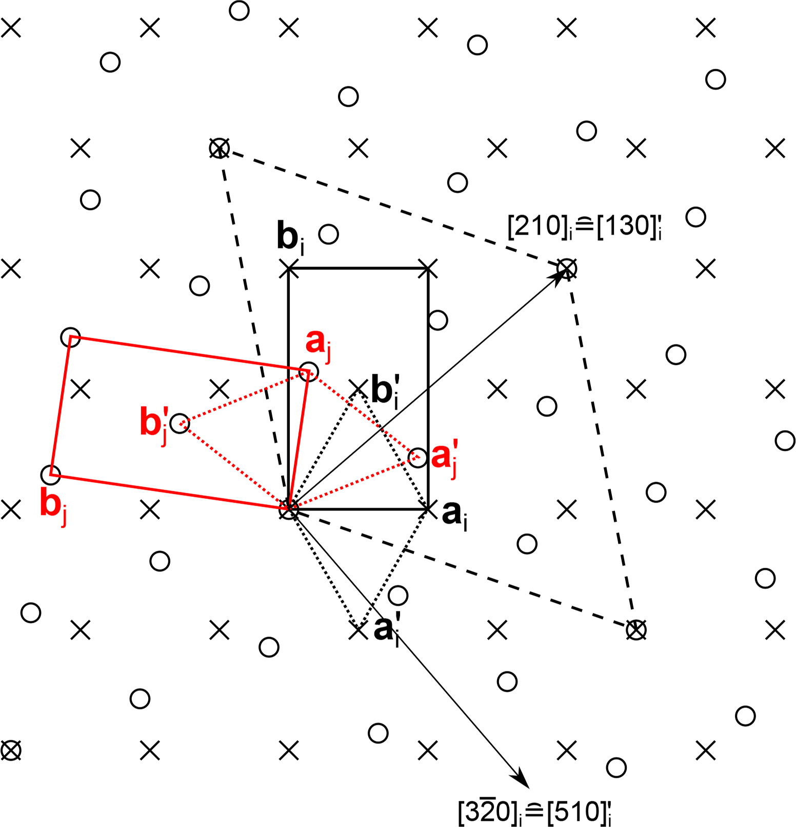
2.12.5. Example 5: Centered Layers

In Figure 9, the lattices of two equivalent layers L_i and L_j with c22(2) symmetry are represented by crosses and circles, respectively. The bases of the centered setting of the layers are (a_i, b_i) and (a_j, b_j) and the lattice parameters a, b and γ. The transformation matrix with respect to (a_i, b_i) reads as:

$$\mathit{P}=\left(\begin{array}{cc}\frac{1}{7}& \frac{\overline{12}}{7}\\ \frac{4}{7}& \frac{1}{7}\end{array}\right)$$

(53)

Substitution into Equation (20) and simplification by common factors leads to U = (1, 3, 0)^T or $b=\sqrt{3}a$, $\gamma =\frac{\pi }{2}$. The transformation matrix with respect to the primitive basis $\left({\mathbf{a}\prime }_i,{\mathbf{b}\prime }_i\right)=\frac{1}{2}(\mathbf{a}-\mathbf{b},\mathbf{a}+\mathbf{b})$ of the L_i layer reads as:

$$\mathit{P}\prime =\left(\begin{array}{cc}\frac{3}{7}& \frac{\overline{8}}{7}\\ \frac{8}{7}& \frac{\overline{5}}{7}\end{array}\right)$$

(54)

Substitution into Equation (20) and simplification by common factors leads to U = (1, 1, −2)^T or in terms of the lattice parameters: b′ = a′, $\gamma \prime =\frac{2\pi }{3}$. Thus, the primitive settings of the L_i and L_j layers possess hexagonal metrics, and in this example, the expression of the symmetry operations may be more convenient in the primitive setting. Expression of centered layer groups in the primitive setting is in principle realized in the seven-placed OD groupoid symbols of hexagonal and trigonal OD families. The largest common lattice 𝔏_i ∩ 𝔏_j of the L_i and L_j layers is spanned by (a″, b″) = (3a′_i +2b′_i, −2a′_i + b′_i) and likewise possesses hexagonal metrics. This is indicated in Figure 9 by dashed lines. The matrices P and P represent a rotation by $\psi ={\text{cos}}^{-1}\left(\frac{1}{7}\right)$. Using the generalization of the printed symbols for screws [8], the adapted OD groupoid family symbol could be written as:

$$<b=\sqrt{3}a,\gamma =\frac{\pi }{2}>c22(2)\left\{\begin{array}{ccc}[001]& [210]& [3\overline{2}0]\\ 2\pi /{\text{cos}}^{-1}{\left(\frac{1}{7}\right)}_{2\pi /{\text{cos}}^{-1}\left(\frac{1}{7}\right)}^{+}& 2_r& 2_s\\ 2\pi /{\text{cos}}^{-1}{\left(-\frac{1}{7}\right)}_{2\pi /{\text{cos}}^{-1}\left(-\frac{1}{7}\right)}^{-}& 2_{r+\frac{5}{7}}& 2_{s+\frac{12}{7}}\end{array}\right\}$$

(55)

or, perhaps more concisely, using the seven-placed notation as:

$$hpp211(2)211\left\{\begin{array}{ccc}[001]& [130]& [510]\\ 2\pi /{\text{cos}}^{-1}{\left(\frac{1}{7}\right)}_{2\pi /{\text{cos}}^{-1}\left(\frac{1}{7}\right)}^{+}& 2_r& 2_s\\ 2\pi /{\text{cos}}^{-1}{\left(-\frac{1}{7}\right)}_{2\pi /{\text{cos}}^{-1}\left(-\frac{1}{7}\right)}^{-}& & \end{array}\right\}$$

(56)

Clearly, the usual notation for screws and rotations is cumbersome for non-crystallographic rotation angles, and further adaptations are needed. The non-crystallographic point group of the OD family is ∞2.

3. Conclusions

It has been shown that operations relating equivalent layers in OD families, as well as the existence of non-equivalent layers lead to lattice restrictions that can be expressed as linear relations of the scalar products of the lattice basis vectors with rational coefficients. These relations are a concise and convenient computational device for the analysis of OD families. Nevertheless, these considerations only scratch the surface of a theory of OD structures composed of layers with different translational groups, and significantly more work is needed. For example, a classification of OD families based on these restrictions in analogy to the assignment of symmetry groups to Bravais types of lattices still has to be worked out. Besides the analysis of the OD structures, the presented considerations might also be interesting in the case of twinning, where two twin mates contact via equivalent planar interfaces.

References

- Jeffery, J.W. Unusual X-ray Diffraction Effects from a Crystal of Wollastonite. Acta Crystallogr 1953, 6, 821–825. [Google Scholar]
- Dornberger-Schiff, K.; Liebau, F.; Thilo, E. Zur Struktur des β-Wollastonits, des Maddrellschen Salzes und des Natriumpolyarsenats. Acta Crystallogr 1955, 8, 752–754. [Google Scholar]
- Dornberger-Schiff, K. On Order-Disorder Structures. Acta Crystallogr 1956, 9, 593–601. [Google Scholar]
- Fichtner, K. On the Description of Symmetry of OD Structures (I) OD Groupoid Family, Parameters, Stacking. Krist. Tech 1979, 14, 1073–1078. [Google Scholar]
- Pletnev, S.; Morozova, K.S.; Verkhusha, V.V.; Dauter, Z. Rotational order-disorder structure of fluorescent protein FP480. Acta. Crystallogr 2009, D65, 906–912. [Google Scholar]
- Ferraris, G.; Makovicky, E.; Merlino, S. IUCr Crystallography of Modular Materials. In Monographs on Crystallography; Oxford University Press: Oxford, UK, 2004; Volume 15. [Google Scholar]
- Dornberger-Schiff, K.; Fichtner, K. On the Symmetry of OD-Structures Consisting of Equivalent Layers. Krist. Tech 1972, 7, 1035–1056. [Google Scholar]
- Dornberger-Schiff, K.; Grell-Niemann, H. On the Theory of Order-Disorder (OD) Structures. Acta Crystallogr 1961, 14, 167–177. [Google Scholar]
- Dornberger-Schiff, K. OD Structures—A Game a Bit More. Krist. Tech 1979, 14, 1027–1045. [Google Scholar]
- Fichtner, K. Zur Symmetriebeschreibung von OD-Kristallstrukturen durch Brandtsche und Ehresmannsche Gruppoide. Beitr. Algebra Geom 1977, 6, 71–99. [Google Scholar]
- Grell, H. How to Choose OD Layers. Acta Crystallogr 1984, A40, 95–99. [Google Scholar]
- Fichtner, K. A. New Deduction of a Complete List of OD-Groupoid Families for OD-Structures Consisting of Equivalent Layers. Krist. Tech 1977, 12, 1263–1267. [Google Scholar]
- Grell, H.; Dornberger-Schiff, K. Symbols for OD Groupoid Families Referring to OD Structures (Polytypes) Consisting of More than One Kind of Layer. Acta Crystallogr 1982, A38, 49–54. [Google Scholar]
- Stöger, B. Vienna University of Technology, Vienna, Austria. The Crystal Structure of KOH· 2H2O. 2014, Unpublished work..
- Stöger, B.; Weil, M.; Zobetz, E. The 2.5- and 6-hydrates of Dipotassium Hydrogen Arsenate K2HAsO4: Complex Hydrogen Bonding Networks, One with an “Ambiguous” Order-Disorder Structure. Z. Kristallogr 2012, 227, 859–868. [Google Scholar]
- Wondratschek, H. Classifications of Space Groups, Point Groups and Lattices. In International Tables for Crystallography; Springer Netherlands: Dordrecht, The Netherlands, 2006; Volume A, Chapter 8.2. [Google Scholar]
- Ďurovič, S. Fundamentals of OD Theory. EMU Notes Mineral 1997, 1, 3–28. [Google Scholar]
- Dornberger-Schiff, K. Geometrical Properties of MDO Polytypes and Procedures for Their Derivation. I. General Concept and Applications to Polytype Families Consisting of OD Layers All of the Same Kind. Acta Crystallogr 1982, A38, 483–491. [Google Scholar]
- Dornberger-Schiff, K.; Grell, H. Geometrical Properties of MDO Polytypes and Procedures for their Derivation. II. OD Families Containing OD Layers of M > 1 Kinds and Their MDO Polytypes. Acta Crystallogr 1982, A38, 491–498. [Google Scholar]
- Grimmer, H. Coincidence-Site Lattices. Acta Crystallogr 1976, A32, 783–785. [Google Scholar]
- Burzlaff, H.; Zimmermann, H. Bases, Lattices, Bravais Lattices and Other Classifications. In International Tables for Crystallography; Springer Netherlands: Dordrecht, The Netherlands, 2006; Volume A, Chapter 9.1. [Google Scholar]
- Hahn, T. Printed Symbols for Symmetry Elements. In International Tables for Crystallography; Springer Netherlands: Dordrecht, The Netherlands, 2006; Volume A, Chapter 1.3. [Google Scholar]
- Fichtner, K. On the Description of Symmetry of OD Structures (II) the Parameters. Krist. Tech 1979, 14, 1453–1461. [Google Scholar]
- Hahn, T. Graphical Symbols for Symmetry Elements in One, Two and Three Dimensions. In International Tables for Crystallography; Springer Netherlands: Dordrecht, The Netherlands, 2006; Volume A, Chapter 1.4. [Google Scholar]