On the Self-Mobility of Point-Symmetric Hexapods

Institute of Discrete Mathematics and Geometry, Vienna University of Technology, Wiedner Hauptstrasse 8-10/104, Vienna 1040, Austria
Symmetry 2014, 6(4), 954-974; https://doi.org/10.3390/sym6040954
Submission received: 3 October 2014
/
Revised: 27 October 2014
/
Accepted: 6 November 2014
/
Published: 18 November 2014
(This article belongs to the Special Issue Rigidity and Symmetry)
Abstract
:In this article, we study necessary and sufficient conditions for the self-mobility of point symmetric hexapods (PSHs). Specifically, we investigate orthogonal PSHs and equiform PSHs. For the latter ones, we can show that they can have non-translational self-motions only if they are architecturally singular or congruent. In the case of congruency, we are even able to classify all types of existing self-motions. Finally, we determine a new set of PSHs, which have so-called generalized Dietmaier self-motions. We close the paper with some comments on the self-mobility of hexapods with global/local symmetries.
1. Introduction
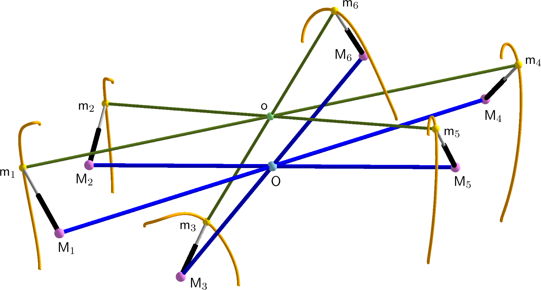
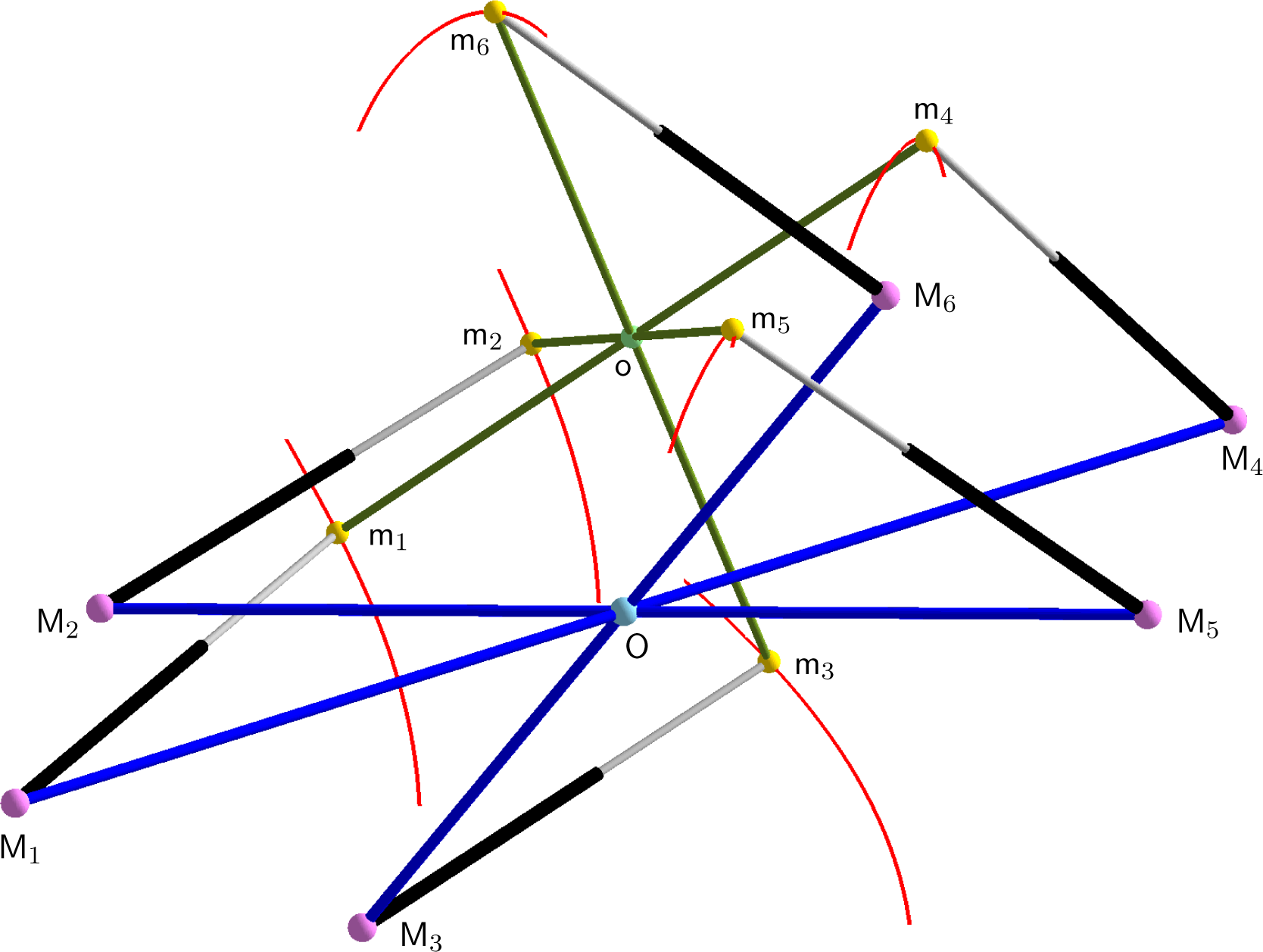
The geometry of a hexapod is given by the six base anchor points Mi with coordinates Mi := (Ai, Bi, Ci)T with respect to the fixed frame and by the six platform anchor points mi with coordinates mi := (ai, bi, ci)T with respect to the moving frame (for i = 1, …, 6). Each pair (Mi, mi) of corresponding anchor points of the fixed body Σ0 (base) and the moving body Σ (platform) is connected by an SPS-leg, where only the prismatic joint (P) is active and the spherical joints (S) are passive. Note that for a hexapod, (Mi, mi) ≠ (Mj, mj) holds for pairwise distinct i, j ∈ {1, …, 6}. Moreover, a hexapod is called planar, if M1, …, M6, as well as m1, …, m6 are coplanar; otherwise, it is called non-planar.
If the geometry of this so-called parallel manipulator of the Stewart–Gough type is given, as well as the lengths Ri ≥ 0 of the six legs, the hexapod is generically rigid. However, under particular conditions, this body-bar framework can perform an n-dimensional motion (n > 0), which is called self-motion (=continuous flexion).
Note that these overconstrained motions are also solutions to the still unsolved problem posed by the French Academy of Science for the “Prix Vaillant” of the year 1904, which is also known as the Borel–Bricard problem (cf. [1–3]) and reads as follows: “Determine and study all displacements of a rigid body in which distinct points of the body move on spherical paths.”
The necessary and sufficient condition for the infinitesimal flexibility of the hexapodal manipulator is that the carrier lines of the six legs belong to a linear line complex [4,5]. The corresponding configurations of the hexapod are called singular (or shaky). It is well known that hexapods, which are singular in every possible configuration, possess self-motions in each pose (over the field C of complex numbers). These so-called architecturally singular manipulators are well studied and classified (for the planar case, we refer to [6–9], and for the non-planar case, see [10,11]). In contrast, only a few self-motions of non-architecturally singular hexapods are known [12], as their computation is a very complicated task.
In this article, we study a special class of hexapods, which is defined as follows:
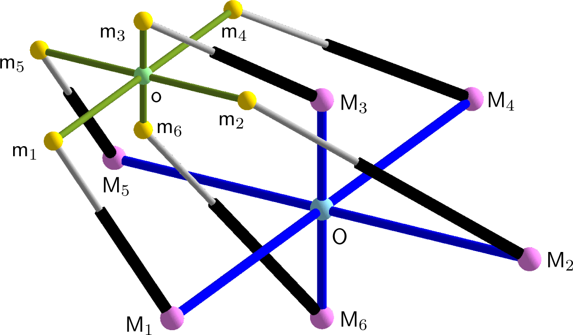
Definition 1. A hexapod is called point-symmetric if it has the following properties (after a possible necessary relabeling of anchor points):
- Mi and Mi+3 are symmetric with respect to a point O of the fixed frame for i = 1, 2, 3;
- mi and mi+3 are symmetric with respect to a point o of the moving frame for i = 1, 2, 3;
- None of the following three distance conditions are satisfied for all distinct i, j ∈ {1, 2, 3} : (a); (b); (c).
In the remainder of this article, we abbreviate “point-symmetric hexapod” as PSH. Item 3 of Definition 1 excludes trivial cases of architectural singularity; thus, only the following cases of architecturally singular PSHs remain:
Corollary 2. A PSH is architecturally singular if and only if one of the following cases hold (after a possible necessary renumbering of anchor points and the exchange of the platform and the base):
- m1, …, m6 are collinear;
- m1, m2, m4, m5 are collinear, M1, M2, M4, M5 are collinear and CR(m1, m2, m4, m5) = CR(M1, M2, M4, M5) holds, where CR denotes the cross-ratio;
- The platform and base are planar, and there exists a regular affinity with Mi ↦ mi for i = 1, …, 6.
Proof. The corollary can directly be concluded from the literature on architecturally singularity (see, e.g., Theorem 1 of [6] and Theorem 3 of [10]). □
Definition 3. A PSH is called orthogonal if it fulfills the following conditions:
- OM1, OM2, OM3 are pairwise orthogonal;
- om1, om2, om3 are pairwise orthogonal.
In the remainder of this article, we abbreviate “orthogonal PSH” as OPSH. An OPSH is illustrated in Figure 1. Moreover, note that an OPSH cannot be architecturally singular due to Corollary 2.
Remark 1. For better imagining the OPSH’s geometry (with for i = 1, 2, 3), the anchor points can be interpreted as the vertices of an ellipsoid in the fixed/moving space.
1.1. Results on OPSHs
Without loss of generality (w.l.o.g.), we can assume for any OPSH that M1 (resp. m1) is located on the x-axis, M2 (resp. m2) on the y-axis and M3 (resp. m3) on the z-axis of the fixed frame (resp. moving frame). Therefore, we get:
and
We can assume w.l.o.g. that A, a, B, b, C ≥ 0 holds, as the indices of the anchor points can be permuted and the role of the platform and the base can be exchanged.
Under the assumption that the local symmetry of the platform and the base is extended to the legs in the following way:
Dietmaier determined in Equation (13) of [13] the two necessary and sufficient conditions for the finite mobility of the OPSH. The first condition reads as follows:
and therefore, it only depends on the geometry of the OPSH. In the second equation, which is given by:
also the remaining free leg lengths R1, R2, R3 are involved. If these two conditions are fulfilled, the OPSH has a one-dimensional flexion, which we call the Dietmaier self-motion.
It can easily be checked that the two conditions given in Equations (6) and (7) are fulfilled independently of R1, R2, R3 if and only if A = a, B = b and C = c hold. As a consequence, there exists an orientation preserving congruence transformation τ with:
Therefore, hexapods, which possess this property, are called congruent.
All self-motions of congruent OPSHs were determined by Husty et al. in Example 3.3.8 of [14]. The following three types can be distinguished: two-dimensional translatoric self-motion, one-dimensional Schönflies self-motion and Dietmaier self-motion.
Remark 2. If τ of Equation (8) is an orientation reversing congruence transformation, we get a so-called reflection-congruent hexapod. In the more general case of τ being an equiform transformation, we name the hexapod an equiform one.
1.2. Outline of the Article
In Section 2, we give the basics of bond theory for hexapods and list some known results obtained by this method, including two corollaries for PSHs. After this preparatory work, we give in Section 3 necessary conditions for OPSHs in order to have a self-motion, which are also sufficient over ℂ.
In Section 4.1, we study the self-mobility of equiform PSHs in detail. Specifically, we classify all self-motions of congruent PSHs, which generalizes the above cited result of Husty et al. In Section 4.2, we determine a new set of PSHs with generalized Dietmaier self-motions.
We close the paper with some comments on the self-mobility of hexapods with global/local symmetries and list some open problems in this context, which are dedicated to future research.
2. Bond Theory
In this section, we give a short introduction to the theory of bonds presented in [15], which was motivated by the bond theory of overconstrained closed linkages with revolute joints given in [16]. We start with the direct kinematic problem of hexapods and proceed with the definition of bonds.
Due to the result of Husty [17], it is advantageous to work with Study parameters (e0 : e1 : e2 : e3 : f0 : f1 : f2 : f3) for solving the forward kinematics of hexapods. Note that the first four homogeneous coordinates (e0 : e1 : e2 : e3) are the so-called Euler parameters. Now, all real points of the Study parameter space P7 (seven-dimensional projective space), which are located on the so-called Study quadric
, correspond to an Euclidean displacement, with the exception of the three-dimensional subspace E of Ψ given by e0 = e1 = e2 = e3 = 0, as its points cannot fulfill the condition N ≠ 0 with
. The translation vector t := 2(t1, t2, t3)T and the rotation matrix R of the corresponding Euclidean displacement x ↦ Rx + t are given by:
and
if the normalizing condition N = 1 is fulfilled. All points of the complex extension of P7, which cannot fulfill this normalizing condition, are located on the so-called exceptional cone N = 0 with vertex E.
By using the Study parametrization of Euclidean displacements, the condition that the point mi is located on a sphere centered in Mi with radius Ri is a quadratic homogeneous equation according to Husty [17]. This so-called sphere condition Λi has the following form:
Now, the solution for the direct kinematics over C of a hexapod can be written as the algebraic variety V of the ideal spanned by Ψ, Λ1, …, Λ6, N = 1. In general, V consists of a discrete set of points, which correspond with the (at most) 40 solutions of the forward kinematic problem.
We consider the algebraic motion of the mechanism, which are the points on the Study quadric that the constraints define; i.e., the common points of the seven quadrics Ψ, Λ1, …, Λ6. If the manipulator has an n-dimensional self-motion, then the algebraic motion also has to be of this dimension. Now, the points of the algebraic motion with N ≠ 0 equal the kinematic image of V. However, we can also consider the points of the algebraic motion, which belong to the exceptional cone N = 0. An exact mathematical definition of these so-called bonds can be given as follows (cf. Remark 5 of [15]):
Definition 4. For a hexapod, the set of bonds is defined as:
where V* denotes the variety V after the removal of all components, which correspond to pure translational motions. Moreover ZarClo(V*) is the Zariski closure of V*, i.e., the zero locus of all algebraic equations that also vanish on V*.
The restriction to motions, which are not pure translations (=non-translational motions) is caused by the following approach used for the computation of bonds: in the first step, we project the algebraic motion of the hexapod into the Euler parameter space P3 by the elimination of f0,…,f3. This projection is denoted by πf. In the second step, we determine those points of the projected point set πf (V), which are located on the quadric N = 0; i.e.,
Note that this set of projected bonds, which is denoted by
, cannot be empty for a non-translational self-motion. Moreover, it is important to note that the set of bonds only depends on the geometry of the hexapod, and not on the leg lengths (cf. Theorem 1 of [15]).
Remark 3. A more sophisticated bond theory for pentapods and hexapods is based on a special compactification of SE(3), where the sphere condition Λi is only linear in 17 motion parameters. This approach, which was presented in [18], has many theoretical advantages compared to the method described above, but it is not suited for direct computations due to the large number of motion parameters. In contrast, the approach of the paper at hand was already successfully used for direct computations in [15,19–21].
Clearly, the kernel of this projection πf equals the group of translational motions. As a consequence, a component of V, which corresponds to a pure translational motion, is projected to a single point O (with N ≠ 0) of the Euler parameter space P3 by the elimination of f0, …, f3. Therefore, the intersection of O and N = 0 equals Ø, which warrants the exclusion of pure translational motions within this approach. However, this does not cause any trouble, as all hexapods with pure translational self-motion were already characterized by the author in [15] as follows:
A hexapod possesses a pure translational self-motion, if and only if the platform can be rotated about the center m1 = M1 into a pose, where the vectors
for i = 2, …, 6 fulfill the condition
. Moreover, all one-dimensional self-motions are circular translations, which can easily be seen by considering a normal projection of the manipulator in the direction of the parallel vectors
for i = 2, …, 6. If all of these six vectors are zero-vectors, which corresponds with the case that the platform and the base are congruent, we get the already mentioned two-dimensional translational self-motion of a hexapod (cf. [19]).
The above given characterization of hexapods with translational self-motions can be reformulated/tightened for PSH as follows:
Corollary 5. A PSH possesses a pure translational self-motion, if and only if the platform can be rotated about the center o = O into a pose, where the vectors for i = 1, 2, 3 fulfill the condition.
Proof. The proof follows directly from the fact that the midpoint property is invariant under parallel projections. □
Moreover, we have the following result on multidimensional self-motions of PSHs:
Corollary 6. A non-architecturally singular PSH can only have an n-dimensional self-motion with n > 1 if it is congruent. The self-motion is the two-dimensional translation.
3. OPSH With Self-Motions
Due to the above outlined computational approach of bonds, we divide the discussion of self-motions into two sections; namely translational and non-translational ones.
3.1. Necessary Condition for Translational Self-Motions
Based on Corollary 5, the following statement can be proven for OPSH:
Theorem 7. A pure translational self-motion of an OPSH can only exist in one of the following five cases:
Therefore, a necessary condition on the geometry is that holds for at least one i ∈ {1, 2, 3}.
Proof. Due to Corollary 5, we compute the vectors
by Rmi − NMi and express the condition for their linear dependency by Kk = o, where o denotes the zero-vector and Kk is given by:
for pairwise distinct i, j, k ∈ {1, 2, 3}. We denote the condition implied by the first, second and third line of Kk = o by
and
, respectively. Therefore, we have to show that this resulting system of nine equations
can only be fulfilled in one of the five cases α, …, ε. This can be done as follows:
Due to item 3(c) of Definition 1, we can assume that abc ≠ 0 (after a maybe necessary exchange of the platform and the base). Therefore, we can cancel the factors 2aN from
and
, 2bN from
and
, 2cN from
and
and only N from
,
and
, respectively. We denote the remaining expressions by
. Then, we consider the following linear combinations:
As a, b > 0 and A, B ≥ 0 holds w1 and w4 can only be fulfilled in the following two cases:
- e1 = e2 = 0: Then, w6 is either fulfilled for c = C (⇒ case γ) or for:
- e0 = 0: We get , which cannot vanish without contradiction (w.c.).
- e3 = 0: In this case, we get:Therefore, a = A (⇒ case α), b = B (⇒ case β) or c = C (⇒ case γ) has to hold.
- e3 = 0: For the discussion of this case, we can assume that e1 = e2 = 0 does not hold. We distinguish the following cases:
- e1e2 ≠ 0: Under this assumption, w5 yields c = −C. Then, we get:which implies either e0 = 0 (⇒ case δ) or the reflection-congruent OPSH (⇒ case ε).
- e1 = 0, e2 ≠ 0: Now, w3 can only vanish either for b = B (⇒ case β) or e0 = 0. In the latter case, we get , which also implies b = B (⇒ case β).
- e2 = 0, e1 ≠ 0: This case can be discussed analogously to the last one, with the sole exception that we always end up in the case α.
We close this subsection by giving some comments on the cases α, …, ε:
Note that the conditions given in the cases α, …, δ are not sufficient for the existence of a real translational self-motion, as in each case, one homogeneous quadratic equation in two Euler parameters remains, which may have complex solutions. In the case of a real solution, the loop Mi, mi, mi+3, Mi+3 forms a parallelogram during the translatoric self-motion of case α (i = 1), β (i = 2), γ (i = 3) and δ (i = 3).
Contrary, in case ε, we get for each orientation of the two-dimensional set determined by e3 = 0, a real translatoric self-motion. For more details on this reflection-congruent case, we refer to [20].
Finally, it should again be noted that all translational self-motions are one-parametric circular translations with the exception of the congruent OPSH, which has a two-dimensional translatoric mobility. Note that the congruent OPSH belongs to all three cases α, β, γ simultaneously.
3.2. Necessary Condition for Non-Translational Self-Motions
Within this section, we prove the following main theorem:
Theorem 8. An OPSH can have a non-translational self-motion only if either Equation (6) is fulfilled or abcABC = 0 holds.
Proof. The proof of this theorem is done by the bond theory presented in Section 2; i.e., we determine the conditions for the existence of a projected bond. For the computational proof, we need the two linear combinations:
which read in detail as follows:
Note that G1 and G2 do not depend on f0, f1, f2, f3. Besides these two expressions, also the following three equations:
are of interest, as they are linear in f0, f1, f2, f3. Now, we split the proof up into a general case and a special one.
General case: For this case, we assume that ν ≠ 0 holds, where ν is given by:
Under this assumption, we can solve the system Ψ, Δ1,4, Δ2,5, Δ3,6, which is linear in f0, f1, f2, f3 for these variables. Plugging the obtained expressions in Λ1, we obtain in the numerator the expression NG0[5064], where G0 is homogeneous of degree six in the Euler parameters. Note that the number in the brackets gives the number of terms.
Therefore, a real self-motion can only exist if the sextic surface G0 = 0 and the two quadrics G1 = G2 = 0 have a curve in common. If this is the case, there also has to exist at least one intersection point (projected bond) of this curve with the exceptional quadric N = 0.
In the next step, we eliminate e0 by computing the resultant Hi of Gi and N for i = 0, 1, 2. We get:
Now, we proceed with the elimination procedure by calculating the resultant Lk of Hi and Hj for pairwise distinct i, j, k ∈ {0, 1, 2}. Then, we eliminate e1 by computing the resultant Qk of Li and Lj for pairwise distinct i, j, k ∈ {0, 1, 2}. Now, the necessary condition for the existence of a projected bond is that the greatest common divisor of Q0, Q1, Q2 vanishes, which reads as follows (up to powers of the given factors):
As the back-substitution of e2 = 0 implies e1 = e3 = e0 = 0 (a contradiction), the theorem is proven for the general case.
Special case: Now, we consider the special case ν = 0. Therefore, we have to determine the condition for the existence of a common point of the four quadrics G1 = G2 = ν = N = 0.
If we replace G0 by ν, the same elimination procedure as in the general case yields the following greatest common divisor (up to powers of the given factors) of the resulting final expressions:
As the back-substitution of e2 = 0 implies again e1= e3 = e0 = 0 (a contradiction), the theorem is proven. □
Remark 4. A consequence of the Theorems 7 and 8 is that an OPSH with for i = 1, 2, 3, which does not fulfill Equation (6), is free of self-motions. This is of importance for practical applications, as self-motions are dangerous, because they are uncontrollable and, thus, a hazard to man and machine. Therefore, being able to avoid OPSH designs that engender self-motion is of interest to engineers. Note that also the later given Theorem 4.1 should be read in this context.
Note that the condition abcABC = 0 is even sufficient for the existence of a real self-motion due to the following two examples. For the description of these trivial examples, we can assume (after a maybe necessary relabeling of anchor points and an exchange of platform and base) that a = 0 holds; i.e., m1 = m4 = o:
- Butterfly self-motions: If the platform is located in a way that the y-axis (z-axis) of the moving frame coincides with the z-axis (y-axis) of the fixed frame, then the platform can rotate freely around this line.
- Spherical four-bar self-motion: If the platform is in a configuration where the centers of the moving frame and fixed frame coincide (⇔ o = O), then the manipulator can perform a spherical four-bar motion with center o = O.
If the condition given in Equation (6) is fulfilled, we will see later on (cf. Theorem 12 under consideration of Remark 7) that this is already sufficient for the existence of a self-motion over ℂ, namely a Dietmaier self-motion. In the following, we want to take a closer look at the Dietmaier self-motion, in order to clarify the algebraic reasoning for this mobility.
3.2.1. Dietmaier Self-Motions
Under the assumption that the leg lengths fulfill Equation (5), the equations Δ1,4, Δ2,5, Δ3,6 are homogeneous linear equations in f0, …, f3. Therefore, we distinguish the following two cases:
ν ≠ 0: In this case, we can solve Ψ, Δ1,4, Δ2,5, Δ3,6 for f0, …, f3, which yields f0 = f1 = f2 = f3 = 0. As a consequence, we can only have a pure spherical self-motion, as o = O holds.
By projecting the OPSH onto a sphere centered in o = O and identifying antipodal points, we get a three-legged spherical three-dof RPR manipulator if abcABC ≠ 0 holds. Due to Theorem 6 of [15], it is known that such a spherical mechanism can only have a self-motion if two platform or base anchor points coincide, which cannot be the case, due to the underlying OPSH structure. Therefore, abcABC = 0 has to hold, and we get the above mentioned trivial solution of spherical four-bar self-motions (including special butterfly self-motions). Note that these are not Dietmaier self-motions, as for abcABC = 0, the condition given in Equation (6) cannot be fulfilled without contradiction over ℝ.
ν = 0: The above study shows that ν = 0 has to hold for a Dietmaier self-motion. Note that ν = G1 = G2 = 0 are three homogeneous quadratic equations in the Euler parameters without mixed terms eiej for i 6= j ∈ {0, …, 3}. Under the Dietmaier conditions given in Equations (6) and (7), the three quadrics in the Euler parameter space are linearly dependent, which is already sufficient for the existence of a self-motion over ℂ. Based on this observation, we will determine a new set of PSH with non-translatoric self-motions in Section 4.2.
Example 1. For a detailed example of a Dietmaier self-motion, please see [13]. We only want to note in this context an example with rational coordinates fulfilling Equation (6):
Remark 5. It is still an open problem to determine all non-translational self-motions of an OPSH besides the known Dietmaier self-motion, spherical four-bar self-motion and the butterfly self-motion. It is only known (cf. last paragraph of Section 1.1) that congruent OPSHs also have Schönflies self-motions.
In this context, it should finally be noted that equiform OPSHs, which are not congruent, cannot possess non-translational self-motions, as Equation (6) has no solution over R. We will generalize this result in the next section.
4. PSHs with Self-Motions
The geometric characterization of PSHs with translational self-motions was already done in Corollary 5. Therefore, we focus on conditions for non-translational self-motions, where trivial examples are again the butterfly self-motion (which exists if four anchor points are collinear) and the spherical four-bar self-motion (which exists if
or
holds). The procedure for the computation of such necessary conditions is the same as the one given in the proof of Theorem 8, but due to the number of involved variables and the resulting lengths and degrees of the obtained equations, the author failed to compute the final expressions Q0, Q1, Q2 running Maple 17 on a computer with 12 GB RAM (not even for planar PSHs). Therefore, we restrict ourselves to equiform/congruent PSHs, which are studied next.
4.1. Equiform/Congruent PSHs
Theorem 9. If an equiform PSH has a non-translational self-motion, then it is either congruent or architecturally singular.
Proof. W.l.o.g., we can choose coordinate systems in the platform and the base in a way that we have:
for i = 1, 2, 3 with b1 = c1 = c2 = B1 = C1 = C2 = 0 and the remaining coordinates are coupled by:
where μ ≠ 0 is the similarity factor.
We proceed with analogous computations as in the proof of Theorem 8, but now, ν is given by:
For the general case (ν ≠ 0), we end up with the following necessary condition:
μA1 = 0 contradicts the definition of a PSH, and B2 = 0 results in an architecturally singular design (cf. Item 2 of Corollary 2). Moreover,
implies B3 = C3 = 0, and we get again Item 2 of Corollary 2. The last factor can only be fulfilled for C3 = 0 and A2B3 − A3B2 = 0, which also implies Item 2 of Corollary 2.
For the special case (ν = 0), we end up with the following necessary condition:
with
μA1 = 0 contradicts the definition of a PSH, μ = 1 yields a congruent PSH and B2 = 0 results in Item 2 of Corollary 2. Therefore, we can assume B2 ≠ 0, which implies that Fi can only be fulfilled over ℝ for C3 = 0 for i = 1, 2, 3, 4. Therefore, C3 = 0 has to hold, which implies a planar equiform hexapod. These manipulators were already studied in detail in [23,24] with the result that they cannot have self-motions if they are not architecturally singular. This closes the proof of the theorem. □
In the context with Theorem 9, it should be noted that equiform hexapods have a translational self-motion if and only if they are reflection congruent or congruent (cf. [20]). In the latter case, we get the already mentioned two-dimensional translation. The non-translational self-motions of congruent PSHs, which were excluded from Theorem 9, are the content of the next theorem, which generalizes the result of Husty et al., mentioned at the end of Section 1.1. For the formulation of this theorem, the following definition is needed:
Definition 10. A self-motion of a PSH is called generalized Dietmaier self-motion, if Equation (5) holds and the equations Ψ, Δ1,4, Δ2,5, Δ3,6 are linearly dependent with respect to f0, …, f3.
Theorem 11. A congruent PSH, which is not architecturally singular, can have the following two types of non-translation self-motions:
- Line-symmetric self-motions (including Schönflies self-motions as a special case),
- Generalized Dietmaier self-motions.
Proof. We use the same coordinatization as in the proof of Theorem 9 under consideration of μ = 1. Moreover, we can assume that the congruent PSH is non-planar, because it is well-known (cf. [24]) that planar ones can only have translational self-motions, if they are not architecturally singular.
Within the proof, we distinguish the following two cases:
- e3 ≠ 0: Under this assumption, we can solve Ψ, Δ1,4, Δ2,5 for f1, f2, f3. Plugging the obtained expressions into Δ3,6 yields in the numerator with:Therefore, E = 0 has to hold. Beside this condition, we have again the linear combinations G1 and G2 of Equation (20), which now read as follows:The last remaining condition results from Λ1 after plugging the expressions for f1, f2, f3 into it. However, this condition is not of interest, as one can always solve it for f0 in case of a non-translational self-motion. Therefore, the two quadrics G1 = G2 = 0 and the plane E = 0 in the Euler parameter space have to have a curve s in common. We distinguish the following cases:
- E = 0 is not fulfilled identically: In this case, we consider the expression of E after replacing ei by fi for i = 1, 2, 3. This yields:If we plug the obtained solutions for f1, f2, f3 into F, the numerator factors into two factors, where one of it is E. Therefore, E = 0 implies F = 0; thus, we have two linear relations between the Study parameters. According to [25], this is one possible characterization of line-symmetric motions. In general, the curve s is a regular conic section, but it can also happen that it consists of one or two straight lines, implying Schönflies self-motions.Remark 6. Note that the geometric characterization of parallel manipulators with a Schönflies self-motion was already done in [26], and therefore, this case can only be a special case of it.
- E = 0 is fulfilled identically: As A1B2C3 ≠ 0 holds, this can only be the case if Equation (5) holds. Therefore, we get a generalized Dietmaier self-motion, which corresponds in the generic case with a curve s of degree four in the Euler parameter space.
- e3 = 0: Now, Δ1,4 and Δ2,5 do not depend on f0, f1, f2. Elimination of f3 implies that E = 0 has to hold with:If E = 0 is not fulfilled identically, it already determines a straight line in the Euler parameter space, and therefore, we can only end up with a Schönflies self-motion.For R1 = R4 and R2 = R5, the equation E = 0 is fulfilled identically. Now, Δ1,4 and Δ2,5 can only vanish without contradiction for f3 = 0. Due to e3 = f3 = 0, we can only end up with a line-symmetric self-motion.
Example 2. We give an example of a line-symmetric self-motion, which is not a Schönflies motion, as this is the essential new possibility compared to the classification of congruent OPSHs. The geometry is given by:
We can compute f1, f2, f3 from Ψ, Δ1,4, Δ2,5. Moreover, for the choice:
we get from the condition E = 0. Now, G2 is a real-valued multiple of G1, which determines the conic s (and therefore, the self-motion) by the equation:
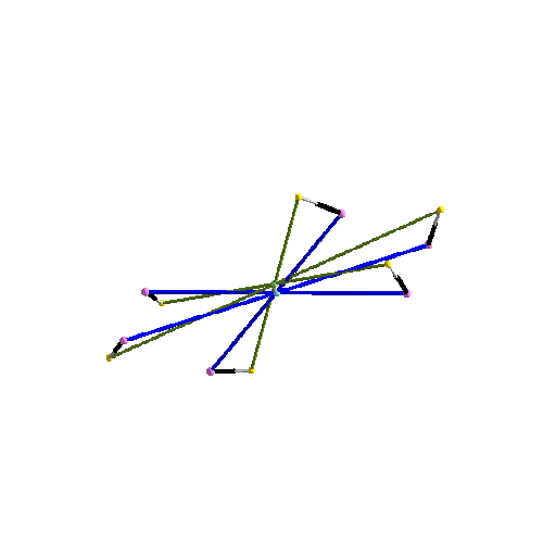
This equation can be solved for e0 and plugged into Λ1. As this final equation is quadratic in f0, the self-motion is in general not rational.
A real line-symmetric self-motion (cf. Figure 2) is, for example, obtained for the following values: For,
,
and e3 = 1, the self-motion is real if e2 is within the interval [−t, t] with:
4.2. Generalized Dietmaier Self-Motions
In this section, we want to determine further PSHs (beside congruent PSHs), which have generalized Dietmaier self-motions. Under the assumption of Equation (5), we see that the equations Δ1,4, Δ2,5, Δ3,6 are homogeneous linear in f0, …, f3. Therefore, a necessary and sufficient condition for a generalized Dietmaier self-motion is that the three quadrics G1 = G2 = ν = 0 in the Euler parameter space have a curve in common, where G1 and G2 are defined as in Equation (20) and ν is the remaining factor of the determinant of the coefficient matrix of Ψ, Δ1,4, Δ2,5, Δ3,6 with respect to f0, …, f3 after splitting away N.
W.l.o.g., we can assume coordinate systems in the platform and the base in a way that o and O, respectively, are their origins, m1 and M1 are on their x-axes and m2 and M2 are located in their xy-planes, which implies:
for i = 1, 2, 3. With respect to these coordinate systems, the three equations have the following numbers of terms: G1[48], G2[68], ν[64]. The resultant of each of these two equations with respect to any Euler parameter is a quartic in the remaining ones with more than 20,000 terms. Therefore, the author was not able to compute the general conditions for the existence of a common curve s of G1 = G2 = ν = 0 (as the calculation of the resultant of two such quartics failed by Maple 17 on a computer with 12 GB RAM).
Therefore, we restrict to the following case: The quadrics G1 = G2 = ν = 0 are linearly dependent as for the original Dietmaier self-motion (cf. Section 3.2.1); i.e., there exists a linear combination:
As a consequence, the curve s in the Euler parameter space is of degree four.
Theorem 12. The following set D of non-architecturally singular PSHs with non-planar platform and non-planar base has a generalized Dietmaier self-motion:
and the following condition remains with:
with respect to the coordinate systems of Equation (50). Therefore,
is a seven-dimensional set of PSHs (excl. similarities), where each design possesses at least a two-parametric set of generalized Dietmaier self-motions over. Only in the case of congruence we get a three-parametric set of generalized Dietmaier self-motions.
Proof. Due to the non-planarity assumption of the platform and the base, we can assume a1A1b2B2c3C3 6= 0. Moreover, we can even assume w.l.o.g. that a1, A1, b2, B2 > 0 holds.
For the computational proof, we denote the coefficient of
of L by Lijkl. Then, we consider the following set of 10 necessary and sufficient equations:
In detail, these equations read as follows:
Note that only the equation w1 depends on the leg lengths R1, R2, R3. W.l.o.g., we can solve w2, w3 for λ1 and λ2. As λ = 0 implies λ1 = λ2 = 0 a contradiction, we can set λ = 1. Then, w5 implies b3 of Equation (52), and w8 can only vanish w.c. for:
Then, w9 implies a2 of Equation (52). Substituting this expression into Equation (56) yields the condition for a3 given in Equation (52). Now, one condition on the geometry of the PSH remains, namely w3, which is the equation given in Equation (53).
Remark 7. Note that w3 implies the condition of Equation (6) under the additional assumption A2 = A3 = B3 = 0 of an OPSH. Note that therefore the original Dietmaier self-motion is included as a special case.
Besides this condition, only w1 is not fulfilled, which has the following structure:
. Therefore, each design of D has at least a two-parametric set of generalized Dietmaier self-motions. We only get a three-parametric set if this linear relation in
,
and
is fulfilled identically, which is studied next.
The condition q3 = 0 implies
. Then, q2 can only vanish w.c. for a1 = A1. Now, q1 = 0 is already fulfilled identically, and we remain with the conditions w3 and q0 = 0. It can easily be seen that w3 implies b2 = B2; i.e., the congruent PSH. Now, q0 = 0 is also fulfilled identically. □
Remark 8. Finally, it should be noted that a geometric interpretation of the algebraic conditions determining the set D is missing. This also includes the geometric meaning of Equation (6) (cf. Remark 7).
Based on the set of equations w1, …, w10 used in the proof of Theorem 12, it can be shown by a straightforward discussion of cases that a linear combination of Equation (51) does not exist for non-architecturally singular PSHs, if the platform or the base or both are planar. Therefore, the only missing cases yielding a generalized Dietmaier self-motion are those where s is a cubic curve, a conic section or a straight line in the Euler parameter space. The latter case is of less interest, as it can only be a special case of the manipulators given in [26] (cf. Remark 6).
Example 3. In the following, we give an example for a generalized Dietmaier self-motion. The PSH of the set D is given by:
Under consideration of Equation (5), the leg lengths are determined by:
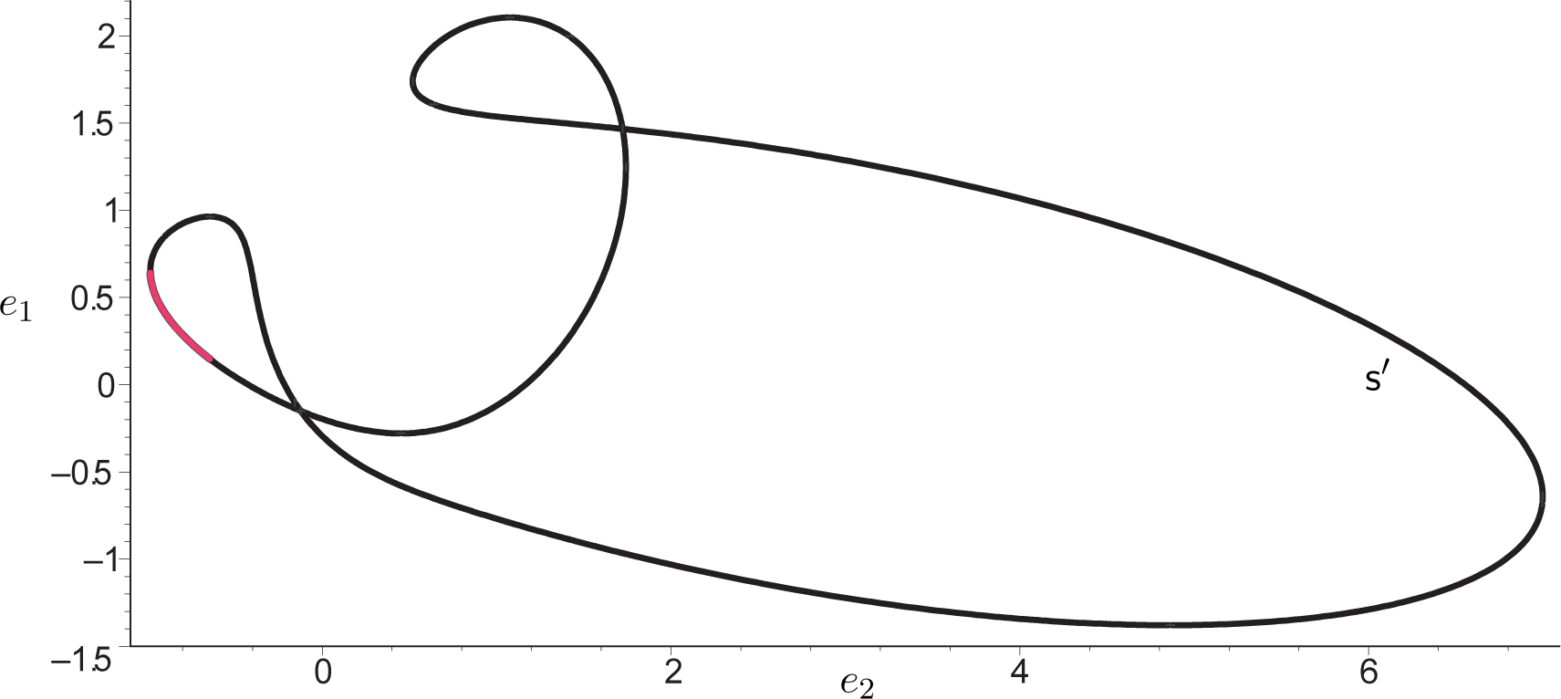
The projection of the quartic curve s in the Euler parameter space onto the e1e2e3-plane by the elimination of e0 yields the planar quartic curve s′ given by:
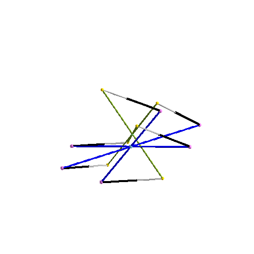
which is illustrated in Figure 3. The red plotted part of s′ corresponds with the real self-motion illustrated in Figure 4.
5. Conclusions and Future Work
We formulated necessary conditions for the geometry of OPSHs in order to possess a self-motion (cf. Theorems 7 and 8). Moreover, these conditions are also sufficient for the existence of such motions over ℂ. We also gave a full discussion of self-motions of equiform/congruent PSHs, which are not architecturally singular (cf. Section 4.1). Due to the large number of unknowns, a classification of general PSHs with self-motions remains open. Even though not all PSHs with a generalized Dietmaier self-motion (cf. Definition 10) could be determined, we were able to solve the most general case of generalized Dietmaier self-motions (cf. Theorem 12), which implies new solutions to the more than 100-year-old Borel–Bricard problem.
This study also shows that even for PSHs, which have a simplified geometry due to the symmetry assumptions, the computation of self-motions remains a very challenging/complicated task. This gives us just an idea of the complexity of the still open Borel–Bricard problem.
5.1. Hexapodal Self-Motions Viewed under the Aspect of Symmetry
One can think of other local symmetries in the platform and the base, respectively, besides the point-symmetry studied within this article; e.g., line-symmetry, plane-symmetry, 120°-rotational symmetry, etc. Results on self-motions of equiform/congruent plane-symmetric hexapods were already given in [19,20], respectively. Moreover, a full discussion of self-motions of the original Stewart–Gough hexapod (the platform and base both have a 120°-rotational symmetry) was given by Karger and Husty in [27]. Clearly, one can also study hexapods with mixed local symmetries; e.g., the platform is point-symmetric and the base is plane-symmetric. The self-mobility of hexapods with local symmetries is dedicated to future research.
Obviously, the local symmetries in the platform and base are preserved under a self-motion. However, there also exist hexapods with self-motions, which preserve the global symmetry of the hexapod. Examples for this phenomenon are the Bricard octahedra of Type 1 (=line-symmetric octahedron) and Type 2 (=plane-symmetric octahedron; see, e.g., [28]), respectively, as they can also be seen as hexapods.
A generalization of the self-motions of Type 1 Bricard octahedra was obtained by the author in [29]. These planar hexapods with so-called Type 2 DM (=Darboux–Mannheim) self-motions do not possess the global symmetry property any longer, but their self-motions are still line-symmetric ones (cf. [25]). In this context, it should finally be noted that most of the known hexapodal self-motions (cf. [12]) are line-symmetric motions.
Acknowledgments
This research is funded by Grant No. P 24927-N25 of the Austrian Science Fund FWF within the project “Stewart–Gough platforms with self-motions”.
Conflicts of Interest
The author declares no conflict of interest.
References
- Borel, E. Mémoire sur les déplacements à trajectoires sphériques. In Mém. Présent. Var. Sci. Acad. Sci. Natl. Inst. Fr. TOME XXXIII; Imprimerie Nationale: Paris, France, 1908; pp. 1–128. [Google Scholar]
- Bricard, R. Mémoire sur les déplacements à trajectoires sphériques. J. École Polytech. 1906, 11, 1–96. [Google Scholar]
- Husty, M.; Borel’s, E.; Bricard’s, R. Papers on Displacements with Spherical Paths and their Relevance to Self-Motions of Parallel Manipulators, Proceedings of the International Symposium on History of Machines and Mechanisms—HMM 2000, Cassino, Italy, 11–13 May 2000; Ceccarelli, M., Ed.; Kluwer: Dordrecht, The Netherlands, 2000; pp. 163–171.
- Merlet, J.-P. Singular configurations of parallel manipulators and Grassmann geometry. Int. J. Robot. Res. 1992, 8, 45–56. [Google Scholar]
- Pottmann, H.; Wallner, J. Computational Line Geometry; Springer: Berlin/Heidelberg, Germany, 2001. [Google Scholar]
- Karger, A. Architecture singular planar parallel manipulators. Mech. Mach. Theory 2003, 38, 1149–1164. [Google Scholar]
- Nawratil, G. On the degenerated cases of architecturally singular planar parallel manipulators. J. Geom. Graph. 2008, 12, 141–149. [Google Scholar]
- Röschel, O.; Mick, S. Characterisation of architecturally shaky platforms. In Advances in Robot Kinematics: Analysis and Control; Lenarcic, J., Husty, M.L., Eds.; Kluwer: Dordrecht, The Netherlands, 1998; pp. 465–474. [Google Scholar]
- Wohlhart, K. From higher degrees of shakiness to mobility. Mech. Mach. Theory 2010, 45, 467–476. [Google Scholar]
- Karger, A. Architecturally singular non-planar parallel manipulators. Mech. Mach. Theory 2008, 43, 335–346. [Google Scholar]
- Nawratil, G. A New Approach to the Classification of Architecturally Singular Parallel Manipulators. In Computational Kinematics; Kecskemethy, A., Müller, A., Eds.; Springer: Berlin/Heidelberg, Germany, 2009; pp. 349–358. [Google Scholar]
- Nawratil, G. Review and recent results on Stewart Gough platforms with self-motions. Appl. Mech. Mater. 2012, 162, 151–160. [Google Scholar]
- Dietmaier, P. Forward kinematics and mobility criteria of one type of symmetric Stewart-Gough platforms. In Recent Advances in Robot Kinematics; Lenarcic, J., Parenti-Castelli, V., Eds.; Kluwer: Dordrecht, The Netherlands, 1996; pp. 379–388. [Google Scholar]
- Husty, M.; Karger, A.; Sachs, H.; Steinhilper, W. Kinematik und Robotik; Springer: Berlin/Heidelberg, Germany, 1997. [Google Scholar]
- Nawratil, G. Introducing the theory of bonds for Stewart Gough platforms with self-motions. ASME J. Mech. Rob. 2014, 6. [Google Scholar] [CrossRef]
- Hegedüs, G.; Schicho, J.; Schröcker, H.-P. Bond Theory and Closed 5R Linkages. In Latest Advances in Robot Kinematics; Lenarcic, J., Husty, M., Eds.; Springer: Berlin/Heidelberg, Germany, 2012; pp. 221–228. [Google Scholar]
- Husty, M.L. An algorithm for solving the direct kinematics of general Stewart–Gough platforms. Mech. Mach. Theory 1996, 31, 365–380. [Google Scholar]
- Gallet, M.; Nawratil, G.; Schicho, J. Bond theory for pentapods and hexapods. J. Geom. 2014. [Google Scholar] [CrossRef]
- Nawratil, G. Congruent Stewart Gough platforms with non-translational self-motions. Proceedings of the 16th International Conference on Geometry and Graphics, Innsbruck, Austria, 4–8 August 2014; pp. 204–215.
- Nawratil, G. On equiform Stewart Gough platforms with self-motions. J. Geom. Graph. 2013, 17, 163–175. [Google Scholar]
- Nawratil, G. On Stewart Gough manipulators with multidimensional self-motions. Comput. Aided Geom. Des. 2014, 31, 582–594. [Google Scholar]
- Nawratil, G.; Schicho, J. Pentapods with Mobility 2. ASME J. Mech. Rob. 2014. [Google Scholar] [CrossRef]
- Karger, A. Singularities and self-motions of equiform platforms. Mech. Mach. Theory 2001, 36, 801–815. [Google Scholar]
- Nawratil, G. Self-motions of planar projective Stewart Gough platforms. In Latest Advances in Robot Kinematics; Lenarcic, J., Husty, M., Eds.; Springer: Berlin/Heidelberg, Germany, 2012; pp. 27–34. [Google Scholar]
- Selig, J.M.; Husty, M. Half-turns and line symmetric motions. Mech. Mach. Theory 2011, 46, 156–167. [Google Scholar]
- Husty, M.L.; Karger, A. Self motions of Stewart-Gough platforms, an overview. Proceedings of the Workshop on Fundamental Issues and Future Research Directions for Parallel Mechanisms and Manipulators, Quebec City, Canada, 2–3 October 2002; pp. 131–141.
- Karger, A.; Husty, M. Classification of all self-motions of the original Stewart–Gough platform. Comput. Aided Des. 1998, 30, 205–215. [Google Scholar]
- Stachel, H. On the flexibility and symmetry of overconstrained mechanisms. Phil. Trans. R. Soc. A 2014, 372. [Google Scholar] [CrossRef]
- Nawratil, G. Planar Stewart Gough platforms with a type II DM self-motion. J. Geom. 2011, 102, 149–169. [Google Scholar]
Figure 1.
Sketch of a so-called orthogonal point symmetric hexapod (OPSH).

Figure 2.
The trajectories of the platform anchor points under (one branch of) the line-symmetric self-motion of Example 2 are displayed. An animation of this motion is provided as supplementary data (see Supplementary File S1).
Figure 2.
The trajectories of the platform anchor points under (one branch of) the line-symmetric self-motion of Example 2 are displayed. An animation of this motion is provided as supplementary data (see Supplementary File S1).

Figure 3.
We identify e3 = 0 with the line at infinity and illustrate the affine part of the planar quartic s′; i.e., we set e3 = 1 and plot e2 horizontally and e1 vertically.
Figure 3.
We identify e3 = 0 with the line at infinity and illustrate the affine part of the planar quartic s′; i.e., we set e3 = 1 and plot e2 horizontally and e1 vertically.

Figure 4.
The trajectories of the platform anchor points under a part of the self-motion of Example 3 are displayed. An animation of this motion is provided as supplementary data (see Supplementary File S2).
Figure 4.
The trajectories of the platform anchor points under a part of the self-motion of Example 3 are displayed. An animation of this motion is provided as supplementary data (see Supplementary File S2).

© 2014 by the authors; licensee MDPI, Basel, Switzerland This article is an open access article distributed under the terms and conditions of the Creative Commons Attribution license (http://creativecommons.org/licenses/by/4.0/).
Share and Cite
MDPI and ACS Style
Nawratil, G. On the Self-Mobility of Point-Symmetric Hexapods. Symmetry 2014, 6, 954-974. https://doi.org/10.3390/sym6040954
AMA Style
Nawratil G. On the Self-Mobility of Point-Symmetric Hexapods. Symmetry. 2014; 6(4):954-974. https://doi.org/10.3390/sym6040954
Chicago/Turabian StyleNawratil, Georg. 2014. "On the Self-Mobility of Point-Symmetric Hexapods" Symmetry 6, no. 4: 954-974. https://doi.org/10.3390/sym6040954