
Crystallography and Magnetic Phenomena

Abstract
: This essay describes the development of groups used for the specification of symmetries from ordinary and magnetic point groups to Fedorov and magnetic space groups, as well as other varieties of groups useful in the study of symmetric objects. In particular, we consider the problem of some incorrectness in Vol. A of the International Tables for Crystallography. Some results of tensor calculus are presented in connection with magnetoelectric phenomena, where we demonstrate the use of Ascher’s trinities and Opechowski’s magic relations and their connection. Specific tensor decomposition calculations on the grounds of Clebsch Gordan products are illustrated.1. Magnetism
Magnetism is a class of physical phenomena that includes forces exerted by magnets on other magnets or objects able to be magnetized. It was known by its effect in historical times; the Chinese knew about the compass a long time before Europeans. The magnetic compass was first invented as a device for divination as early as the Chinese Han Dynasty (about 206 BC) and in Song Dynasty China by the military for navigational orienteering by 1040–1044 AD, and it was used for maritime navigation by 1111 to 1117 AD. The first use of a compass is recorded in Western Europe between 1187 and 1202 AD and in Persia in 1232 AD. The dry compass was invented in Europe around 1300 AD. This was supplanted in the early 20th century by the liquid-filled magnetic compass.
The origin of magnetization is in electric currents and the fundamental magnetic moments of certain atoms. These give rise to a magnetic field that acts on other currents and moments. All materials are influenced to some extent by a magnetic field, and we distinguish the following types of magnetic materials: diamagnetic, paramagnetic, ferromagnetic, antiferromagnetic and various types of ordered magnetic materials.
Diamagnetism is caused by the precession of electrons in their orbits, when an external magnetic field is applied. Diamagnetism is therefore always present if not obscured by a stronger field. It appears as a reaction of the external field in any material and is very low.
Paramagnetism is due to the material’s own magnetic moments of its atoms, which attempt to align in the direction of an external magnetic field. The ions or atoms in these materials interact very slightly, and this interaction competes with thermal motion.
Ferromagnetism is the strongest of magnetisms, and it keeps its magnetized state even after the external field is removed. The atoms of these substances have unpaired electrons in the 4d orbitals of iron or 4f (and 5d) in lanthanides. Thus, we observe ferromagnetism in Fe, Ni, Co, Gd, their different alloys and in alloys that do not even contain ferromagnetic elements, like Heusler alloys of Mn, Sn, Al, Bi and B, while As, Sb, Bi, B and Cu are even themselves diamagnetic.
The strong attraction of moments is due to the so-called Weiss field, which later was explained by Frenkel and Heisenberg.
Magnetic oxides are relatively new materials (20th century) in which we can observe various types of magnetic ordering. If the paramagnetic atoms are incorporated in a crystal lattice, they are subject to an internal field (Weiss field), which can force the elementary magnets to align either parallel (ferro) or antiparallel (antiferro or ferri).
Most magnetic oxides are based on a substructure of closely-packed oxygen atoms. The close packing results either in a cubic (spinel and garnet) or in a set of hexagonal arrangements (magnetoplumbite or hexagonal ferrites), which depend on the sequence of oxygen layers. The cubic structure (spinel) contains two tetrahedral sites of opposite orientations and one octahedral site per unit cell. Spinel (MgAl3O4) and garnet (Mn3Al2(SiO4)3) are precious stones, and industrial compounds contain some paramagnetic atoms in the place of Mg, Mn or Al.
In Figure 1, we show the antiferromagnetic ordering of Co in CoO, where the magnetic unit cell has twice as large edges as the non-magnetic cell.
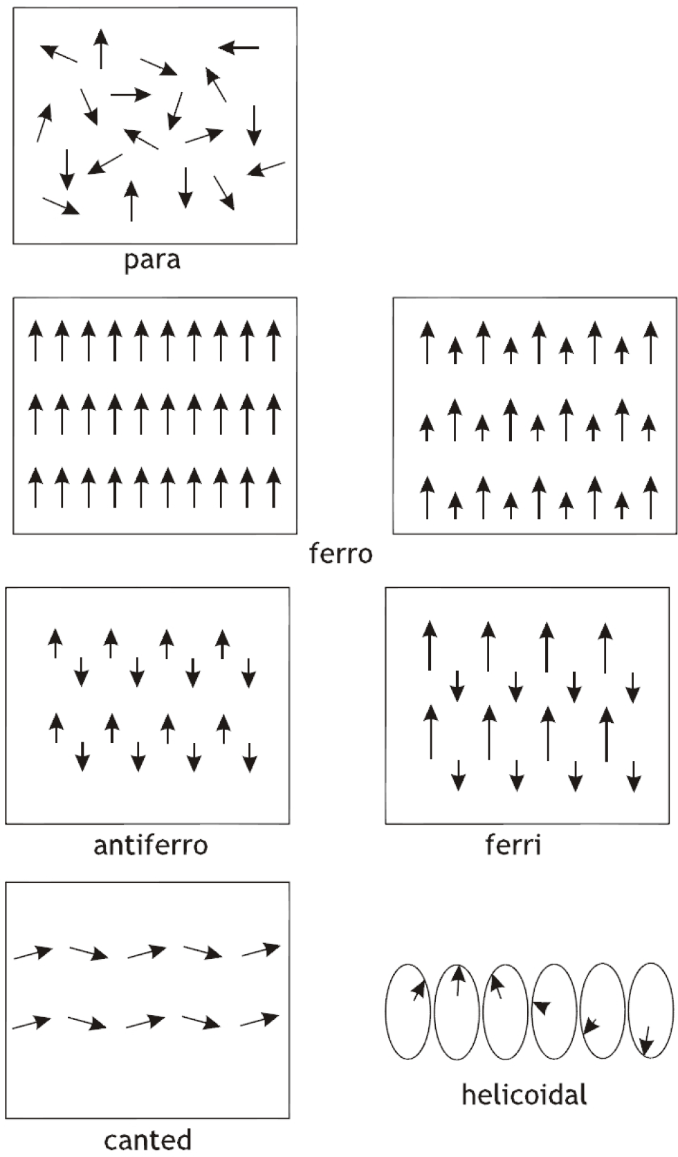
More complicated magnetic orderings in various magnetic oxides are illustrated in Figure 2.
At high temperatures, the individual magnets are thermally disordered, and at lower temperatures, various orderings may set in: ferromagnetic, antiferromagnetic, ferrimagnetic, canted or helicoidal.
2. The Point and Space Symmetries
After this brief introduction, we shall consider the concept of symmetry. Some of the elementary laws of crystallography were found with the use of geometrical arguments based on the shape of monocrystals, while the modern use assumes the knowledge of the mathematical theory of symmetry, called the theory of groups, which is a special part of algebra today.
It is useful to distinguish two kinds of symmetries—the point symmetry and the space symmetry. To consider the point symmetry, we represent the crystal either as a single point or as a homogeneous continuous infinite medium of anisotropic properties, which are described by various tensors. Those are characterized by their transformation properties under the action of proper or improper rotations. Tensors transform as various multilinear combinations of orthogonal coordinates, x, y, z, of a vector. Thus, the tensor of stress transforms as the symmetric tensor u1 ≈ x2, u2 ≈ y2, u3 ≈ z2, u4 ≈ (yz+zy), u5 ≈ (zx+xz), u6 ≈ (xy+yx) and the piezoelectric coefficient as dij ≈ xiuj, i = 1, 2, 3, j = 1, 2, 3, 4, 5, 6. Measuring the tensor components and comparing them with the calculated ones, we can define the symmetry of the crystal as that set of rotations or improper rotations that leave the tensors invariant. Certain tensor components will be zero under the action of certain rotations. This means that they are forbidden. Other components may be connected by certain relations. The form of various tensors up to rank four, under the action of different point groups, are considered by Nye [1] in the form of matrices, in which bullets • denote the allowed components and voids · the forbidden ones. Isolated bullets denote independent components, connections with lines indicate that the components are equal or of opposite sign. Regarding tensor calculus, we may also recommend a very good book by Sirotin and Shaskolskaya [2].
The point groups of all rotations are denoted by SO(3), including the improper rotations by O(3). Both are of importance in chemistry and atomic physics and have an infinite number of subgroups, called the point groups, including infinite subgroups. The crystallographic point groups were derived in the 19th century by Hessel and Gadolin [3,4]. According to a well-known geometrical proof, crystallographic groups neither contain an axis of fifth order nor of an order higher than six. Crystallographers originally considered symmetries of crystal bodies, but actually, we should consider all properties of the crystal. Below, we give the symbols of the 32 crystallographic point groups in Hermann–Mauguin notation.
In these symbols, a number larger than two denotes a main axis of the order of this number, a letter m or the number 2 denotes a mirror or two-fold axis, passing through the axis (auxiliary elements), and a backslash separating m and a number indicates that the mirror is perpendicular to the axis. The first eleven groups are groups of proper rotations, the groups in the next two rows are groups that contain either a mirror or a space inversion. The bar over a number denotes that the axis is a roto-inversion axis, so that its generating element is the order n of the proper rotation group times space inversion i, denoted as . The last two groups in the first row are cubic groups of proper rotations; the last three are improper cubic groups.
Thus, there exist 32 groups, called crystallographic point groups, which represent the possible macroscopic symmetries of crystals. Crystallographers use also the roto-reflection axes, which are the ordinary axes n combined with a reflection in the mirror perpendicular to it: n.m. The system of symbols that uses these axes is called the Schoenflies notation. Russian authors frequently use the so-called Shubnikov symbols, according to the name of the former director of the Institute of Crystallography in Moscow.
In three dimensions, we have a geometric effect, called chirality (enantiomorphism). Some objects imaged in a mirror or by an inversion coincide with themselves, and some cannot be made identical with their mirror image. The latter are called chiral, and the simplest examples are human hands; in chemistry, we have left and right glucose, fructose and amino acids.
The importance of the group theory is in Neumann’s principle, which says:
If an object (crystal) is invariant with respect to certain symmetry elements, any of its physical properties must also be invariant with respect to the same symmetry elements, or otherwise stated, the symmetry elements of any physical property of a crystal must include the symmetry elements of the point group of the crystal.
The real crystals have their internal structure consisting of atoms or ions in certain positions, and this structure is known to be periodic in three dimensions. All translations constitute a group of translations T (3), which is infinite, so that, to consider the symmetry of crystals, we use the model of an infinite, periodically-repeating structure, defined by a unit cell with basic vectors a, b, c. The Euclidean space E(3) has the symmetry under the action of isometries (sometimes wrongly called rigid motions), operations that leave the distances invariant, which constitute the Euclidean group (3).
The Euclidean space E(3) itself has not only the symmetry of the Euclidean group (3), but actually, it has one more symmetry: it is also symmetric with respect to time. Opechowski calls this group Newton’s group . From the Euclidean group and Neumann’s principle, it follows that the Euclidean space is homogeneous and isotropic. From these facts follows the conservation laws according to Noether’s famous theorem. From the invariance under time follows the law of energy conservation, from invariance under translations the conservation of momentum and from the invariance under rotations the conservation of angular momentum.
An isometry can be expressed by a proper rotation g around any point P, followed by a translation t. Such an isometry is symbolized by {g|t}P, which is called the Seitz symbol for this isometry. It acts on a general point P + x of E(3) in the following manner: {g|t}P (P + x) = P + gx + t.
The index P is sometimes omitted, which can lead to misunderstandings, unless all calculations are performed with reference to the same point P. All rotations g = {g|0}P (now around the origin P) constitute the group SOP (3) and, if we include also improper rotations, the group OP (3). If we want to express the Seitz symbol of the same rotation g around a point P +s, it is the same as if we move the space first by −s, perform the rotation about P and move back by s, so that {g|0}P +s = s{g|(0)}P (−s) = {g|s − gs}P.
Now, we come to the core of theoretical crystallography: the 230 space groups, also called Fedorov groups. As we have shown, a finite object cannot have symmetry other than that of a point group. However, in the microscopic consideration of a crystal, we can consider its translations as going to infinity, and hence, in addition to point symmetries, the Euclidean group has also symmetry with respect to translation; which form an Abelian group and, together with point symmetries, constitute the Euclidean group (3).
The attempt to calculate the number of space groups was first performed by Sohncke [5], who found only 65 space groups, because he started with the wrong assumption that only groups of proper rotations are allowed. It happens that this restriction is not correct, and the 230 space groups were later derived independently by Fedorov, a Russian mineralogist, and Schoenflies, a German mathematician. Originally, they did not know of each other, and also, their results were incomplete. Afterwards, they met and corrected the list [6]. After some time, their results were checked once more by a mathematical layman, Barlow. It appears that among these groups, there are 11 chiral cases, and hence, if we consider group equivalence, we find 208 ordinary equivalent classes and 11 affine equivalent chiral classes. Calculation of these groups and mathematical principles were of interest even later, in fact, rather recently, when a group of German mathematicians decided to calculate groups of four dimensional space, of which the (3 + 1)D reducible supergroup family [7,8] was used by Petříček from Prague with coworkers to prepare the program JANA, which helped them with the solutions of aperiodic structures.
The diagrams we now use have their beginnings in the attempts of Niggli [9] to draw some of their parts. Later, the first real International Tables were published in German, English and French [10], with some improved versions following, till the tables got their present form [11]. This edition has been already printed many times. The International Union of Crystallography decided to publish a set of International Tables on various problems. These will be later referred to as IT A, A1, C, D, E, according to the volume.
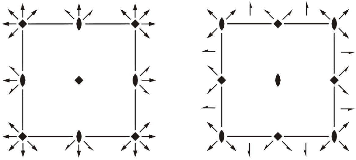
We illustrate the tables of IT A with an example of a diagram of a symmorphic and a nonsymmorphic space group (Figure 3). The diagram on the left-hand side belongs to the space group P422. As in all symbols of space groups, we have as the first item a letter, denoting the centering type of its Bravais lattice. Then follows the symbol of the point group. If this symbol is not modified, the elements of the point group pass through the origin (usually the left top corner of the diagram), and the group is called symmorphic. In the elements of the group P4212 on the right-hand side, we can observe that the two-fold rotations parallel with the plane are moved and, instead of arrows, are ended by half arrows. This means that a shift of half the unit vector is connected with the rotation. Such groups are called nonsymmorphic. Since the symmorphic group has one of the Bravais lattices in combination with all elements of the point group at the origin, the number of symmorphic groups is 73. In nonsymmorphic groups, the symbols of the point group are modified, because the point group operations are associated with certain translations smaller than the cell parameter. Thus, the rotation axes and mirror planes may be combined with certain rational fractions of symmetry translations, leading to screw axes (e.g., 21, 32, 41 or 63) or glide planes (e.g., a, b, c or n). The space groups with the same point group, modified according to these rules, are said to constitute a geometric class of this point group. These geometric classes split further into 73 arithmetic classes in which the groups of a geometric class have the same Bravais lattice. The symbol of an arithmetic class consists of the symbol of the point group followed by the centering symbol of the Bravais lattice (432P, 432I, 432F). The point group of a crystal is called holohedral if it coincides with the point group of the lattice; otherwise, it is called merohedral.
There exist other important groups, which we have recently published with our colleague, Litvin. This was issued in the series of the International Tables of Crystallography, as Vol. E: Subperiodic Groups [12], and contains tables of seven frieze groups, which are one-dimensional groups in two dimensions, 75 rod groups, which have one-dimensional periodicity in three dimensions, and 80 layer groups, which are groups with two-dimensional periodicity in three dimensions. The latter are the most important. They are closely connected with space groups; for each layer group, there exists the space group with the same diagram as the layer group. We have chosen the symbols of these groups as the symbols of the corresponding space group, replacing the lattice letter by lowercase character p or c for a two-dimensional lattice. As a result, we get the nomenclature, which is more like the nomenclature of the Dornberger–Schiff [13] community and different from that used by the International Union. Actually, the groups called plane groups in IT A are two-dimensional groups in two-dimensional space, while layer groups are two-dimensional groups (with a two-dimensional lattice) in three-dimensional space. These tables also contain so-called “scanning tables”, which show how the symmetry of sections of a crystal changes when moving along an axis perpendicular to the section. To each rod group, we can also assign a certain space group, which passes through the origin of the space group. The diagram of the rod group can be identified around the origin of the space group, and the symbol of the rod group is the same as that of the space group with letter P replaced by calligraphic p. These layer and rod groups are actually the factor (quotient) groups of the space group by the partial translation subgroups.
It is of interest that studies of general methods of mathematics, the so-called theory of group extensions [14], applied to space groups by [15], brought new aspects to the theory, which are unfortunately less known and, more unfortunately, ignored, though they will be useful in systematization and in problems of bicrystallography.
We shall now briefly show how the location comes into consideration. Let us assume that we have a space or, generally, a Euclidean group G. According to the fundamental theorem of Euclidean groups [16], every such group can be expressed by a symbol:
Now, we shall see what happens if we move the group by a shift s. We denote the group in a new position by . Systems of non-primitive translations have the property that the sum of two systems is again the system of non-primitive translations, because this also satisfies Frobenius congruences and, hence, defines another space group of the same arithmetic class (G, T). The function φ(g, s) = s − gs, called the “shift function”, is also a system of non-primitive translations, because it satisfies the Frobenius congruences:
Conjugation of by {e|s} leads to the group:
The set of systems of non-primitive translations u(α)(g) + s − gs is therefore an Abelian group , and the set of shifts φ(g, s) is a group . All groups of arithmetic class (G, T) are expressed by , where α distinguishes group types and s the vectors of the fundamental region of the translation normalizer TN(G), which is identical for all groups of the arithmetic class. The relation between a group and implies that we can use Hermann–Mauguin symbols with shift added to specify different position. As an example, we can write or , instead of P4/nbm (origin 2). This notation is used in Vol. E, where we use the symbol or , instead of p4/nbm (origin 2). Vol. E itself proves very well the need to distinguish locations. Thus, the layer group denoted by the symbol indicates that the sectional layer group pnbm appears periodically along the line, perpendicular to the plane (001) at distances (0d) and .
However, it is not even necessary to use the theory of group extensions to show that both of these concepts are unique up to a vector from the fundamental region of the translation normalizer and, hence, may be submitted to a shift in this region. We do not know whether it will have some important consequence. So far, we can point out only one. There have now been International Tables published for years in which we can read subgroups of space groups. All of these tables lose meaning, and the “would be subgroups” must also have proper positions. We can find a lot of examples of wrong subgroups in Vol. A itself. Thus, in the group P42/mnm (No. 136), the group Pn2 (No. 118) is listed as its subgroup. However, the list of symmetry operations of this group contains operations under the numbers 7, 8, 11, 12, which are listed as symmetry operations 3, 4, 7, 8 of the “subgroup”. Neither of these coincides with the operations of the supergroup; to correct it, we have to move the subgroup by .
Crystallographers often argue that abstract groups, like space groups, cannot have a location. However, space groups are groups of operators on a Euclidean space, and as such, they are far from being abstract; they have certainly a location. It is not complicated to improve this situation, but it requires changes in the choices of the origin of groups, and we are afraid that crystallographer would not like this. All of this does not mean that the author wants to diminish in the least the work in Vol. A and recently published Vol. A1 [17]. Both are magnificent and useful books on crystallography, and Vol. A1 contains the shifts of subgroups, unfortunately interpreted as the shift of the origin of a subgroup instead of the subgroup itself.
3. The Magnetic Groups
In 1930, Heesch [18] published an article about groups, which he called the four-dimensional groups of three-dimensional space. Later on (1951), Shubnikov [19] published a book about symmetry and antisymmetry. The story about these groups is long, and there exist many different ideas, interpretations and symbols, mostly of the Russian school. Publications of this period are referred to in IT E [12]. Lifshitz [20] went to great pains to find seven different names for these groups (magnetic groups, Shubnikov groups, Heesch groups, Opechowski–Guccione groups, dichromatic, two-color groups or black and white groups). Finally, the point groups were named and listed by Tavger and Zaitsev [21] as the magnetic point groups. It has been realized that, while the space inversion changes the sign of the ordinary vector, magnetization is a pseudovector, which does not change the sign under space inversion.
Magnetic point groups are necessary if we want to make the right conclusions about macroscopic magnetic properties. For example, if the symmetry is 1′, that of magnetic inversion (called also time inversion), then the object, according to Neuman’s principle cannot be magnetic. There are 32 such groups G ⊗ 1′ (sometimes called gray groups), which bring actually nothing new; they act just as the ordinary 32 classical groups. Opechowski distinguishes the 32 classical point groups—the trivial magnetic groups. The nontrivial magnetic groups are those that contain one half of the classical elements and the other half of the classical elements combined with magnetic inversion g′ = g.e′ (to distinguish the group and the operator, we use letters for the operators: e ≈ 1 for the identity, e′ instead of the inversion group 1′, as well as i ≈ and later .
We follow the derivation of nontrivial magnetic point groups as given by Opechowski [22]. Let us consider a classical group G. It generates a nontrivial magnetic group if we take the halving subgroup F of G and combine elements of its coset (G − F) with magnetic inversion e′. In this way, we obtain the group G(F) = F ∪ e′(G − F). Thus, to derive the 58 (two-colored, black and white) magnetic groups, all we need to do is to find halving subgroups of classical groups. There exist Schoenflies symbols that express the magnetic groups as G(F) with Schoenflies symbols for G and F.
In magnetic crystals, the symmetry is again governed by Neumann’s principle, which we present in slightly different form: the symmetry of the material cannot be higher than the symmetry of the exerted forces. The book containing information about tensors for magnetic point groups is presented by Birss [23] and in a more modern article in IT Vol. D (2003) [24]. The 58 groups are listed below, and in each, we have primed those elements in the symbols that are combined with e′. Thus, we shall consider the group 4z/mz, which has halving subgroups 2z/mz, 4z and z. We take the elements of these subgroups and leave them unchanged, while the elements of the coset to the subgroups are combined with magnetic inversion e′. As a result, we obtain the magnetic groups , and or, in Schoenflies notation, C4h(C2h), C4h(C4) and C4h(S4). It may help very much if we consider the action of the reflections on magnetization. If we reflect an ordinary vector in a plane parallel to it, it does not change, but reflected in a normal plane, it changes its sign. The magnetic vector, if parallel with a plane, changes its sign, but keeps it when perpendicular to the plane. This is so because reflection in a plane equals inversion times two-fold rotation about an axis perpendicular to this plane.
Applying the described procedure to the 32 ordinary groups, we get the 58 groups listed below, which are distributed in seven crystal systems, such that each group belongs to the same system as the group without primes. Let us not forget that now, the groups with classical symbols may allow magnetism, like the group 2z/mz allows magnetism along the 2z axis. Thus, the total number of groups that we obtain is 122 = 32 + 32 + 58. We should, however, remember that only 90 of them are so far candidates for magnetism, while 32 groups with a primed unit are automatically eliminated. The symbols in the table are the Hermann–Mauguin symbols.
The 58 magnetic point groups, triclinic, monoclinic and orthorhombic, are in the first row, then tetragonal, trigonal, hexagonal and cubic.
Another big contribution to the magnetic groups has been achieved in derivation of magnetic space groups. Their list was originally reported by Zamorzaev [25], later by Belov et al. [26] and, then, by Opechowski and Guccione [27]. Then, Koptsik [28] published a book with diagrams of black and white space groups under the name Shubnikov groups. This book is now so rare that it is hardly available. However, our friend, D.B. Litvin from Penn State University, decided that it would be fine if we had diagrams of magnetic space groups in the style of Vol. A and other magnetic groups, including the magnetic frieze, rod and layer groups. Derivation and nomenclature is the same as for the point groups. In particular, the nontrivial space groups are derived with the use of halving subgroups. Notice, that the halving subgroup can be due either to halving of the point group or to halving of the Bravais lattice. These groups are divided into 230 superfamilies according to the classical groups from which they are derived and 80 layer superfamilies, 75 rod and seven frieze superfamilies. The total number of magnetic space group types is 1651, of layer groups 580, of rod groups 399 and of frieze groups 31. There are 36, 11, 2 and 2 magnetic Bravais lattices, respectively. Accordingly, he produced the diagrams of all of these groups, as well as the diagrams and numerical data of atomic positions and magnetic moment orientation. One example of such a diagram and a diagram of atomic positions are given in the next figure. This is from an electronic book available on the Internet [29].
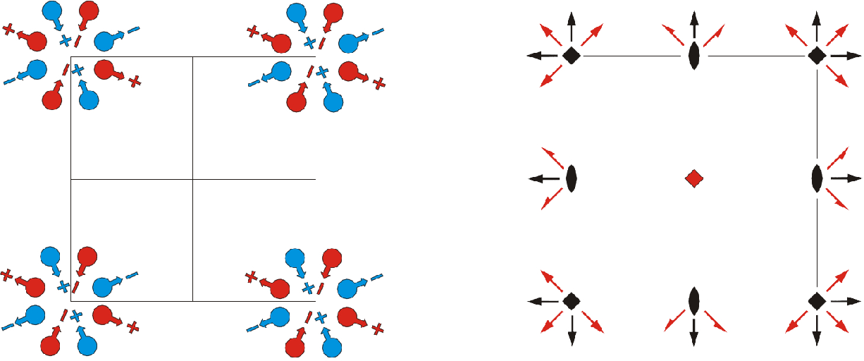
These magnetic groups have some properties common with the classical space groups (Figure 4). There exist 11 pairs of chiral superfamilies and 73 symmorphic superfamilies, and to each of the groups of the 580 superfamilies of the layer groups, there are corresponding superfamilies of space groups, which have the same diagrams as the layer groups; and the analogous relation exists for rod groups. This is a consequence of the fact that the superfamily of the decomposable or reducible space group contains decomposable or reducible groups. Furthermore, the magnetic groups should be shifted in space in the whole of the superfamilies.
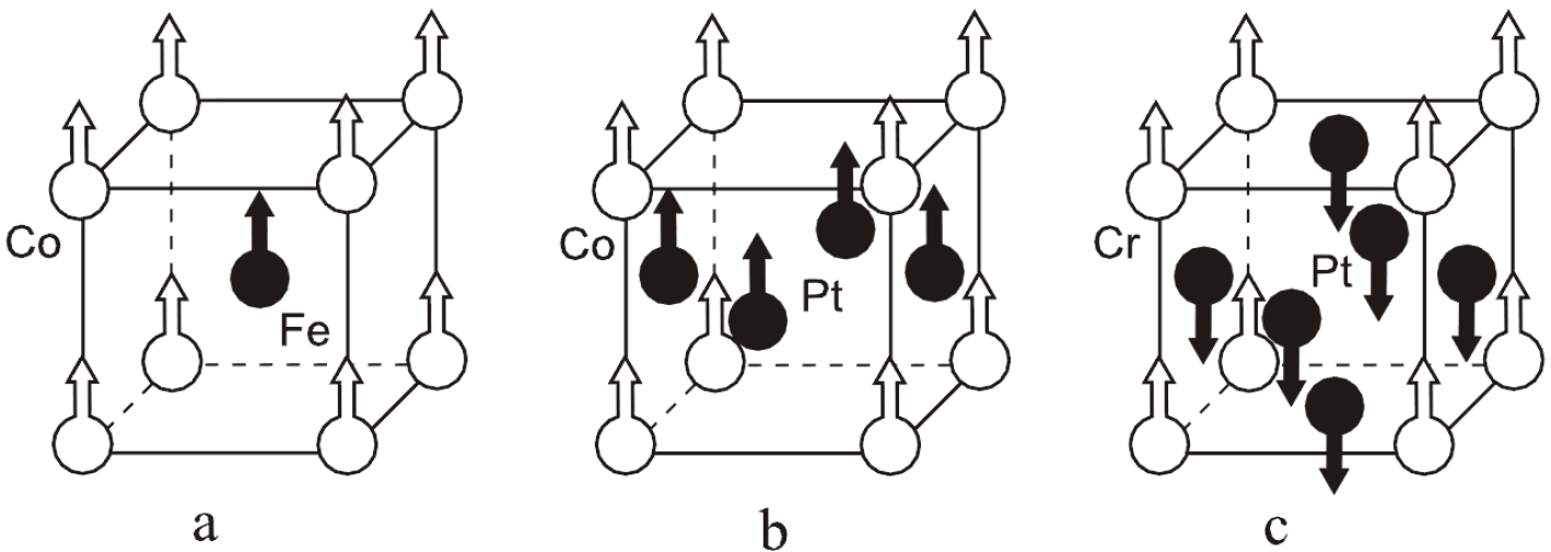
The relationship between magnetic structures and their magnetic groups were studied, for example, in [30], from which we illustrate a few examples. Some other examples are courtesy of D.B. Litvin. Figure 5a–c shows the structures of α′-FeCo, CoPt and CrPt3 as they appear at phase transitions below temperatures of 1390 K, 813 K and 530 K from structures of symmetries of Pmm, P4/mmm and Pmm (Figure 5). The first two structures are ferromagnetic; the third is ferrimagnetic; the magnetic symmetries of all three are P4/mm′m′. An alloy MnFe2 has the magnetic symmetry . The Heusler alloy Cu2MnAl has a paramagnetic structure Fmm, which transforms below 603 K into a ferromagnetic structure of symmetry Rm′, and CsCoCl3, where only Co is magnetic, acquires a canted ferrimagnetic structure of symmetry P2bcca (Figure 6). All compounds, with the exception of the last one, have a classical Bravais lattice, while the last one has the magnetic lattice P2b. It should be also noted that the transitions to magnetic cases are phase transitions and, hence, result in domain structures. For example, in the first and third case (Figure 5a,c), these are the transition to a phase with six domains, and the second (Figure 5b) leads to two domains. The magnetic groups are related to one of the domains.
4. Magnetoelectricity
Various phenomena were studied in which the magnet was submitted to external mechanical forces, e.g., the piezomagnetic effect, where an external mechanical force induces magnetism. However, in more recent times, interest has focused on the interaction of electric and magnetic fields. The magnetoelectric effect is a phenomenon of inducing magnetization by an electric field or vice versa. This effect may be observed in single or composite cases (Cr2O3). In multiferroic materials, we observe a coupling between the magnetic and electric order parameters. Composite magnetoelectrics are combinations of magnetostrictive and electrostrictive materials, such as ferromagnetic and piezoelectric materials. The size of the effect depends on the microscopic mechanism.
In 1973, there was a conference on the magnetoelectric effect in Seattle. The phenomena of magnetoelectricity is of interest itself and is characterized by coefficients αij, βijk and γijk, corresponding to the contribution to the thermodynamic potential, where P is the electric polarization, M the magnetization, E and H the external electric and magnetic field and α, β and γ the linear and nonlinear ME susceptibilities. Some examples of single-phase magnetoelectrics have been demonstrated at this conference. In single-phase magnetoelectrics, the effect can be due to the couplings of magnetic and electric orders, as observed in some multiferroics. In composite materials, the effect originates from interface coupling effects, involving strain. Some of the promising applications of the ME effect are the sensitive detection of magnetic fields, advanced logic devices and tunable microwave filters.
At that conference, Schmid [31] expanded the thermodynamic potential ginto a Taylor series in E and H:
The magnetoelectric effect of first order has been considered by O’Dell [32], who presented forms of the first order magnetoelectric tensor αik for all magnetic groups. Schmid showed that out of the 58 magnetic point groups allowing the linear magnetoelectric effect, there are 19 groups that do not allow the nonlinear effects EHH and HEE. Twenty one point groups allow only the magnetoelectric effect of the type HEE. At the conference, Schmid [31] calculated all magnetic point groups that allow the terms EHH and HEE, whereas Ascher [33] considered kineto-magnetic and kineto-electric effects in moving crystals.
The relations between inversions and fields are shown in the following Table 1. The operators of inversion either change the sign of the field or leave it invariant. Normally, we expect the existence of the electric and magnetic field. However, from the group theoretical relations in the character table, we see that the existence of another field, which we name toroidic (this is how Ascher’s kinetic effects of electric currents are now interpreted), should be expected. The unit element and inversions are again denoted by letters instead of the symbols of groups. The parities defined by letters are later given in a representation table.
Ascher left some unpublished notes, which were later picked up and discussed by Schmid and Janovec, who also did not publish his results. I am now taking the liberty to publish some results with his kind permission. The toroid itself is well known from electrical engineering. It consists of a kernel of the form of an anuloidon which there is a wire coiled in the same direction, so that the magnetic field from the current has the form of a circle and intensity . Accordingly, there is a toroidal moment T created, perpendicular to the plane of the magnetic field. There remains only the question of the conjugate variable to this moment. It is possible and quite sound to consider as such the electric current j, so that the contribution to a potential equals jdT.
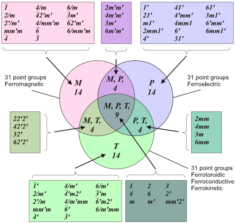
Among Ascher’s notes, there was a diagram later published by Schmid [34], who called it trinity (Figure 7). It contains three intersecting circles, in which the groups are written, which allow ferromagnetism, ferroelectricity and ferrotoroidic fields. In the section of these, we obtain 14 groups, which allow only polarization, 14 groups, which allow magnetization, and 14 groups, which allow toroidal moment. Checking the groups that meet at the intersection of the two circles, we meet in each case four groups, which allow a pair of these properties, i.e., three regions in which two of the properties may occur. Taking the middle of the diagram, where all three circles intersect, we obtain the region and nine groups, which allow all three phenomena. Thus, there are 31 groups allowing each of the phenomena.
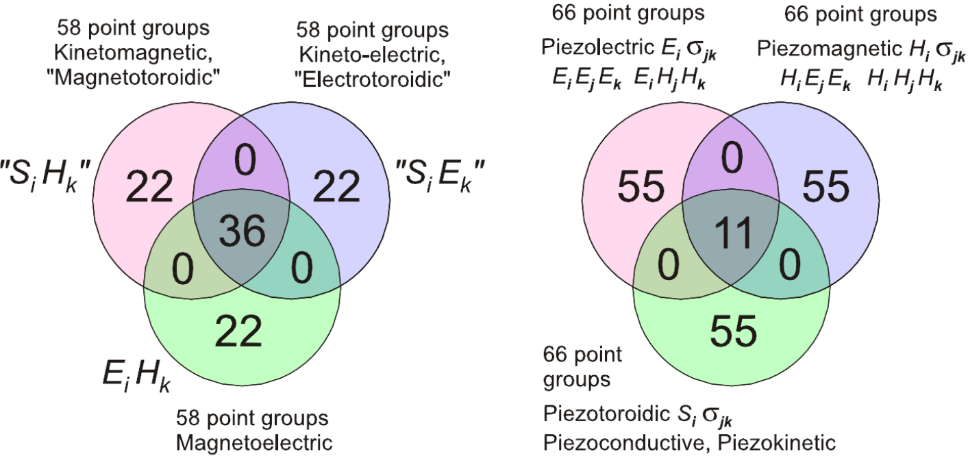
Schmid [34] added to it two diagrams (Figure 8), in which groups allowing higher order tensors and their numbers are given. It is clear from Schmid that the formulas given on page 136 only show the first terms of a Tailor series.
There remain two problems. First, the current j here should be interpreted as reversible current, while in reality, the current as a thermodynamic quantity is not reversible. We can interpret it as a superconductive current. The toroidic moment is interpreted in known experiments as a result of a quantum mechanical phenomenon, microscopic currents, and hence, in principle, it is reversible. Another problem is the interpretation of the magnetic field switching. This should also be reversible. It seems that a rather elegant solution is proposed by Janovec [35]. We should distinguish two varieties of time: the reversible and the irreversible. This actually corresponds to reality. The reversible time concerns the microscopic processes, i.e., all of the processes (equations), described by reversible equations, that do not change if we change the sign of the time. The actual processes are happening in real time, which is irreversible (previously, we called this inversion the magnetic inversion, but instead, we can talk about thermodynamic time and its inversion).
A comment concerning the application of inversions: The concept of inversions is rather elusive, and we should think about their meaning. Such inversions can be applied only in a limited region in a finite time, and we can attempt to realize them by the switching of electric, magnetic or toroidic field. An inversion cannot be certainly applied to the whole universe or at an instant of time. Indeed, we cannot switch space upside down, neither can we do it with some rigid body, nor can we switch the direction of time. If we apply space inversion in the form of field reversal, it will certainly not turn the objects upside down, but if we change the direction of an electric field from one direction of the z-axis to the opposite, it will change the chirality of the whole space, and we shall observe left-handed objects as right-handed and vice versa. If we take the magnets, described in the first part, and switch the applied magnetic field, we can expect the reversal of currents and of magnetization in diamagnets, but in para- and ferro-magnets, we expect demagnetization depending on the strength of the reversed field; additionally, this will take a finite time.
Hence, Janovec proposes introducing two types of time, microscopic time, which is reversible (in view of a rough model, however simplified, of the Big Bang, we have to believe that even this microscopic time cannot be reversible in long time intervals), and macroscopic or thermodynamic time, which corresponds to real processes in which everything tends to disorder. However, this time cannot be reversible. Hence, the process assumes that this time can achieve only two variables, plus and minus. The real process runs either forwards or backwards. If we reverse the direction of time, the processes simply run as if in opposite direction, which, however, cannot be distinguished from the original. In the literature, we meet different names: There is the “time inversion” as the most frequently used term, which, however, may apply only to microscopic processes. We have used the term “magnetic inversion” to distinguish it from microscopic time inversion, but now, we believe that it is necessary to distinguish between “time inversion” for microscopic time and for the thermodynamic time. However, Janovec’s idea of two-valued time seems to us not acceptable.
Another result from this congress is connected with the name of Opechowski. He observed that the numbers of groups that allow certain phenomena coincide with the numbers of other groups that allow other phenomena, and he called them the magic numbers [36]. The author of this study explained the existence of these numbers by showing that, if the tensor of a certain property has a certain form, certain components of which are invariant, then there exists another property, which has the same form under the action of another group [37]. An analogous conclusion has been reached by Grimmer [38], and finally, the author proved a general principle of relations between groups and tensor properties under the name of Opechowski’s magic relations [39].
Opechowski’s magic numbers are clear at once from the trinity diagrams. From the first diagram, we see that the number of groups allowing ferroelectricity is 31, the same as the numbers of groups allowing ferromagnetism or ferrotoroidicity. From the other two diagrams, we can see that the number of groups that allow magnetoelectricity, magnetotoroidic or electrotoroidic effects is 58, and the number of groups allowing piezoelectricity, piezomagnetism and piezotoroidicityis 66.
To understand the theorem on Opechowski’s magic relations, we should know at least a little bit about the so-called representation theory of groups. We shall consider representation theory using tables for the oriented group D4z and its operator isomorphs, acting on tensors of intrinsic symmetry of the piezoelectric tensor, as an example. Though the theory is exceedingly simple, very few people know it. It is based on so-called Clebsch–Gordan products. These two names and the respective mathematical procedure have been well known for a long time to atomic physicists, where Clebsch–Gordan coefficients are widely tabulated for the group O(3). It has been shown that Clebsch–Gordan coefficients have meaning also for crystallographic point groups [40]. The last procedure is to transcribe these coefficients in the form of Clebsch–Gordan products, which are more suitable for further calculations [41].
Notice that 11 tables of Clebsch–Gordan products for groups of proper rotations are sufficient.
The simplicity of the method is rather well illustrated by a paper on gyrotropic phase transitions [42].
The first table (Table 2) you see below defines representations of the group D4z in a specific orientation. The remaining three groups are operator isomorphic groups of the same oriented Laue class, so that they transform the variables in the same manner under the respective generators. Now, the principle of the calculation uses the fact that no group of this type may act on some variables that do not transform according to this table. This property is called reducibility, and we have met it in the first half. You may have the group of this type acting on a thousand variables, but these can be divided into four single variables and a pair, which either change the sign or transform as the pair (x1, y1), which transform by the matrix D(1)(2z)(x1, y1) = 2z(x1, y1) = (y1, −x1), and there can be a lot of these pairs as, for example, in the decomposition of piezoelectric tensor.
Hence, the first table is the table of representations. Such tables are known for all point groups together with other useful information by [43]. The second table (Table 3) may be called the Clebsch–Gordan table. As you can see, the first line contains all four one-dimensional and one two-dimensional variables. Under each variable, the bilinear combination of those variables is written, which transforms like the variable above. However, it is easy to find the meaning of vector components, for the groups D4z: (x1, y1) are exactly the components of an ordinary vector, while z transforms like the variable x2. Thus, using the Clebsch–Gordan table, we see that x2(x, y) transforms like (−zy, zx), i.e., like components of second rank tensor (−u32, u31). This way, we can consecutively calculate the decomposition of higher rank tensors [41]. Using in addition Opechowski’s magic relations, we can relatively easily find the decomposition of rather high rank tensors.
Let us recall that a tensor decomposition means an expression of combinations of its coordinates into quantities that transform according to group representations (see the table of tensorial decompositions of the piezoelectric tensor below). It is simply a transformation of tensor coordinates to another coordinate system in the space of tensors, so that the number of combinations is equal to the number of original tensor components. To find the allowed form of a tensor, we have to put to zero all components that transform by other rules than the invariants x1. The knowledge of invariants is what we look for as allowed properties, and the other components are useful in the phase transition theory.
To describe these relations at least in one case, we present below a table that we call Opechowski’s Tableaux (Table 4). It contains 16 operator groups isomorphic with the group of proper rotation 4z2x2xy. We know two basic facts: (1): all tensors of the same intrinsic symmetry (of four possible parities) transform by the same way under the group of proper rotations; and (2) the tensor of positive parity with respect to all inversions transforms in the same way under all groups of the oriented Laue class. Of these groups, three have the same structure with reference to the inversions, like the first group multiplied in a sequence by x1, x2, x3 and x4. In the last three columns, we give one of these variables on the intersection with the row of a group and a column of one of the three inversions, which are denoted by scalars of electric, magnetic and toroidal types ε, τ and ετ. However, the rows in the table of tensors are labeled in the same sequence. Hence, if we want now the decomposition of a piezomagnetic tensor for a group for which we got the variable x4 in a table, we obtain its tensor decomposition in the fourth row, because the piezomagnetic tensor differs by multiple x4 from the piezoelectric tensorin the table. Here, it sounds too complicated, but in fact, it is rather easy. We obtain also one conclusion: For the three groups that have four one-dimensional representations, we obtain four types of possible decompositions. Analogously, we obtain four different decompositions for the Laue class 2x2y2z(D2z) and 6z2x2y (D6z). Generally, the number of different decompositions for groups of a given Laue class equals the number of one-dimensional representations of these groups. Thus, we have two decompositions for groups with two one-dimensional irreducible representations (2z (C2z), 3z2x (D3z), 4z (C4z), 6z (C6z) and 432 (O)) and only one decomposition for the groups with one one-dimensional irreducible representation (1 (C1), 3z (C3z) and 43 (T)). Hence, there exist only 23 possible tensor decompositions for the four tensors of different parities, but the same intrinsic symmetry. Each of them implies one allowed tensor component.
Since we know the decompositions of some tensors up to the fourth rank, we may give a fair promise that all decompositions will be soon published. Notice that the decomposition contains more information than just the knowledge of the invariant tensor. It contains as many components as the original tensor, but in different combinations, and it is a good background for consideration of phase transitions.
We would like to emphasize the last mentioned property of Clebsch–Gordan products. We have, as already said, to consider these products only for 11 groups of proper rotations. Each of these groups has a certain number of isomorphic (more exactly, operator isomorphic) groups among magnetic point groups, but we can use the Clebsch–Gordan products for all of them. The meaning of one-dimensional variables shall be different for the basic vectors (pseudovector, electrical, magnetic and toroidal moment), so that the derived tensors will be different for the isomorphic groups. Furthermore, the tensor multiplication will provide not only the invariant tensors, but the full decomposition, which may itself be used in consideration of structural phase transitions [44]. The number of different decompositions is equal to the number of one-dimensional representations of the group of proper rotations. For groups with four, such representations have only four types of decompositions, and hence, each of them appears twice.
5. Conclusions
This article is considered an essay, and hence, we allowed ourselves some discussions and personality. We discussed the question about group location, which is connected with the question about the uniqueness of Hermann–Mauguin symbols and of the origin choice. Practicing crystallographers argue that Euclidean groups as abstract groups cannot have any location. However, Euclidean and magnetic groups are groups of operators and, hence, far from being abstract. They are geometrical objects, and as such, they certainly have a location, though the range of their positions is only a fraction of the unit cell. We gave elementary proof of this assertion. In our opinion, this analysis should be reflected in IT A, and it is done in Vol. A1. As a practical consequence, we can consider equitranslational domains in phase transitions, domain walls and twin boundaries.
Another problem is of terminological character. We find that the name magnetic groups is actually wrong in the sense that it does not represent the reality. Actually, all point groups that are multiple with the element of the time inversion 1′ are nonmagnetic, and this is the proper notation for the ordinary nonmagnetic materials. Each ordinary group G is directly multiplied by time inversion, so that it is denoted G′. On the other hand, most of the ordinary 32 symmetries describe frequently magnetic materials, as well as some of the remaining 58 symmetries.
Finally, about the terminological problem. Opechowski used to call the three-dimensional space with time as the fourth coordinate of Newton’s space. It would be then natural to call the magnetic groups as Newton’s groups, so that we shall have point, frieze, rod, layer and three-dimensional (or space) Newton groups in parallel with Euclidean point, frieze, rod, layer and space groups. However, the Lifshitz count [20] of various names convinced me to let the name magnetic groups stand and coin it as standard. This is a decision to be made by the International Union of Crystallography.
Acknowledgments
I would like to thank D. B. Litvin and V. Janovec for valuable discussions, as well as to my son, Vojtěch, for patience with drawing the figures. Greatest thanks are due to one of the referees for his invaluable help with my insufficient English.
Conflicts of Interest
The author declares no conflict of interest.
References
- Nye, J.F. Physical Properties of Crystals; Clarendon Press: Oxford, UK, 1957; Revised edition; Oxford University Press: Oxford, UK, 1985.
- Sirotin, Y.I.; Shaskolskaya, M.P. Fundamentals of Crystal Physics; Nauka: Moscow, Russia, 1979; Translated by Mir: Moscow, Russia; 1982.
- Hessel, J.F.C. Kristal. In Gehler’s Physikalisches Wörterbuch; Schwickert: Leipzig, Germany, 1830; Volume 5, pp. 1023–1360. [Google Scholar]
- Gadolin, A.V. Deduction of all crystallographic systems and their subdivision by means of a single general principle. Ann. Imp. St. Petersburg Mineral Soc. 1867, 112–200, in Russian. [Google Scholar]
- Sohncke, L. Entwicklung Einer Theorie der Kristallstruktur; Teubner: Leipzig, Germany, 1879. [Google Scholar]
- Schwarzenberger, R.L.E. N-Dimensional Crystallography; Pitman: San Francisco, CA, USA, 1980. [Google Scholar]
- Brown, H.; Bülow, R.; Neübüser, J.; Wondratschek, H.; Zassenhaus, H. Crystallographic Groups of Four-Dimensional Space; Wiley and Sons: Toronto, ON, Canada, 1978. [Google Scholar]
- Janssen, T.; Janner, A.; Looijenga-Vos, A.; de Wolff, P.M. Incommensurate and Commensurate Modulated Structures. In International Tables for Crystallography, Vol. C, Mathematical, Physical and Chemical Tables; Prince, E., Ed.; Kluwer Academic Publishers: Dordrecht, The Netherlands, 2006; pp. 906–955. [Google Scholar]
- Niggli, P. Geometrische Kristallographie des Diskontinuums; Borntraeger: Leipzig, Germany, 1919; in German. [Google Scholar]
- Hermann, C. Internationale Tabellen zur Bestimmung von Kristallstrukturen, 1. Band; Borntraeger: Berlin, Germany, 1935. [Google Scholar]
- Hahn, T. International Tables for Crystallography. Vol. A: Space Group Symmetry; IUCr and Kluver: Dordrecht, The Netherlands, 1983. [Google Scholar]
- Kopský, V.; Litvin, D.B. International Tables for Crystallography. Vol. E: Subperiodic Groups; IUCr and Kluwer: Dordrecht, The Netherlands, 2002. [Google Scholar]
- Grell, H.; Krause, C.; Grell, J. Tables of the 80 Plane Space Groups in Three Dimensions; Akademie der Wissenschafteen der DDR: Berlin, Germany, 1989. [Google Scholar]
- Ascher, E.; Janner, A. Algebraic aspects of crystallography. I. space groups as extensions. Helv. Phys. Acta. 1965, 38, 551–572. [Google Scholar]
- Ascher, E.; Janner, A. Algebraic aspects of crystallography. II. Non-primitive translations in space groups. Commun. Math. Phys. 1968/69, 11, 138–167. [Google Scholar]
- Kopský, V. Is a revision of Vol. A of the International Tables for Crystallography Desirable or Necessary? In Advances in Structure Analysis; Kužel, R., Hašek., J., Eds.; Czech and Slovak Crystallographic Association: Prague, Czech Republic, 2001. [Google Scholar]
- Wondratschek, H.; Müller, U. International Tables of Crystallography. Vol. A1: Symmetry Relations between Space Groups; Kluwer: Dordrecht, The Netherlands, 2004. [Google Scholar]
- Heesch, H. Ueber die vierdimensionalen Gruppen des dreidimensionalen Raumes. Z. Kristallogr. 1930, 73, 325–345. [Google Scholar]
- Shubnikov, A.V. Symmetry and Antisymmetry of Finite Figures; Nauk, A., Ed.; USSR: Moscow, Russia, 1951; in Russian. [Google Scholar]
- Lifshitz, R. Magnetic Point Groups and Space Groups; Tel Aviv University: Tel Aviv, Israel, 2004. [Google Scholar]
- Tavger, B.A.; Zaitsev, V.M. Magnetic Symmetry of Crystals. Zh. Exp. Teor. Fiz. 1956, 30, 564–568, in Russian. [Google Scholar]
- Opechowski, W. Crystallographic and Metacrystallographic Groups; North Holland: Amsterdam, The Netherlands, 1986. [Google Scholar]
- Birss, R.R. Symmetry and Magnetism; North Holland: Amsterdam, The Netherlands, 1964. [Google Scholar]
- Borovik-Romanov, A.S.; Grimmer, H. Magnetic Properties. In International Tables for Crystallography, Vol. D, Physical Properties of Crystals; Authier, A., Ed.; Kluwer Academic Publishers: Dordrecht, The Netherlands, 2003; pp. 105–149. [Google Scholar]
- Zamorzaev, A.M. Generalization of the Fedorov Groups. Ph.D. Dissertation, Leningrad State University, Leningrad, Russia, 1953; in Russian. [Google Scholar]
- Belov, N.V.; Neronova, N.N.; Smirnova, T.S. Shubnikov groups. Kristallografiya 1957, 2, 315–325, in Russian. [Google Scholar]
- Rado, G.T.; Suhl, H. Magnetic Symmetry. In Magnetism; Rado, G.T.; Suhl, H. Academic Press: New York, NY, USA, 1965; pp. 105–165. [Google Scholar]
- Koptsik, A.V. Shubnikov Grups; Moscow University: Moscow, Russia, 1966; in Russian. [Google Scholar]
- Litvin, D.B. Magnetic Group Tables: 1-, 2-, and 3-Dimensional Magnetic Subperiodic Groups and Magnetic Space Groups, Available online: http://www.iucr.org/publ/978-0-9553602-2-0 accessed on 6 January 2015.
- Laughlin, D.E.; Willard, M.A.; McHenry, M.E. Magnetic Ordering: Some Structural Aspects. In Phase Transitions and Evolution of Materials; Turchi, P., Gonis, A., Eds.; The Minerals, Metals and Material Society: Warrendale, PA, USA, 2000; pp. 121–137. [Google Scholar]
- Schmid, H. On a magnetoelectric classification of materials. Int. J. Magn. 1973, 4, 337–361. [Google Scholar]
- O’Dell, T.H. The Electrodynamics of Magneto-Electric Media; North Holland: Amsterdam, The Netherlands, 1970. [Google Scholar]
- Ascher, E. Kinetoelectric and Kinetomagnetic Effects in Crystals. Int. J. Magn. 1979, 5, 287–295. [Google Scholar]
- Schmid, H. Some symmetry aspects of ferroics and single phase multiferroics. J. Phys. 2008, 434231:1–434231:24. [Google Scholar]
- Janovec, V. Personal communication, May 2013.
- Opechowski, W. Magneto electric Symmetry. Int. J. Magn. 1974, 5, 317–325. [Google Scholar]
- Kopský, V. The structure of Heesch groups and its relation to material property tensors. J. Magn. Magn. Mat. 1976, 3, 201–211. [Google Scholar]
- Grimmer, H. General connections for the form of property tensors in the 122 Shubnikov point groups. Acta Cryst. A 1991, 47, 226–232. [Google Scholar]
- Kopský, V. Opechowski’s magic relations. Zs. Kristallogr. 2006, 221, 51–62. [Google Scholar]
- Koster, G.F.; Dimmock, J.O.; Wheeler, R.G.; Statz, H. Properties of the Thirty-Two Point Groups; MIT Press: Cambridge, MA, USA, 1963. [Google Scholar]
- Kopský, V. The use of the Clebsch-Gordan reduction of the Kronecker square of the typical representation in symmetry problems of crystal physics. Part I. and II. J. Phys.C Solid St. Phys. 1976, 9, 3405–3420. [Google Scholar]
- Koňák, C.; Kopský, V.; Smutný, F. Gyrotropic phase transitions. J. Phys. C Solid St. Phys. 1978, 11, 2493–2518. [Google Scholar]
- Altmann, S.L.; Herzig, P. Point-Group Theory Tables; Clarendon Press: Oxford, UK, 1994. [Google Scholar]
- Kopský, V. Tensor Parameters of Ferroic Phase Transitions. I: Theory and Tables. Phase Trans. 2001, 73, 1–422. [Google Scholar]


| Field | e | i | e′ | i′ | Property | Parity |
|---|---|---|---|---|---|---|
| State without fields | 1 | 1 | 1 | 1 | charge density ρ | x1 |
| Electric field E | 1 | −1 | 1 | −1 | polarization Px, Py, Pz | x2 |
| Magnetic field H | 1 | 1 | −1 | −1 | magnetization Mx, My, Mz | x3 |
| Toroidic field K | 1 | −1 | −1 | 1 | spontaneous current jx, jy, jz | x4 |
| D4z − 4z2x2xy | 4z | 2x |
|---|---|---|
| C4vz − 4zmxmxy | 4z | mx |
| D2dz − z2xmxy | z | 2x |
| D4z = zmx2xy | z | mx |
| χ1(x1) | 1 | 1 |
| χ2(x2) | 1 | −1 |
| χ3(x3) | −1 | −1 |
| χ4(x4) | −1 | −1 |
| D(1)(x1, y1) |
| x1 | x2 | x3 | x4 | (x1, y1) |
|---|---|---|---|---|
| x3x4 | x2x4 | x2x3 | x2(y1, −x1) | |
| x1y1 − y1x1 | x1y1 + y1x1 | x3(x1, −y1) | ||
| x4(y1, x1) |
| Ireps with associated inversions | Transformation of nontrivial properties scalars | ||||||
|---|---|---|---|---|---|---|---|
| Class | Group | i | e′ | i′ | ε | τ | ετ |
| D4 | 4z2x2xy | χ1 | χ1 | χ1 | x1 | x1 | x1 |
| D4(C4) | χ1 | χ2 | χ2 | x1 | x2 | x2 | |
| D4(D2) | χ1 | χ3 | χ3 | x1 | x3 | x3 | |
| χ1 | χ4 | χ4 | x1 | x4 | x4 | ||
| C4v | 4zmxmxy | χ2 | χ1 | χ2 | x2 | x1 | x2 |
| C4v(C4) | χ2 | χ2 | χ1 | x2 | x2 | x1 | |
| C4v(C2v) | χ2 | χ3 | χ4 | x2 | x3 | x4 | |
| χ2 | χ4 | χ3 | x2 | x4 | x3 | ||
| D2d | z2xmxy | χ3 | χ1 | χ3 | x3 | x1 | x3 |
| D2d(S4) | χ3 | χ2 | χ4 | x3 | x2 | x4 | |
| D2d(D2) | χ3 | χ3 | χ1 | x3 | x3 | x1 | |
| χ3 | χ4 | χ2 | x3 | x4 | x2 | ||
| zmx2xy | χ4 | χ1 | χ4 | x4 | x1 | x4 | |
| χ4 | χ2 | χ3 | x4 | x2 | x3 | ||
| χ4 | χ3 | χ2 | x4 | x3 | x2 | ||
| χ4 | χ4 | χ1 | x4 | x4 | x1 | ||
| D4z – 4z2x2xy | d31 + d32 | d36 | d31 – d32 | (d11, d22) | (d12, d21) | x1 | |
| d33 | (d13, d23) | (d26, d16) | |||||
| d14 – d25 | d15 + d24 | d14 + d25 | d15 – d24 | (d35, d34) | |||
| C4vz – 4zmxmxy | d31 + d32 | d31 – d32 | d36 | (d22, −d11) | (d21, −d12) | x2 | |
| d33 | (d23, −d13) | (d16, −d26) | |||||
| d15 + d24 | d14 – d25 | d15 – d24 | d14 + d25 | (d34, −d35) | |||
| D2dz – z2xmxy | d36 | d31 – d32 | d31 + d32 | (d11, −d22) | (d12, −d21) | x3 | |
| d33 | (d13, −d23) | ||||||
| d14 + d25 | d15 – d24 | d14 – d25 | d15 + d24 | (d35, −d34) | (d26, −d16) | ||
| d31 – d32 | d36 | d31 + d32 | (d22, d11) | (d21, d12) | x4 | ||
| d33 | (d23, d13) | ||||||
| d15 – d24 | d14 + d25 | d15 + d24 | d14 – d25 | (d34, d35) | (d16, d26) | ||
© 2015 by the authors; licensee MDPI, Basel, Switzerland This article is an open access article distributed under the terms and conditions of the Creative Commons Attribution license (http://creativecommons.org/licenses/by/4.0/).
Share and Cite
Kopský, V. Crystallography and Magnetic Phenomena. Symmetry 2015, 7, 125-145. https://doi.org/10.3390/sym7010125
Kopský V. Crystallography and Magnetic Phenomena. Symmetry. 2015; 7(1):125-145. https://doi.org/10.3390/sym7010125
Chicago/Turabian StyleKopský, Vojtěch. 2015. "Crystallography and Magnetic Phenomena" Symmetry 7, no. 1: 125-145. https://doi.org/10.3390/sym7010125