Symmetry-Breaking as a Paradigm to Design Highly-Sensitive Sensor Systems

Abstract

A large class of dynamic sensors have nonlinear input-output characteristics, often corresponding to a bistable potential energy function that controls the evolution of the sensor dynamics. These sensors include magnetic field sensors, e.g., the simple fluxgate magnetometer and the superconducting quantum interference device (SQUID), ferroelectric sensors and mechanical sensors, e.g., acoustic transducers, made with piezoelectric materials. Recently, the possibilities offered by new technologies and materials in realizing miniaturized devices with improved performance have led to renewed interest in a new generation of inexpensive, compact and low-power fluxgate magnetometers and electric-field sensors. In this article, we review the analysis of an alternative approach: a symmetry-based design for highly-sensitive sensor systems. The design incorporates a network architecture that produces collective oscillations induced by the coupling topology, i.e., which sensors are coupled to each other. Under certain symmetry groups, the oscillations in the network emerge via an infinite-period bifurcation, so that at birth, they exhibit a very large period of oscillation. This characteristic renders the oscillatory wave highly sensitive to symmetry-breaking effects, thus leading to a new detection mechanism. Model equations and bifurcation analysis are discussed in great detail. Results from experimental works on networks of fluxgate magnetometers are also included.

1. Introduction

Symmetry in nonlinear dynamical systems can force certain regions of their phase-space to be invariant under the governing equations. That is, any solution trajectory that starts in one of those regions remains there forever. Furthermore, it is well-known that the presence of invariant regions in continuous dynamical systems can lead to cyclic trajectories that connect, through these invariant subspaces, steady states, periodic oscillations and even chaotic sets [1,2]. These cycles, which are also known as heteroclinic cycles, are robust under perturbations that preserve the symmetry of the system. Over the past twelve years, we have developed an innovative concept for developing highly-sensitive sensor technologies based on a network architecture of oscillators and the robustness of heteroclinic cycles. The fundamental principle is to exploit the architecture of the network to generate coupling-induced stable periodic oscillations, thus minimizing power requirements to operate the sensors. The oscillations emerge through a global branch of heteroclinic connections between steady states, so that near the onset of the cycle, the accompanying oscillations exhibit long periods, which in turn renders their waveform highly sensitive to symmetry-breaking effects caused by very small external signals. This critical observation has led to the fabrication of highly-sensitive sensors, magnetic- and electric-field ones, whose operation relies mainly on the coupling signal that travels from one bistable system to the next one [3–6]. That is, in the absence of coupling, each bistable unit cannot oscillate. In practice, the bistable units are not exactly identical. Experimental measurements show that system parameters vary within a range of ±5%, so the network system is not perfectly symmetric. However, computational works show that remnants of the cycle persist under ±10% variations in system parameters. There are many engineering designs of sensor systems that seek to advance sensitivity levels through smart materials, whose properties can be significantly altered in a controlled fashion by external stimuli, such as stress, temperature or moisture. However, the symmetry-based design described in this review is the only sensor system that incorporates in a systematic way advanced ideas and concepts from nonlinear dynamics, such as heteroclinic connections, global bifurcations, computational group theory and network topologies.

In this review article, we provide a self-contained description of the basic ideas and results of the modeling and analysis of this new paradigm. The description is aimed mainly at networks of fluxgate magnetometers coupled via magnetic flux. The network architecture is a ring with a preferred orientation, i.e., unidirectionally coupling, which leads to a ring array with Z_N-symmetry, where Z_N is the group of cyclic permutations of N objects. In addition, we also review another prototypical network system made up of coupled overdamped Duffing elements, which describe the dynamics of the polarization inside a ferroelectric material. This latter network system is the basis of an electric field sensor, currently under development. In both cases, magnetic and electric field sensors, our analysis shows that if N is odd, then unidirectionally-coupled elements with cyclic boundary conditions would oscillate when a control parameter, i.e., coupling strength, exceeds a critical value. However, the oscillatory behavior can also be seen for large even values of N, because as N increases, the basins of attraction for equilibrium and oscillations become rather small, and numerical errors can easily induce the system to switch from one basin to another, similar to a real physical system influenced by noise. Typically, the oscillations emerge with an infinite-period through a heteroclinic-cycle bifurcation. In the particular case of overdamped bistable systems, the cycle includes mainly saddle-sink equilibria. As a control parameter (usually the coupling strength) approaches a critical value from above, the frequency of the oscillations decreases, approaching zero at the critical point. Past the critical value, the oscillations disappear, and the system dynamics settles into an equilibrium. The basin of attraction of the oscillations spans a fairly large volume of phase space. One exception is the set of symmetrical initial conditions; in which case, the coupled system settles asymptotically to its stable fixed points. The emergent oscillations, in either the ferromagnetic or ferroelectric systems mentioned above, have been used to detect very weak “target” (DC and AC) signals via the symmetry-breaking effects caused by external signals.

The review article is organized as follows. In Section 2, we present a brief overview of the basic definition of heteroclinic cycles, followed by a few representative examples from ordinary and partial differential equations. In Section 3, we present a review of the bifurcation analysis for the model equations that govern the behavior of the networks of magnetic- and electric-field sensors. Similarities and differences between the bifurcations and response of these two systems are presented in great detail, followed by a discussion of the sensitivity response. In Section 4, the results of experimental works are presented. For brevity, only the magnetic field sensor array is described. The delay introduced by electronic equipment has positive effects, since it tends to increase the basin of attraction of the global oscillations. Details can be found in the references. Finally, some concluding remarks are included in Section 5.

2. Topology of Heteroclinic Cycles

Loosely speaking, a heteroclinic cycle is a robust collection of solution trajectories that connects sequences of equilibria, periodic solutions or chaotic invariant sets via saddle-sink connections. For a more precise description of heteroclinic cycles and their stability, see Melbourne et al. [7], Krupa and Melbourne [8], the monograph by Field [9] and the survey articles by Krupa [10,11]. Such behavior is unusual in a general dynamical system. It is, however, a generic feature of dynamical systems that possess symmetry. Indeed, the presence of symmetry can lead to invariant subspaces under which a sequence of saddle-sink connections can be established, resulting in cycling behavior. As time evolves, a typical trajectory would stay for an increasingly longer period of time near each solution (which could be either an equilibrium, a periodic orbit or a chaotic invariant set) before it makes a rapid excursion to the next solution. Since saddle-sink connections are robust, these cycles, called heteroclinic cycles, are robust under perturbations that preserve the symmetry of the system.

Melbourne et al. [7] provide a method for finding cycles that involve steady states, as well as periodic solutions. Let Γ ⊂ O(N) be a Lie subgroup (where O(N) denotes the orthogonal group of order N), and let g : R^N → R^N be Γ-equivariant, that is,

$$g(\gamma X)=\gamma g(X),$$

for all γ ∈ Γ. Consider the system:

$$\frac{dX}{dt}=g(X).$$

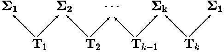
Note that N = kn in an n-cell system with k state variables in each cell. Equivariance of g implies that whenever X(t) is a solution, so is γX(t). Using fixed-point subspaces, Melbourne et al. [7] suggest a method for constructing heteroclinic cycles connecting equilibria. Suppose that Σ ⊂ Γ is a subgroup. Then, the fixed-point subspace:

$$Fix(\mathrm{\Sigma })=\{X\in {\mathbf{R}}^N:\sigma X=X\forall \sigma \in \mathrm{\Sigma }\}$$

is a flow-invariant subspace. The idea is to find a sequence of maximal subgroups Σ_j ⊂ Γ, such that dim Fix(Σ_j) = 1, and submaximal subgroups T_j ⊂ Σ_j ∩ Σ_j+1, such that dim Fix(T_j) = 2, as is shown schematically in Figure 1. In addition, the equilibrium in Fix(Σ_j) must be a saddle in Fix(T_j), whereas the equilibrium in Fix(Σ_j+1) must be a sink in Fix(T_j).

Such configurations of subgroups have the possibility of leading to heteroclinic cycles if saddle-sink connections between equilibria in Fix(Σ_j) and Fix(Σ_j+1) exist in Fix(T_j). It should be emphasized that more complicated heteroclinic cycles can exist. Generally, all that is needed to be known is that the equilibria in Fix(Σ_j) is a saddle and the equilibria in Fix(Σ_j+1) is a sink in the fixed-point subspace Fix(T_j) (see Krupa and Melbourne [8]); although the connections cannot, in general, be proven. Since the saddle-sink connections are robust in a plane, these heteroclinic cycles are stable to perturbations of g, so long as Γ-equivariance is preserved by the perturbation. For a detailed discussion of asymptotic stability and nearly asymptotic stability of heteroclinic cycles, which are also very important topics, see Krupa and Melbourne [8].

Near the points of the Hopf bifurcation, this method for constructing heteroclinic connections can be generalized to include time periodic solutions, as well as equilibria. Melbourne, Chossat and Golubitsky [7] do this by augmenting the symmetry group of the differential equations with S¹, the symmetry group of Poincare–Birkhoff normal form at points of Hopf bifurcation, and using the phase-amplitude equations in the analysis. In these cases, the heteroclinic cycle exists only in the normal form equations, since some of the invariant fixed-point subspaces disappear when symmetry is broken. However, when that cycle is asymptotically stable, then the cycling-like behavior remains, even when the equations are not in the normal form. In later work, Buono, Golubitsky and Palacios [12] proved the existence of heteroclinic cycles involving steady-state and time periodic solutions in differential equations with D_n symmetry.

2.1. The Guckenheimer–Holmes Cycle

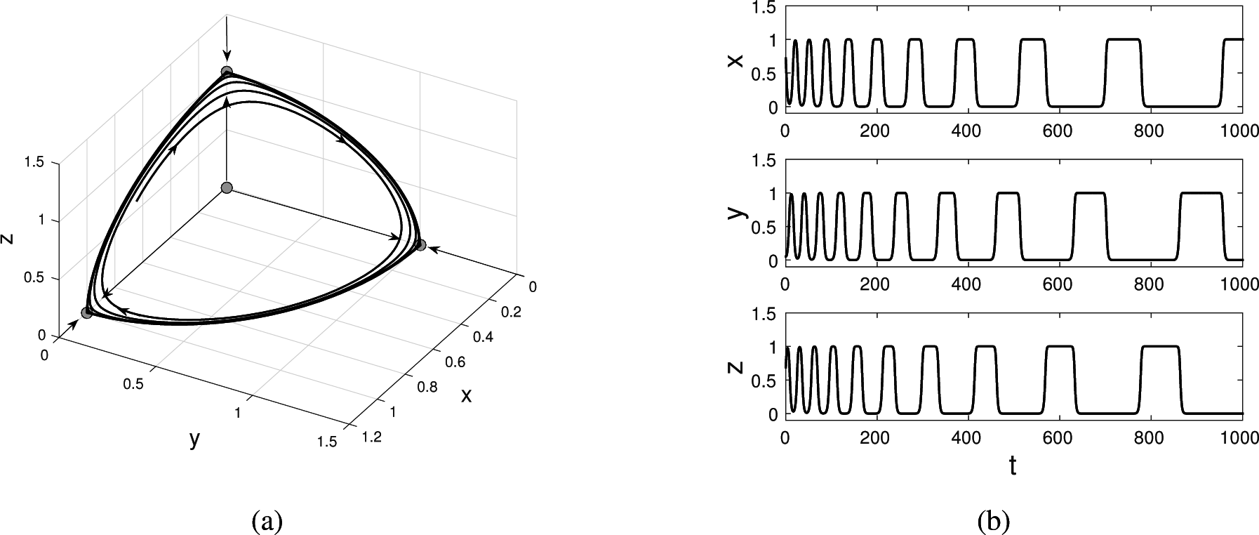
Figure 2 illustrates a cycle involving three steady states of a system of ODEs proposed by Guckenheimer and Holmes [2]. On the left is the phase space. Solid curves depict a solution trajectory right on the invariant manifolds (stable and unstable) of each equilibrium. On the yz-plane, the equilibrium on the z-axis, i.e., (0, 0, z*), is a saddle, while the one on the y-axis, i.e., (0, y*, 0) is a sink. In the absence of any other type of solution on this plane, the Poincare–Bendixson theorem guarantees the existence of a saddle-sink connection. A similar type of saddle-sink connection repeats on each plane, thus leading to a complete cycle. The right side of Figure 2 showcases a time-series evolution of a solution trajectory with initial conditions near the cycle. Observe that as time evolves, the solution trajectory stays longer around each equilibrium.

The group $\Gamma \simeq {\mathbf{Z}}_2^3⋊{\mathbf{Z}}_3$ in this example has 24 elements and is generated by the following symmetries:

$$\begin{array}{l}(x,y,z)\mapsto (\pm x,\pm y,\pm z)\\ (x,y,z)\mapsto (x,y,z).\end{array}$$

Note that, in fact, this is a homoclinic cycle, since the three equilibria are on the group orbit given by the cyclic generator of order three. The actual system of ODEs can be written in the following form:

$$\begin{array}{l}{\dot{x}}_1=\mu x_1-(a{x}_1^2+b{x}_2^2+c{x}_3^2)x_1\\ {\dot{x}}_2=\mu x_2-(a{x}_2^2+b{x}_3^2+c{x}_1^2)x_2\\ {\dot{x}}_3=\mu x_3-(a{x}_3^2+b{x}_1^2+c{x}_2^2)x_3.\end{array}$$

In the related work that describes cycling chaos, Dellnitz et al. [13] point out that the Guckenheimer–Holmes system can be interpreted as a coupled cell system (with three cells) in which the internal dynamics of each cell is governed by a pitchfork bifurcation of the form:

$${\dot{x}}_i=\mu x_i-a{x}_i^3,$$

where i = 1, 2, 3 is the cell number. As µ varies from negative to positive through zero, a bifurcation from the trivial equilibrium x_i = 0 to nontrivial equilibria $x_i=\pm \sqrt{\mu }$ occurs.

Guckenheimer and Holmes [2] show that when the strength of the remaining terms in the system of ODEs (which can be interpreted as coupling terms) is large, an asymptotically-stable heteroclinic cycle connecting these bifurcated equilibria exists. The connection between the equilibria in Cell 1 to the equilibria in Cell 2 occurs through a saddle-sink connection in the x₁x₂-plane (which is forced by the internal symmetry of the cells to be an invariant plane for the dynamics). As Dellnitz et al. [13] further indicate, the global permutation symmetry of the three-cell system guarantees connections in both the x₂x₃-plane and the x₃x₁-plane, leading to a heteroclinic connection between three equilibrium solutions.

3. Cycles in Magnetic and Electric Field Sensor Systems

Overdamped bistable dynamics, of the generic form:

$$\dot{x}=-\nabla U(x),$$

(1)

underpin the behavior of numerous systems in the physical world. In this section, we consider two sensor systems whose dynamics is governed by Equation (1). A fluxgate magnetometer with a potential energy function U(x, t) = x²(t)/2 − c⁻¹ ln(cosh(c(x(t) + h(t)))), and an electric field sensor based on overdamped Duffing systems, with a bistable potential, U(x) = −ax² + bx⁴. Absent an external forcing term, the state-point x(t) in both systems will rapidly relax to one of two stable attractors. Which attractor is observed depends on the particular choice of initial conditions. To follow, a complete description of the system response to an input DC field is presented. The sensitivity of each sensor system is also described in great detail. In particular, it is shown that sensitivity increases significantly near the onset of the heteroclinic connections.

3.1. Magnetic Sensors

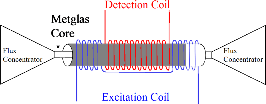
In its most basic form, a fluxgate magnetometer consists of two detection coils wound around a ferromagnetic core (usually a single core) in opposite directions from one another [14,15], as is shown in Figure 3. Fluxgates show bistable dynamics with a hysteresis loop in which the cores can be induced by a bias signal to oscillate between two magnetization states (±1). The dynamics of the magnetizations states is governed by a potential energy function U(x) of the same form as (1). Without an external forcing term, the state point x(t) will rapidly relax to one of two stable attractors, which are the minima of the potential energy function U(x). This behavior leads to the standard, spectral-based [14,16,17] detection mechanism of small target signals (DC or low frequency), wherein a known periodic bias signal is applied to induce the sensor to oscillate between its two stable attractors. In the absence of a target signal, the power spectral density contains only the odd harmonics of the bias frequency. In the presence of a weak target signal, however, the potential energy function is skewed, resulting in the appearance of even harmonics; the response at the second harmonic is then used to detect and quantify the target signal. The drawbacks of this readout mechanism are: (1) it requires a great amount of onboard power to provide a high-amplitude, high-frequency bias signal; (2) the feedback electronics can introduce their own noise floor into the measurement process; and (3) high-amplitude, high-frequency bias signals often increase the noise floor of the system. Fluxgates were originally developed about 1928 for use as a submarine detection device for low-flying aircraft. Today, individual highly-specialized fluxgate devices can measure magnetic fields in the range of 1–10 $\mathrm{pT}/\sqrt{Hz}$ [18,19], and they are used in applications, such as: geophysical exploration, surveillance in land and sea and underwater exploration [20–23].

One must, however, take these performance quantifiers with the caveat that, when operated unshielded in a practical application, the detection of target signals above the noise floor is limited by the ambient magnetic field (which, in the case of the terrestrial magnetic field, can have non-stationary, as well as random components). Hence, various techniques often involving a reference magnetometer for the purposes of subtraction of the noise floor from the output of the target-sensing device must be employed if one wishes to take advantage of the low noise floor. Among recent advances in fluxgate sensor technology, the so-called “fluxset” devices [24] (see also [15,17,25] for good overviews), which differ from a conventional fluxgate in the way they convert the magnetic field into an output electrical signal, are noteworthy. The fluxset magnetometer is based on the influence of the external magnetic field on the time necessary to produce the reversal magnetization of the ferromagnetic core under a periodic magnetic excitation. Given an optimal core design and excitation field, the time shift depends only on the value of the external (target) magnetic field. Hence, the measurement of the magnetic field amplitude via a voltage measurement in the fluxgate is replaced by a high accuracy time measurement that can be rendered more impervious to clutter signals and noise via an understanding of the device response in the presence of a noise floor. Such a (deterministic) “time-domain” description was first introduced by Strycker and Wulkan [26].

3.2. Modeling

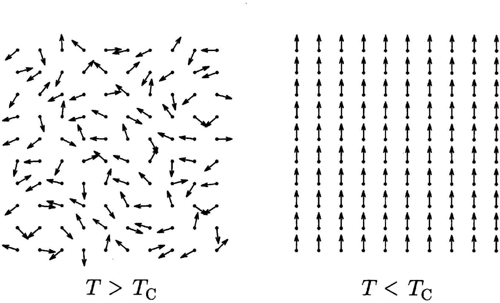
A simple way to model the ferromagnetic core dynamics in a fluxgate is through an Ising-type model. We will assume the core to be composed of a set of atomic “spins” arranged on a regular lattice representing the crystal structure of the core [27]. When the temperature T exceeds a critical temperature T_c, called the Curie temperature, the system exhibits a phase transition [28,29] from a paramagnet state with little magnetization properties to a ferromagnetic state, where magnetization is uniform; see Figure 4.

A further simplification is to consider spin 1/2 magnetic materials, so that only two distinct orientations at each lattice point i are possible: “up” (S_i = +1) or “down” (S_i = −1). Then the average magnetic field h_i at spin S_i is determined by adding the average contributions from all neighboring spins S_j and from any external applied field h^ext through Glauber dynamics [30],

$$\langle h_i\rangle ={\displaystyle \sum _{j\to i}{w}_{ij}}\langle S_j\rangle +h^{ext},Prob(S_i=\pm 1)=\frac{1}{1+\exp (\mp 2\beta h_i)},$$

where w_ij is the coupling strength of the influence of spin S_j on S_i and β is related to the temperature T through β = 1/(k_BT ), where k_B is Boltzmann’s constant. Direct calculations show that the average magnetization is given by 〈S_i〉 = tanh (β〈h_i〉) = tanh (β∑w_ijh〈S_j〉 + βh^ext). Our interest is in the ferromagnetic state, in which 〈S_i〉 = 〈S〉. Assuming identical coupling strengths w_ij = 1/N, where N is the number of spins, we find a single equation for the average magnetization: 〈S〉 = tanh (β〈S〉+βh^ext). An extension of this equation with continuous updating of the average magnetization state leads to a simple continuous model of the fluxgate core dynamics:

$$\tau \frac{dx}{dt}=-x+\tanh \left(\frac{x+h}{T}\right)\equiv -\frac{\partial U(x)}{\partial x},$$

(2)

where τ is a relaxation parameter, x = 〈S〉, k_B = 1, so that β = 1/T is a pseudo-temperature parameter, h = h^ext, and U(x) is the energy function U(x) = x²/2 − T ln(cosh((x + h)/T)).

The model Equation (2) for a conventional fluxgate magnetometer can be rewritten, after rescaling time, as a nonlinear dynamical system of the form:

$$\dot{x}=-x+\tanh (c(x+A\sin \omega t+\in )),$$

(3)

where x represents the magnetization state of the core, c is a temperature-related parameter, A is the amplitude of the biasing signal with frequency ω and ε is the external magnetic field to be detected. In the absence of a biasing signal, i.e., A = 0, and without an external signal, i.e., ε = 0, the system dynamics will quickly settle into one of two equilibrium points of (3). For a sufficiently large biasing signal, however, the system may be induced to oscillate.

3.3. Network Architecture

A coupled-core fluxgate magnetometer (CCFM) is then constructed by uni-directionally coupling N (odd) wound ferromagnetic cores with cyclic boundary conditions [6], thereby leading to the dynamics,

$${\dot{x}}_i=-x_i+\tanh (c(x_i+\lambda x_{i+1}+\in )),i=1,\dots ,N\mathrm{mod}N,$$

(4)

where x_i(t) represents the (suitably normalized) magnetic flux at the output (i.e., in the secondary coil) of unit i and ε ≪ U₀ is an external DC “target” magnetic flux, U₀ being the energy barrier height (absent the coupling) for each of the elements (assumed identical for theoretical purposes); the parameter λ represents the strength of coupling between x_i and x_i+1. Effectively, the unidirectional coupling leads to a network with Z_N-symmetry, where Z_N is the cyclic group of permutations of N objects. This network symmetry is critical in the creation of a heteroclinic cycle and, more importantly, in the accompanying infinite-period bifurcations of limit cycle oscillations.

Indeed, a bifurcation analysis [3,6] reveals that the system (4) displays oscillatory behavior with the following features:

• The oscillations commence when the coupling coefficient exceeds a threshold value:

  $${\lambda }_c=-\epsilon -x_{inf}+c^{-1}{\tanh }^{-1}{x}_{inf},$$

  (5)
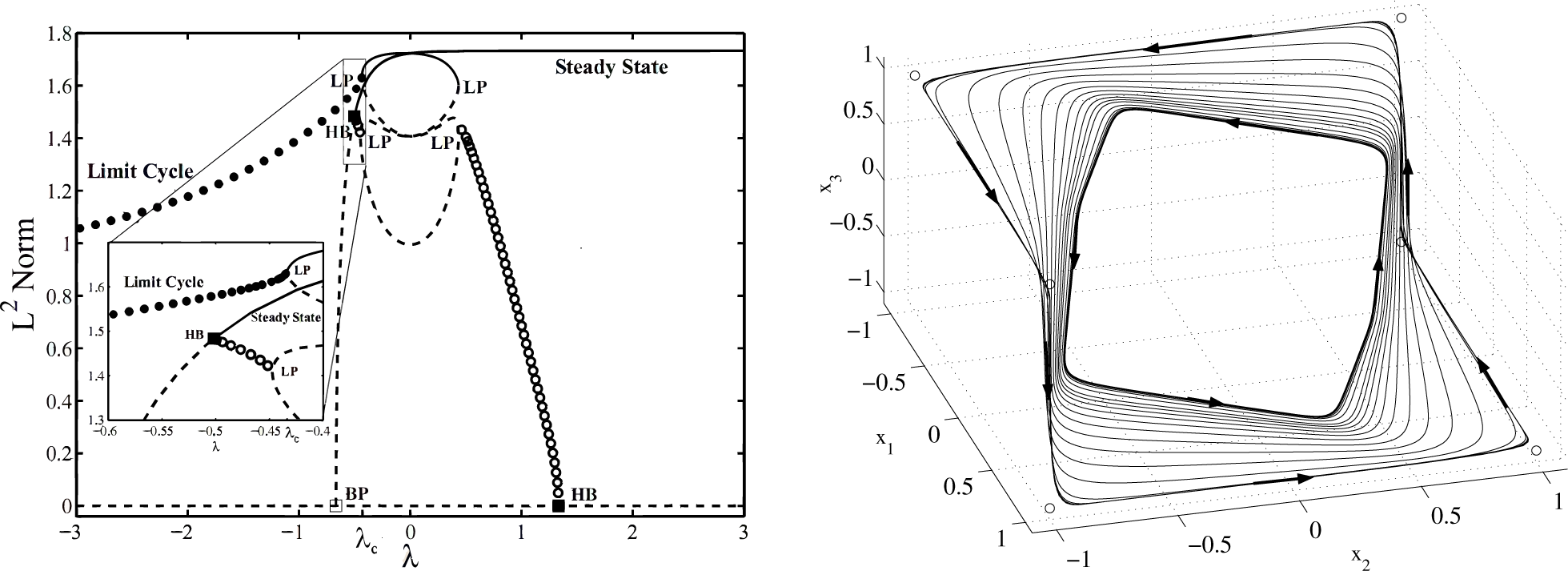
  with $x_{inf}=\sqrt{(c-1)/c}$. Note that in our convention, λ < 0 (negative feedback), so that oscillations occur for |λ| > |λ_c|. The oscillations are non-sinusoidal, with a frequency that increases as the coupling strength decreases away from λ_c. For λ > λ_c, however, the system quickly settles into one of its steady states, regardless of the initial conditions. The same result ensues if N is even or if the coupling is bidirectional. For values of λ slightly less than λ_c, there is a small interval λ_HB ≤ λ ≤ λ_c where global oscillations and synchronous equilibria of the form $(x_1,\dots ,x_N)=(\overline{x},\dots ,\overline{x})$ can coexist; see the two paragraphs below for a more in-depth description.

  The bifurcation diagram for the N = 3 case is shown in Figure 5. It was generated with the aid of the continuation package AUTO [31]. Filled-in circles represent stable oscillations; they emerge via an infinite-period global bifurcation that coincides with the creation of a heteroclinic cycle that connects multiple saddle-point equilibria.

  At the birth of the oscillations, the amplitudes are fully grown due to the global nature of the bifurcation. As λ approaches λ_c (from the left), so that the strength of the negative feedback is reduced, the oscillation period lengthens and finally becomes infinite at λ = λ_c, when the heteroclinic cycle appears. Empty circles describe unstable oscillations; they all appear via local Hopf bifurcations (labeled HB), so their amplitude increases as a square-root law of the distance from the bifurcation point. Solid (dotted) lines depict stable (unstable) equilibrium points. In particular, the equilibrium points that appear at the pitchfork bifurcation point, labeled B, are all synchronous, i.e., of the form $(x_1,x_2,x_3)=(\overline{x},\overline{x},\overline{x})$. A close-up view of the interval of the bistability of large amplitude oscillations and stable synchronous equilibria is also included. The four branches of unstable equilibria that appear via saddle-node bifurcations (labeled LP) correspond to non-synchronous equilibria. Collectively, there are fifteen equilibrium points: three synchronous equilibria, including the trivial solution, and twelve non-synchronous equilibrium points.

• The individual oscillations (in each elemental response) are separated in phase by 2π/N and have period:

  $$T_i=\frac{N\pi }{\sqrt{c{x}_{inf}}}\left(\frac{1}{\sqrt{{\lambda }_c-\lambda }}+\frac{1}{\sqrt{{\lambda }_c-\lambda +2\epsilon }}\right),$$

  (6)
  which shows a characteristic dependence on the inverse square root of the bifurcation “distance” λ_c − λ, as well as the target signal ε. These oscillations can be experimentally produced at frequencies ranging from a few Hz to high kHz.

• The summed output oscillates at period T₊ = T_i/N, and its amplitude (as well as that of each elemental oscillation) is always a suprathreshold, i.e., the emergent oscillations are strong enough to drive the core between its saturation states, eliminating the need to apply an additional bias signal for this purpose, as is done in single-core magnetometers. Increasing N changes the frequency of the individual elemental oscillations, but the frequency of the summed response is seen to be independent of N.

3.4. Magnetic-Field Sensitivity

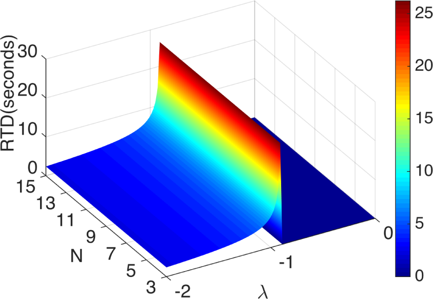
To measure an external signal, we rely on a readout mechanism: the residence times detection (RTD), which is based on a threshold crossing strategy of measuring the symmetry-breaking effect of an external signal. More specifically, RTD consists of measuring the “residence times” of the oscillations of the sensor device about the two stable states of the potential energy function U(x). In the absence of noise and of external signals, the potential energy function is symmetric; hence, the two residence times are identical, i.e., T₊ = T₋. In the presence of a target signal, however, the hysteresis loop is skewed, and the crossing times are no longer equal. Then, either the difference |T₊ − T₋| or the ratio T₊/T₋ of residence times can be used to quantify the signal. In the presence of noise, the residence times must be replaced by their ensemble averages. The advantages of this procedure are: it can be implemented on-chip without the computationally-demanding power spectra of the system output; large-period oscillations yield large differences/ratios of residence times, i.e., better sensitivity; and it can be optimized to require very low onboard power. This mechanism is much more sensitive than standard techniques based on the power spectra decomposition, because the long period of oscillations that are characteristic of limit cycles near the onset of a heteroclinic connection renders their wave form highly sensitive to symmetry breaking effects. Direct computations [4] show that RTD can be calculated as:

$$\mathrm{\Delta }t\approx \frac{\pi (1/\sqrt{{\lambda }_c-\lambda }-1/\sqrt{{\lambda }_c-\lambda +2\epsilon })}{\sqrt{c{x}_{inf}}},$$

(7)

which vanishes (as expected) for ε = 0, and can be used as a quantifier of the target signal, analogous to the time-domain operation of the single fluxgate.

The system responsivity, defined via the derivative ∂Δt/∂ε, is found to increase dramatically as one approaches the critical point in the oscillatory regime; see Figure 6. This suggests that careful tuning of the coupling parameter so that the oscillations have very low frequency could offer significant benefits for the detection of very small target signals.

For small target signals, one may do a small-ε expansion to yield:

$$\mathrm{\Delta }t\approx \frac{\pi }{\sqrt{c{x}_{inf}}}\left[\frac{1}{\sqrt{{\lambda }_{c3}-\lambda }}-\frac{1}{\sqrt{{\lambda }_{c3}-\lambda +2\epsilon }}\right],$$

where λ_c3 now represents the critical coupling obtained using the signal from x₃ as a reference point. Further details can be found in [4]. For a fixed ε, one observes, immediately, that the responsivity ∂Δt/∂ε increases as one approaches the critical point (through adjusting the coupling parameter λ). The instrument thus yields its optimal performance in the very low frequency regime, close to the oscillation threshold; it is worth noting that the experimental system can be made to oscillate at very low frequencies (around 65 Hz), far lower than the bias frequency for conventional fluxgates. The coupled system can be “tuned” to this regime by adjusting the coupling coefficient λ.

3.5. Alternating Configuration

Laboratory experiments seem to indicate that the sensitivity of a CCFM-based system of fluxgates increases by simply alternating the orientation of each individual fluxgate [4]. We call this new arrangement a CCFM system with alternating orientation (AO). We should clarify that the coupling scheme remains the same, i.e., unidirectional coupling via induction. The only feature that changes is the direction at which the individual fluxgates are aimed for signal detection purposes. Thus, the sign in front of the target signal ε alternates between + and −, so that the governing equations (for the deterministic system) become,

$${\dot{x}}_i=-x_i+\tanh (c(x_i+\lambda x_i+{(-1)}^{i+1}\epsilon )),i=1,\dots ,NmodN.$$

(8)

In the absence of noise and of a target signal, i.e., ε = 0, Equation (8) reduces to that of the standard CCFM system (4). Hence, the one-parameter bifurcation of x_i vs. λ remains the same: the coupling-induced oscillations exist only when N is odd and for $\lambda <{\lambda }_c^{AO}$, where ${\lambda }_c^{AO}$ is a critical threshold value of coupling strength and the superscript denotes the type of configuration. The two-parameter bifurcation of x_i vs. (λ, ε) might be, however, different, since the signs in front of the input signal are now different. Thus, we seek to determine ${\lambda }_c^{AO}$ as a function of ε. Direct calculations yield:

$${\lambda }_c^{AO}=-\in +\frac{1}{c}\ln (\sqrt{c}+\sqrt{c-1})-\tanh (\ln (\sqrt{c}+\sqrt{c-1})),$$

(9)

which is exactly the same value obtained in Equation (12) for the standard configuration. Interestingly, the AO configuration does not change the two-parameter region where stable coupling-induced oscillations exist. More interesting, however, is the fact that the sensitivity response of the AO configuration does change. Actually, it improves significantly:

$${\mathrm{\Delta }}^{AO}t\approx \frac{N\pi }{\sqrt{c{x}_{inf}}}\left[\frac{1}{\sqrt{{\lambda }_{c3}-\lambda }}-\frac{1}{\sqrt{{\lambda }_{c3}-\lambda +2\epsilon }}\right].$$

It follows that:

$$\frac{\partial {\mathrm{\Delta }}^{AO}t}{\partial \epsilon }=N\frac{\partial \mathrm{\Delta }t}{\partial \epsilon }.$$

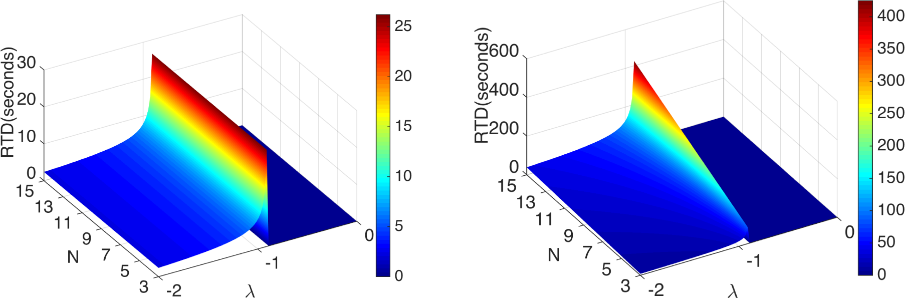
In other words, the sensitivity of the AO configuration improves, linearly, by a factor of N when it is compared to the best sensitivity that can be achieved by the summed output signal of the standard configuration, given the same external signal and core parameters. The dependence of the RTD, and consequently of the sensitivity, on the size of the ring in the AO configuration is in direct contrast to the sensitivity response of the standard configuration, in which increasing N beyond N = 3 does not lead to additional benefits. We should emphasize that the standard configuration, nevertheless, still outperforms the sensitivity of a magnetometer based on a single uncoupled core. The above observations are confirmed in Figure 7, in which we calculate, numerically, the RTD Δ₁t for a CCFM system with the standard, as well as with the AO configuration.

3.6. Robustness

We expect noise in a coupled-core fluxgate magnetometer network to arise from three sources: a magnetic noise floor (due to the core material and, in particular, magnetic domain motion), contamination of the target signal and noise from the electronics in the coupling circuitry. In recent work, we studied, numerically, the effects of an additive magnetic noise floor [32] and of a target signal contaminated by noise. In both cases, we assumed Gaussian band-limited noise having zero mean, correlation time τ_c and variance σ². This type of noise is a good approximation (except for a small 1/f component at very low frequencies) to what is actually observed in the experimental setup. From a modeling point of view, colored noise η(t) that contaminates the signal should appears now as an term inside the tanh function of Equation (4), while additive noise is simply added to the tanh function, i.e.,

$$\begin{array}{l}\frac{d{x}_i}{dt}=-x_i\tanh (c(x_i+\lambda x_{i+1}+\epsilon +{\eta }_i(t)))+{\xi }_i(t)\\ \frac{d{\eta }_i}{dt}=-\frac{{\eta }_i}{{\tau }_c}+\frac{\sqrt{2D}}{{\tau }_c}\xi (t)\\ \frac{d{\nu }_i}{dt}=-\frac{{\nu }_i}{{\tau }_c}+\frac{\sqrt{2D}}{{\tau }_c}\xi (t).\end{array}$$

(10)

In general, we would expect somewhat different noise in each equation, since, realistically, the reading of the external signal ε is slightly different in each core. This is due to non-identical circuit elements and cores, mainly. In this work, we will consider, therefore, the situation wherein the the different noise terms η_i(t) and ν_i are uncorrelated; however, for simplicity, we will assume them to have the same intensity D. Each (colored) noise η_i(t) is characterized by 〈η_i(t)〉 = 0 and 〈η_i(t)η_i(s)〉 = (D/τ_c)×exp [−|t − s|/τ_c], where $D={\sigma }^2{\tau }_c^2/2$ is the noise intensity, and the “white” limit is obtained for vanishing τ_c. Similar expressions apply to ν_i(t). In practice, however, the noise is always band-limited. In this formulation, we assume the signal to be contaminated purely by external noise; in future work, however, we will also consider other sources of contamination, such as internal noise introduced by each individual core, as well as the coupling and readout circuits.

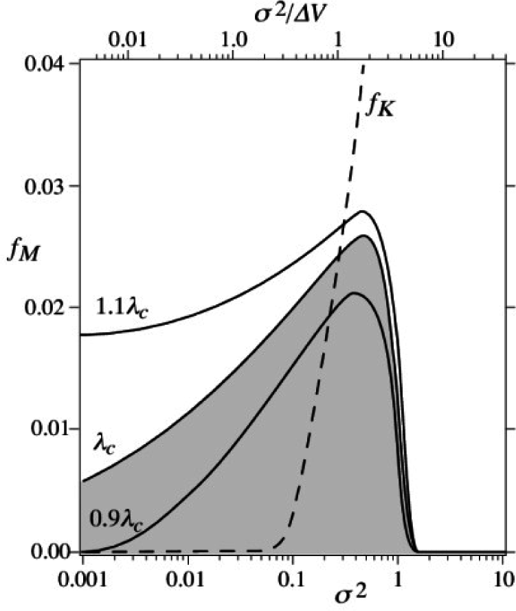
We now present first the results from the numerical simulations of the coupled system (10) in the presence of additive, Gaussian, band-limited white noise. For convenience, the nonlinearity parameter c is also taken to be the same throughout. Further, we consider only the case of zero target signal (i.e., ε = 0), so that the system is a priori symmetric. The power spectral density (PSD) of any of the solutions x_i(t) shows interesting features. Specifically, it appears to share much in common with what is observed in renewal processes [33]. Given the near-instantaneous transition between the upper and lower thresholds, preceded by a relatively slow transition to the threshold (this is readily observable in the deterministic time series) and coupled with the (not unreasonable) assumption of independent crossing events, the renewal description seems to be a good one. The features of the PSD are better explained with reference to Figure 8, which shows the modal switching frequency (the location, f_M, of the fundamental peak in the corresponding PSD) of a single element in the N = 3 ring, as a function of the noise intensity for two values of the coupling coefficient bracketing its critical value. In this figure, we also plot (for comparison purposes) the characteristic (Kramers) noise-induced hopping rate, which is numerically computed for a single uncoupled element in the spectral amplitude occurring at zero frequency for large noise. For the suprathreshold case, we have, already, a deterministic oscillation frequency, and the effect of the noise is to replace this spike with a broad (and shifted) peak and its odd (because the system is symmetric) harmonics. For very small noise intensities, the modal oscillation frequency (i.e., the inverse mean of the period distribution function) does not deviate appreciably from the deterministic oscillation frequency; this is also evident in the top curve of Figure 8, wherein one observes a finite oscillation frequency even for zero noise, as expected. With increasing noise intensity, however, the mean oscillation frequency becomes a function of the noise and separates itself from the deterministic frequency. Simultaneously (with increasing noise), the peak amplitude (in the PSD) decreases until, past the Kramers rate f_K, the PSD has its maximum amplitude at zero frequency (for any value of λ), as would be expected. The occurrence of hopping events in the subcritical regime, where the deterministic system is quiescent, is, clearly, a case of purely noise-induced switching.

Finally, we address the issue of increasing the number of elements in the coupled array. Changing N leads to a proportionate scaling of the individual frequencies of the component elements; however, the summed output oscillates at a frequency independent of N. Increasing N also leads to an enhancement in the spectral response of individual elements in the array, but not for the summed output.

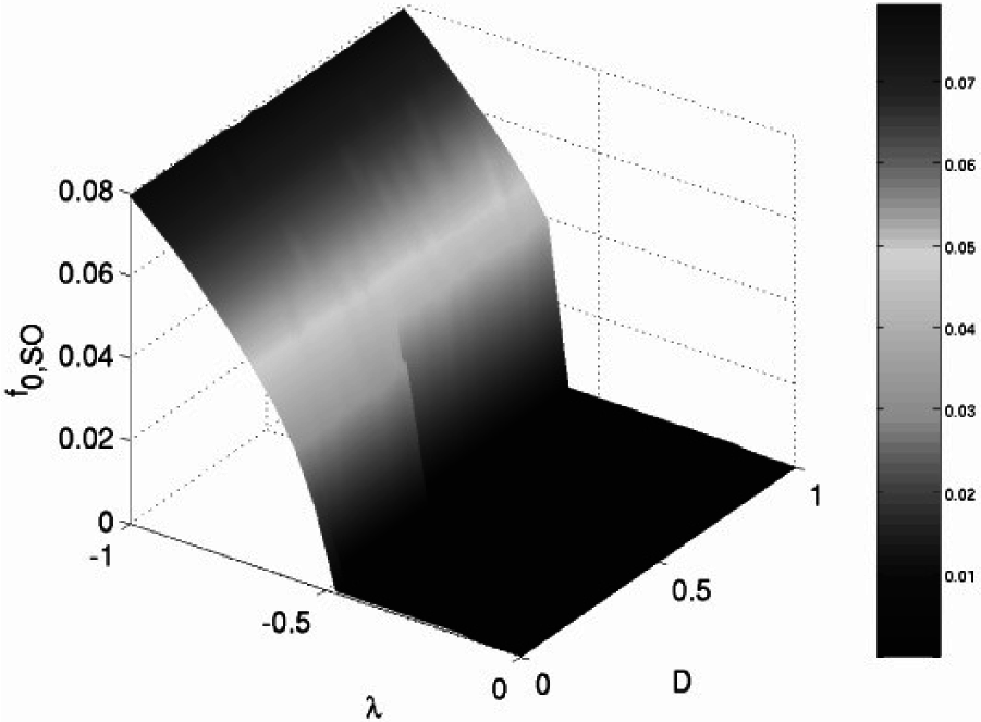
We now consider the effects of signal contamination by noise. We assume the temperature-related parameter c to be constant throughout the simulations. We assume the target signal to be ε = 0.07, well below the energy threshold of a single (uncoupled) core. Of course, the results are expected to be similar to those found at other values of the target signal within the energy barrier height. Figure 9 shows the relation between the mean oscillation frequency of (a single core element of) the CCFM with N = 3 cores and the system parameters (coupling strength λ and noise intensity D). The mnemonic “SO” in the figure stands for standard orientation, in which all of the individual cores have the same spatial orientation (i.e., the sign of the target signal term is the same in each equation of the system Equation (10)) for signal detection purposes. A sample of one thousand time-series simulations was then used to compute the frequency output at each point in the parameter space (λ, D). Each simulation was carried out with correlation time set to τ_c = 150, since typically τ_F ≪ τ_c, where τ_F = 1 is the time constant of the core dynamics given by Equation (4). Observe that the critical-coupling bifurcation point λ_c of the deterministic system, i.e., D = 0, remains, approximately, unchanged for small values of noise intensity. There is, however, a subtle shift in the bifurcation point for increasing noise (beyond D = 0.25). The noise appears to have the effect of delaying the onset of oscillatory behavior. We find (not shown) that the delay is less pronounced in the more idealized scenario in which the noise η_i(t) is taken to be the same in each core.

Next, we study the response of the CCFM through the signal-to-noise ratio (SNR). Figure 10 shows the SNR (of the output of a single core element) in the same parameter space (λ, D). The SNR increases rapidly near the critical coupling, as we would expect. The negative effects of highly-contaminated signals (large noise intensity) appear to be well mitigated by the sensitivity response of the system. To the right of the onset of oscillatory behavior, where the global dynamics of the deterministic system typically settle into a steady-state equilibrium, we now observe small fluctuations in the SNR caused mainly by noise. These fluctuations get smaller as the number of simulation samples increases.

It is worth mentioning that these small fluctuations are also present in the more ideal case, wherein we take identical noise functions in each element of the dynamics. We now investigate the AO configuration, which, as suggested by the results of the preceding section, as well as our laboratory experiments, holds the promise of further performance enhancements.

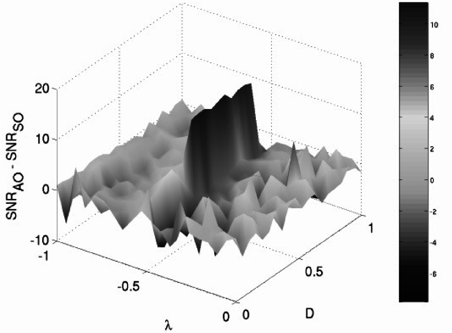
Finally, we study the effects of noise on the CCFM with the AO configuration. We use the output of the “favored” element that gives the best deterministic RTD response (see the preceding section) in this configuration. Calculations of the SNR output of this “favored” element (not shown for brevity) show, at first glance, similar results to those of the standard-orientation configuration. A point-wise comparison between the SNR output of the two cases indicates, however, that the SNR output of (the favored element of) the AO configuration can be larger than that of the standard (CCFM) system (Figure 11). Near the critical coupling strength, in particular, the SNR response of the AO system appears to be significantly better than that of the standard configuration. Large coupling strengths, on the contrary, reduce the SNR response of the AO configuration to values that are comparable to those of the standard case. The improvement in SNR output of the AO configuration over the standard (SO) case is also present in the ideal case of identical noises in the cores; however, in this case, the improvement occurs for smaller values of noise intensity. In both cases, non-identical and identical noise terms, the difference between the SNR outputs suggests that careful tuning of the coupling strength can mitigate the negative effects of signal contamination, so that full advantage can be taken of the sensitivity enhancements of a CCFM system with the AO configuration.

3.7. Basins of Attraction

Modeling and analysis of high-dimensional dynamical systems is usually focused on finding conditions for the existence and stability of typical invariant sets, i.e., steady states, periodic solutions and chaotic sets. High dimensionality leads to complex patterns of collective behavior. Which behavior is exhibited by a network depends greatly on the initial conditions. Thus, it is also important to study the geometric structure and evolution of the basins of attraction of such patterns. In this section, we provide a qualitative description of the equilibrium points of the unidirectionally-coupled ring of fluxgate magnetometers with governing Equation (4). In particular, we emphasize the role of the network symmetry, defined by the group Z_N, in the multiplicity of the various equilibrium points. For illustration purposes, we focus the description on the particular case of N = 3. The derivatives are set equal to zero, and the nonlinear system of equations is solved to find the equilibria. It is apparent that the origin (0,0,0) is one equilibrium point independent of λ. However, all other equilibria are found using numerical methods. In addition, we need the eigenvalues and eigenvectors from the linearization about the equilibria, which uses the Jacobian of the RHS of System (4):

$$J(x_1,x_2,x_3;\lambda )=\left(\begin{array}{ccc}-1+c{\text{sech}}^2((c(x_1+\lambda x_2))& c\lambda {\text{sech}}^2((c(x_1+\lambda x_2))& 0\\ 0& -1+c{\text{sech}}^2((c(x_2+\lambda x_3))& c\lambda {\text{sech}}^2((c(x_2+\lambda x_3))\\ c\lambda {\text{sech}}^2((c(x_3+\lambda x_1))& 0& -1+c{\text{sech}}^2((c(x_3+\lambda x_1))\end{array}\right).$$

There are a number of methods for finding the many equilibria for System (4). Perhaps the most efficient way is with the aid of the software packages AUTO [31] and XPPAUT [34]. From the known equilibrium at the origin, AUTO can track equilibria and periodic orbits, as it finds bifurcation points by varying λ, which give rise to new equilibria. For System (4), the easiest way to find and track equilibria is to start with the case λ = 0, the uncoupled system. Then, equilibria are found by solving:

$$-x_1+\tanh (c{x}_i)=0,$$

which, for c = 3, gives x_ie = 0 being unstable and x_ie = ±0.9949 being stable in the x_i direction. For System (4) at λ = 0, there are 27 equilibria from all possible combinations of the three equilibria for each of the three components. Furthermore, the information on the stability of each component transfers to the entire system. It follows that there are eight stable nodes from all combinations of:

$$(x_{1e},x_{2e},x_{3e})=(\pm 0.9949,\pm 0.9949,\pm 0.9949).$$

The origin is clearly an unstable node. The equilibria with one component, x_ie = 0, and the other two components having x_je = ±0.9949, j ≠ i, produce twelve unstable saddle nodes with 2D stable manifolds. These 2D stable manifolds align with the coordinate planes in each of the octants. Finally, there are six unstable saddle nodes with two components satisfying x_ie = 0 and the remaining one having x_je = ±0.9949. These equilibria have 1D stable manifolds along the coordinate axes.

With these equilibria established for System (4) with λ = 0, the fsolve routine in MATLAB is used in a program to find the equilibria for other λ. The fsolve routine uses a Levenberg–Marquardt method to solve the vector system:

$$\mathbf{F}(\mathbf{x},\lambda )=0,$$

for x. One of the equilibria above is used as initial conditions, then λ is varied slowly in the positive and negative directions over the desired domain or until a saddle node bifurcation is encountered. At each step of the procedure for computing new equilibria, the new value of λ is entered with the previously-computed equilibrium value used as an initial guess. MATLAB’s fsolve routine can readily find a new equilibrium, unless we are very close to a saddle node bifurcation. If we are close to a saddle node bifurcation, then the stepsize of λ is reduced to obtain the new equilibrium value. If the initial equilibrium, (x_1e, x_2e, x_3e), is an asynchronous equilibrium point, then symmetry automatically produces five more equilibria: (x_2e, x_3e, x_1e), (x_3e, x_1e, x_2e), (−x_1e, −x_2e, −x_3e), (−x_2e, −x_3e, −x_1e) and (−x_3e, −x_1e, −x_2e). Furthermore, all six of these equilibria maintain the properties, like the unstable saddle node with a 2D stable manifold, which agree with the properties of the initial equilibrium at λ = 0. These properties are easily checked at any equilibrium by finding the eigenvalues of the Jacobian matrix, J(x_1e, x_2e, x_3e; λ), at the equilibrium.

Even though there are 27 equilibria, there are only six qualitatively different ones. The eight stable equilibria divide into two categories with the two symmetric equilibria and the six asymmetric equilibria. There are twelve asymmetric equilibria with 2D stable manifolds, which also divide into two categories. The first six are the ones that, when λ = 0, border on the faces of Octant I or its negative, Octant VII, generating the lavender separatrices, and the other six come from the remaining equilibria on the faces of the other octants when λ = 0, generating the green separatrices. Finally, the six equilibria on the coordinate axes when λ = 0 generate the equilibria with 1D stable manifolds. Figure 12 shows the evolution of these different types of equilibria as λ varies. The origin remains a fixed, unstable equilibrium with some of its eigenvalues changing sign only at the point of the pitchfork bifurcation (λ = −0.6667) and the subcritical Hopf (λ = 1.3333). Consider first the two symmetric equilibria, and recall the 24-element group $\Gamma \simeq {\mathbf{Z}}_2^3⋊{\mathbf{Z}}_3$ of symmetries of the coupled bistable system. Reflections send one of the symmetric equilibria (x, x, x) to the other (−x, −x, −x), and vice versa, while cyclic rotations leave them unchanged. In other words, the pair of symmetric equilibria are in the group orbit generated from the symmetry group $\Gamma \simeq {\mathbf{Z}}_2^3⋊{\mathbf{Z}}_3$. Thus, from a symmetry standpoint, these two equilibria are one and the same. Upon changing λ, the group orbit evolves while it tracks the line x₁ = x₂ = x₃, starting at λ = −0.6667, and both equilibria on the orbit become stable (as expected, because they are in the same group orbit) after the subcritical Hopf bifurcation at λ = −0.5018. The resulting equilibria are visible as the straight-line segment shades from gray to black in the middle of Figure 12.

Figure 12 also shows that the asymmetric stable equilibria track six small curves remaining near the points:

$$\langle 1,1,-1\rangle \to \langle -1,1,-1\rangle \to \langle -1,1,1\rangle \to \langle -1,-1,1\rangle \to \langle 1,-1,1\rangle \to \langle 1,-1,-1\rangle .$$

Similarly, these equilibria are symmetrically related and share stability properties, since they are in the same (second) group orbit generated by Γ. The small curves track from gray to black as λ ∈ (−0.4346, 0.4346) varies. The gray end of the curve connects to one set of six equilibria with 2D stable manifolds, which are shown in Figure 12, starting with the lighter blue and becoming darker as λ ∈ (−0.4346, 0.4349) varies. This particular set generates the green 2D stable manifolds in our previous figures, and when λ = 0, these curves pass through a point (x_1e, x_2e, x_3e), where the x_ie, i = 1, 2, 3 is a permutation of the values −0.9949, 0 and 0.9949. The permutation is equivalent to applying the 24-elements of the symmetry group Γ, which yields a total of 12 asymmetric unstable nodes connected in a third group orbit. The dark end of these six blue curves matches the dark end of the six red curves at the saddle node bifurcation when λ = 0.4349. The six red curves sweep a long arc passing through one of the coordinate axes near x_ie = ±0.9949 for some i = 1, 2, 3, where six additional unstable saddle nodes are located. These six saddle node points form the fourth group orbit of equilibria. As the red becomes lighter, these curves reach another saddle node bifurcation at λ = −0.4475, where they match with the light end of the other set of six blue curves. This set of six blue curves of equilibria have 2D stable manifolds, which are lavender in the previous figures, separating the symmetric equilibria from the asymmetric equilibria. When λ = 0, these equilibria are on one of the coordinate planes with two values of x_ie being either ±0.9949 and the other being x_je = 0. These six curves become darker as λ increases to 0.4346, where the lavender stable manifolds vanish at a saddle node bifurcation. This saddle node bifurcation has the dark blue curve match the black of another asymmetric stable equilibrium at a different adjacent corner. The evolution of the stable and unstable manifolds is shown in Figure 13 through a montage of the geometric structure of the basins of attraction. More details can also be found in [35].

In summary, the 24 asymmetric equilibrium points can be arranged into one of three distinct group orbits. Thus, Figure 12 can be interpreted as a color-coded evolution of four distinct group orbits as a function of λ, which yields: a straight-line in the middle connecting the two symmetric equilibria (±x, ±x, ±x) and the origin; six gray-to-black corner segments connecting six asymmetric stable nodes of the form (±x, ±x, ∓x); twelve blue curves for the group orbit of twelve asymmetric unstable nodes with representative (0, ±x, ±x); six red curves, which connect the remaining six asymmetric unstable saddle nodes of the type (0, 0, ±x). All other equilibria can be readily obtained by applying directly the 24 elements of the group Γ to the representative elements listed above. We observe in Figure 12 that if one begins at any one of the asymmetric equilibria and increases and decreases λ between the saddle node bifurcation values, then one can continuously reach all of the remaining 23 asymmetric equilibria. This property deserves further investigation. The codes used to generate these equilibria are available at [36].

3.8. Electric Field Sensor

We consider a system of N (unidirectionally) coupled bistable overdamped Duffing elements, in the presence of a weak (compared to the energy barrier height of a single uncoupled element) DC external target signal ε₀:

$$\tau {\dot{x}}_i=a{x}_i-b{x}_i^3+\lambda (x_i-x_{i+1})+{\epsilon }_0,$$

(11)

where i = 1, …, N mod N, x_i(t) is a generic state variable, with the parameters (a, b) characterizing each element, λ being an inter-element coupling coefficient (note the absence of bidirectional coupling) and c a coupling constant (or amplification parameter, depending on the mechanism) to the external target signal. τ is a time constant, usually depending in a complex way on geometrical and physical (material) parameters; it defines (via its inverse) the individual element bandwidth. One realizes, immediately, that the dynamics of the system (11) are likely to be quite different from the magnetic sensors discussed in Section 3.1 because of the differences in the (inter-element, as well as external signal) coupling mechanisms.

A bifurcation analysis [5] reveals that the system (11) exhibits oscillatory behavior with the following features:

• The oscillations commence when the coupling coefficient exceeds a threshold value:

  $${\lambda }_c={\lambda }_{c0}+\frac{3}{2}\frac{{\epsilon }_0}{1+\sqrt{\frac{2a}{b}}},$$

  (12)
  to leading order in ε₀. This expression for the critical coupling is found to agree quite well with the results of numerical simulations on the coupled system (11), for small ε₀ (compared to the energy barrier height U₀). As was the case of the coupled magnetic sensors, the oscillations are again non-sinusoidal, with a frequency that increases as the coupling strength increases away from λ_c. For λ < λ_c, however, the system quickly settles into one of its steady states, regardless of the initial conditions. The same result ensues if N is even or if the coupling is bidirectional. The bifurcation diagram for the N = 3 case is shown in Figure 14. Again, it was generated with the aid of the continuation package AUTO [31]. Filled-in circles represent stable oscillations; they emerge via an infinite-period global bifurcation that coincides with the creation of a heteroclinic cycle that connects multiple saddle-point equilibria. Empty circles represent unstable oscillations. Observe that they appear via local Hopf bifurcations, marked with an H. Solid (dotted) lines represent branches of stable (unstable) equilibrium points. For values of λ slightly larger than λ_c, there is a small interval where global oscillations and synchronous equilibria of the form $(x_1,\dots ,x_N)=(\overline{x},\dots ,\overline{x})$ can coexist.

• The individual oscillations (in each elemental response) are separated in phase by 2π/N and have period:

  $$T=\frac{3\sqrt{2\pi }}{\sqrt{\left|f(x_{10})f^{″}(x_{10})\right|}}+\frac{3\sqrt{2\pi }}{\sqrt{\left|f(x_{30})f^{″}(x_{30})\right|}},$$

  (13)
  where $f(x)=(a+\lambda )x_1-b{x}_1^3-\lambda x_{2m}+{\epsilon }_0,x_{10}=\sqrt{\frac{a+\lambda }{3b}},x_{30}=-x_{10}$.

• Increasing N leads to a concomitant increase in the individual oscillation periods, but the period of the summed response is independent of N.

3.9. Electric-Field Sensitivity

The residence time difference in the two states is easily evaluated, via the summed response, as:

$$\mathrm{\Delta }t=\frac{\sqrt{2\pi }}{\sqrt{\left|f(x_{10})f^{″}(x_{10})\right|}}-\frac{\sqrt{2\pi }}{\sqrt{\left|f(x_{30})f^{″}(x_{30})\right|}},$$

note that the quantity Δt would incorporate a factor of N if we evaluated it for each individual element. We also point out that, unlike in our previous work [6], it does not appear possible to (analytically) obtain a clear-cut scaling behavior of the period T with the “separation” Δλ ≡ λ − λ_c from the expressions above; in fact, the necessity to recourse to Taylor expansions for the steady-state quantities x_i0, as well as the critical coupling λ_c attests to the calculational difficulties associated with this (seemingly straightforward, especially in comparison to the more complicated mean-field potential energy functions of [6]) coupled system (11), even near the critical point.

4. Experiments

Figure 15 shows an actual realization of a CCFM with three fluxgate magnetometers coupled unidirectionally. The PCB (printed circuit board) version is made of cobalt-based Metglas 2714A material, and each is sandwiched between two sheets of PCB material. The sides of the PCB sheets that face away from the core material are printed with copper wiring to form the windings for the driving and sensing coils. Solder is used to fuse the two sheets together to complete the circuit for the windings. The cores are then coupled through electronic circuits where the (voltage) readout of one fluxgate signal (i.e., the derivative signal of the flux detected by the sensing coil) is amplified by a voltage amplifier with a very high impedance, which also trims out any DC signal in the output; see Figure 16. Following this, the signal is passed through a “leaky” integrator to convert the derivative signal seen by the sensing coil back to the “flux” form, so that the experimental system closely conforms to the model (4).

Typically, the integrator output contains a DC component that must be removed before the signal is passed to the other fluxgates. This is accomplished by employing a Sallen–Key second-order high pass filter immediately after the integrator. The signal then passes through an amplifier to achieve adequate gain to drive the adjacent fluxgate. After this, the signal passes through a voltage-to-current converter (V-I converter) in its final step to drive the primary coil of the adjacent fluxgate. The setup repeats for the remaining two fluxgates, and all values of the coupling circuit parameters are closely matched from one set to the other.

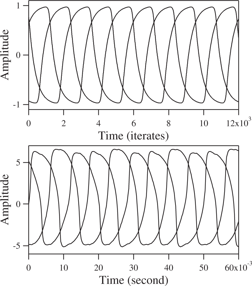
The oscillations observed from this setup are quite striking; see Figure 17. The system readily oscillates in a traveling pattern. Like the model, the system favors this pattern no matter how many times it is restarted. The frequency of oscillations is about 33.5 Hz. Each wave is phase shifted by exactly $\frac{2\pi }{3}$, as predicted by the model. Comparison of the oscillations from the experiment to the numerical results shows good agreement. In addition, since we do not know the value of c and the time constant τ in the actual device (we set τ = 1 in the model), we cannot correctly compare the time scales in the model and the experimental observations. The amplitudes of the oscillations in the experiment are also arbitrary compared to the model, because the recorded voltages depend on the gains set in the coupling circuit. On the other hand, the magnetic flux in the model saturates between ±1, but in the fluxgate devices, this quantity cannot be measured directly.

5. Conclusions

Over the past twelve years, we have conducted various analytical, computational and experimental works to investigate the fundamental idea that coupling-induced oscillations that emerge through heteroclinic connections can be exploited to develop a new generation of highly-sensitive, low-powered, dynamic sensors. In this review article, we use the fluxgate magnetometer, which is essentially a coil sensor with a ferromagnetic core, and a network of electric field sensors made up of overdamped Duffing oscillators as case studies to illustrate the basic ideas and methods to enhance sensor performance. Both sensor systems are coupled in a ring configuration with no preferred orientation, i.e., uni-directionally. This type of coupling configuration favors the existence of structurally-stable heteroclinic cycles that involve saddle-sink connections between multiple equilibrium points. More importantly, the cycles are accompanied by a branch of globally-stable limit cycle oscillations. At birth, these oscillations are fully grown with a large amplitude, which distinguishes them from the slowly-growing oscillations that emerge via Hopf bifurcations. This is a critical feature to enhance performance, because the large period, large amplitude oscillations that typically occur near the onset of a heteroclinic connection render the collective oscillations highly sensitive to symmetry-breaking effects caused by external signals. An experimental prototype of a network of fluxgate magnetometers yields voltage oscillations that are in very good agreement with computer simulations of the model equations. More importantly, the sensitivity of the device is significantly stronger than that of a single unit, as expected.

In more recent years, we have expanded the ideas and methods to model, analyze and develop highly sensitive sensor systems beyond magnetic- and electric-field sensors. In particular, we have extensively studied networks of vibratory gyroscopes for navigation systems. Current prototype MEMS (micro-electro-mechanical systems) gyroscopes are compact and inexpensive to produce, but their performance characteristics, in particular drift rate, fail to meet the requirements for an inertial grade guidance system. As an alternative approach, a coupled inertial navigation sensor, made up of N vibratory gyroscopes coupled in some fashion, has been proposed [37–41]. The fundamental idea is to synchronize the motion of each gyroscope to the Coriolis driving force, so that the collective signal from all gyroscopes can be summed and then demodulated to yield an optimal response in terms of minimizing phase drift and robustness to noise and material imperfections. An analysis (based on perturbation methods) with N = 3 gyroscopes shows promising results, as the coupled system appears to minimize phase drift. The governing equations for larger array sizes are, however, not amenable to similar analysis based on perturbation techniques. This lack of tractability prevent us from exploring further performance enhancements in phase drift by larger arrays. To circumvent this problem, in recent projects, we have reformulated the governing equations in a Hamiltonian structure, and the corresponding normal forms are then derived [42]. Through a normal form analysis, we can investigate the effects of various coupling schemes and unravel the nature of the bifurcations that lead a ring of gyroscopes of any size into and out of synchronization. The Hamiltonian approach can, in principle, be readily extended to other symmetry-related systems. Future work includes translational research work aimed at the design and fabrication of a prototype system at both the mesoscale and microscale.

In yet another project at the interface between symmetric dynamical systems and engineering, we have also shown a proof of concept that an array of vibratory energy harvesters, coupled mechanically and inductively, can produce, under certain conditions that depend mainly on the coupling strength, collective patterns of oscillations [43]. Among the many different patterns, synchronization behavior is of particular importance, because, in principle, it can be used to form a coherent power output to a usable level to drive some devices. A perturbation analysis shows that it is possible to find approximate analytical expressions for the critical coupling strength that leads to the stable synchronized solutions. The analysis is, however, complicated for it to be extended to arrays of arbitrary size, specially large arrays. An alternative approach, based on casting the model equations in Hamiltonian form, with zero forcing and zero damping, leads to an approximate analytical solution for the onset of synchronization. The expression is a reasonable approximation, even under weak forcing, and it can be very useful towards the design and operation of an array of energy harvesters for higher combined energy production. In the analysis, we chose the model equations representing the energy harvester constructed with magnetostrictive material, as a case study. However, we wish to emphasize that the fundamental principles of symmetry-driven spatio-temporal patterns of oscillations are model independent, so that similar ideas of arrays of harvesters can be readily extended to other arrays with different materials, for instance piezoelectric transduction. Finally, we note that power production has not been discussed at this point, because the entire experimental system is not fully optimized yet to give a realistic projection of the total power production from the coupled system. The optimization will be carried out mainly in the power converter part where the impedance matching, component sizes and load matching are very important to efficiently convert power to do useful work. We plan to discuss this part of the system in a future work.

References

- Field, M. Equivariant dynamical systems. Trans. Am. Math. Soc. 1980, 259, 185–205. [Google Scholar]
- Guckenheimer, J.; Holmes, P. Structurally stable heteroclinic cycles. Math. Proc. Camb. Philos. Soc. 1988, 103, 189–192. [Google Scholar]
- Bulsara, A.; In, V.; Kho, A.; Longhini, P.; Palacios, A.; Rappel, W.; Acebron, J.; Baglio, S.; Ando, B. Emergent oscillations in unidirectionally coupled overdamped bistable systems. Phys. Rev. E. 2004, 70, 036103. [Google Scholar] [CrossRef]
- Palacios, A.; Aven, J.; In, V.; Longhini, P.; Kho, A.; Neff, J.; Bulsara, A. Coupled-core fluxgate magnetometer: Novel configuration scheme and the effects of a noise-contaminated external signal. Phys. Lett. A. 2007, 367, 25–34. [Google Scholar]
- In, V.; Palacios, A.; Bulsara, A.; Longhini, P.; Kho, A.; Neff, J.; Baglio, S.; Ando, B. Complex Behavior in Driven Unidirectionally Coupled Overdamped Duffing Elements. Phys. Rev. E. 2006, 73, 066121. [Google Scholar] [CrossRef]
- In, V.; Bulsara, A.; Palacios, A.; Longhini, P.; Kho, A.; Neff, J. Coupling induced oscillations in overdamped bistable systems. Phys. Rev. E. 2003, 68, 045102. [Google Scholar] [CrossRef]
- Melbourne, I.; Chossat, P.; Golubitsky, M. Heteroclinic cycles involving periodic solutions in mode interactions with O(2) symmetry. Proc. Roy. Soc. Edinb. 1989, 113A, 315–345. [Google Scholar]
- Krupa, M.; Melbourne, I. Asymptotic stability of heteroclinic cycles in systems with symmetry. Ergod. Theory Dyn. Syst. 1995, 15, 121–147. [Google Scholar]
- Field, M. Lectures on Bifurcations, Dynamics and Symmetry; Pitman Research Notes in Mathematics; Addison-Wesley Longman Ltd.: Harlow, UK, 1996; Volume 356. [Google Scholar]
- Krupa, M. Robust heteroclinic cycles. J. Nonlin. Sci. 1997, 7, 129–176. [Google Scholar]
- Krupa, M. Bifurcations of relative equilibrias. SIAM J. Math. Anal. 1990, 21, 1453–1486. [Google Scholar]
- Buono, P.L.; Golubitsky, M.; Palacios, A. Heteroclinic cycles in rings of coupled cells. Phys. D. 2000, 143, 74–108. [Google Scholar]
- Dellnitz, M.; Field, M.; Golubitsky, M.; Ma, J.; Hohmann, A. Cycling chaos. Int. J. Bifurc. Chaos. 1995, 5, 1243–1247. [Google Scholar]
- Ripka, P. Review of fluxgate sensors. Sens. Actuators A. 1996, 33, 129–141. [Google Scholar]
- Ripka, P. Advances in fluxgate sensors. Sens. Actuators A. 2003, 106, 8–14. [Google Scholar]
- Primdahl, F. Fluxgate Magnetometers. In Bibliography of Fluxgate Magnetometers; Publications of the Earth Physics Branch, Department of Energy, Mines and Resources: Ottawa, Canada, 1970; Volume 41. [Google Scholar]
- Ripka, P. New directions in fluxgate sensors. J. Magn. Magn. Mater. 2000, 215–216, 735–739. [Google Scholar]
- Karlsson, M.; Robinson, J.; Gammaitoni, L.; Bulsara, A. The optimal achievable accuracy of the Advanced Dynamic Fluxgate Magnetometer (ADFM). Proceedings of the 3rd International Conference on Marine Electromagnetics (MARELEC), Stockholm, Sweden, 11–13 July 2001.
- Koch, R.; Deak, J.; Grinstein, G. Fundamental limits to magnetic-field sensitivity of flux-gate magnetic-field sensors. Appl. Phys. Lett. 1999, 75, 3862–3864. [Google Scholar]
- Gordon, D.; Brown, R. Recent advances in fluxgate magnetometry. IEEE Trans. Magn. 1972, 8, 76–82. [Google Scholar]
- Lenz, J. A Review of Magnetic Sensors. IEEE Proc. 1990, 78, 973–989. [Google Scholar]
- Russell, C.; Elphic, R.; Slavin, J. Initial Pioneer Venus magnetic field results: Dayside observations. Science 1979, 203, 745–748. [Google Scholar]
- Snare, R.; Means, J. A magnetometer for the Pioneer Venus mission. IEEE Trans. Magn. 1997, 13, 1107–1977. [Google Scholar]
- Vertesy, G.; Szollosy, J.; Varga, L.K.; Lovas, A. High sensitivity magnetic field sensors using amorphous alloy. Electron. Horiz. 1992, 53, 102. [Google Scholar]
- Ripka, P. Noise and stability of magnetic sensors. J. Magn. Magn. Mater. 1996, 157–158, 424–427. [Google Scholar]
- Strycker, S.; Wulkan, A. A pulse position type fluxgate magnetometer. AIEE Trans 1961, 80, 253–257. [Google Scholar]
- Brailsford, F. Magnetic Materials; John Wiley & Sons, Inc: New York, NY, USA, 1951. [Google Scholar]
- Bertotti, G. Hystersis in Magnetism; Academic Press: San Diego, CA, USA, 1998. [Google Scholar]
- Stanley, H. Introduction to Phase Transitions and Critical Phenomena; Oxford University Press: Oxford, UK, 1971. [Google Scholar]
- Glauber, R. Time-Dependent statistics of the Ising model. J. Math. Phys. 1963, 4, 294–307. [Google Scholar]
- Doedel, E.; Wang, X. Auto94: Software for Continuation and Bifurcation Problems in Ordinary Differential Equations; Applied Mathematics Report; California Institute of Technology: Pasadena, CA, USA, 1994. [Google Scholar]
- Bulsara, A.; Lindner, J.; In, V.; Kho, A.; Baglio, S.; Sacco, V.; Ando, B.; Longhini, P.; Palacios, A.; Rappel, W. Coupling-Induced cooperative behavior in dynamic ferromagnetic cores in the presence of noise. Phys. Lett. A. 2006, 353, 4–10. [Google Scholar]
- Lukes, T. Space Correlation and Energy Levels in an Einstein Solid dagger. Proc. Phys. Soc. 1961, 78. [Google Scholar] [CrossRef]
- Ermentrout, B. Simulating, Analyzing, and Animating Dynamical Systems: A Guide to Xppaut for Researchers and Students; Society for Industrial and Applied Mathematics (SIAM): Philadelphia, PA, USA, 2002. [Google Scholar]
- Lyons, D.; Mahaffy, J.; Wang, S.; Palacios, A.; In, V. Geometry of basins of attraction and heteroclinic connections in coupled bistable systems. Int. J. Bif. Chaos. 2014, 24, 1430029. [Google Scholar] [CrossRef]
- Lyons, D.; Mahaffy, J.; Wang, S.; Palacios, A.; In, V. Computer Code for the Computational and Visualization of Basins of Attraction, Available online: http://www.rohan.sdsu.edu/antoniop/research/ accessed on 19 June 2015.
- Davies, N.; Vu, H.; Palacios, A.; In, V.; Longhini, P. Collective behavior of a coupled gyroscope system with coupling along the drive and sense modes. Int. J. Bifurc. Chaos. 2013, 23. [Google Scholar] [CrossRef]
- Davies, N. Ring of VIbratory Gyroscopes with Coupling Along the Drive and Sense Axes. Master’s Thesis, San Diego State University, San Diego, CA, USA, 2011. [Google Scholar]
- Vu, H. Ring of Vibratory Gyroscopes with Coupling along the Drive Axis. Ph.D. Thesis., San Diego State University, San Diego, CA, USA, 2011. [Google Scholar]
- Vu, H.; Palacios, A.; In, V.; Longhini, P.; Neff, J. A drive-free vibratory gyroscope. Chaos 2011, 21, 013103. [Google Scholar] [CrossRef]
- Vu, H.; Palacios, A.; In, V.; Longhini, P.; Neff, J. Two-time scale analysis of a ring of coupled vibratory gyroscopes. Phys. Rev. E. 2010, 81, 031108. [Google Scholar] [CrossRef]
- Buono, P.; Chan, B.; Palacios, A.; In, V. Dynamics and bifurcations in a Dn symmetric Hamiltonian network with applications to coupled gyroscopes. Phys. D. 2015, 290, 8–23. [Google Scholar]
- Matus-Vargas, A.; Gonzalez-Hernadez, H.; Chan, B.; Palacios, A.; Buono, P.; In, V.; Naik, S.; Phipps, A.; Longhini, P. Dynamics, Bifurcations and Normal Forms in Arrays of Magnetostrictive Energy Harvesters with All-to-All Coupling. Int. J. Bifurc. Chaos. 2015, 25, 1550026. [Google Scholar] [CrossRef]
© 2015 by the authors; licensee MDPI, Basel, Switzerland This article is an open access article distributed under the terms and conditions of the Creative Commons Attribution license (http://creativecommons.org/licenses/by/4.0/).
Share and Cite
Palacios, A.; In, V.; Longhini, P. Symmetry-Breaking as a Paradigm to Design Highly-Sensitive Sensor Systems. Symmetry 2015, 7, 1122-1150. https://doi.org/10.3390/sym7021122
Palacios A, In V, Longhini P. Symmetry-Breaking as a Paradigm to Design Highly-Sensitive Sensor Systems. Symmetry. 2015; 7(2):1122-1150. https://doi.org/10.3390/sym7021122
Chicago/Turabian StylePalacios, Antonio, Visarath In, and Patrick Longhini. 2015. "Symmetry-Breaking as a Paradigm to Design Highly-Sensitive Sensor Systems" Symmetry 7, no. 2: 1122-1150. https://doi.org/10.3390/sym7021122