
Dynamical Symmetries and Causality in Non-Equilibrium Phase Transitions

Groupe de Physique Statistique, Institut Jean Lamour (CNRS UMR 7198), Université de Lorraine Nancy, B.P. 70239, F-54506 Vandoeuvre-lès-Nancy Cedex, France
Symmetry 2015, 7(4), 2108-2133; https://doi.org/10.3390/sym7042108
Submission received: 10 July 2015
/
Revised: 28 October 2015
/
Accepted: 29 October 2015
/
Published: 13 November 2015
(This article belongs to the Special Issue Lie Theory and Its Applications)
Abstract
:Dynamical symmetries are of considerable importance in elucidating the complex behaviour of strongly interacting systems with many degrees of freedom. Paradigmatic examples are cooperative phenomena as they arise in phase transitions, where conformal invariance has led to enormous progress in equilibrium phase transitions, especially in two dimensions. Non-equilibrium phase transitions can arise in much larger portions of the parameter space than equilibrium phase transitions. The state of the art of recent attempts to generalise conformal invariance to a new generic symmetry, taking into account the different scaling behaviour of space and time, will be reviewed. Particular attention will be given to the causality properties as they follow for co-variant n-point functions. These are important for the physical identification of n-point functions as responses or correlators.
1. Introduction
Improving our understanding of the collective behaviour of strongly interacting systems consisting of a large number of strongly interacting degrees of freedom is an ongoing challenge. From the point of view of the statistical physicist, paradigmatic examples are provided by systems undergoing a continuous phase transition, where fluctuation effects render traditional methods such as mean-field approximations inapplicable [1,2]. At the same time, it turns out that these systems can be effectively characterised in terms of a small number of “relevant” scaling operators, such that the net effect of all other physical quantities, the “irrelevant” ones, merely amounts to the generation of corrections to the leading scaling behaviour. From a symmetry perspective, phase transitions naturally acquire some kind of scale-invariance, and it then becomes a natural question whether further dynamical symmetries can be present.
1.1. Conformal Algebra
In equilibrium critical phenomena (roughly, for systems with sufficiently short-ranged, local interactions), scale-invariance can be extended to conformal invariance. In two space dimensions, the generators should obey the infinite-dimensional algebra
for . The action of these generators on physical scaling operators , where complex coordinates are used, is conventionally given by the representation [3]
and similarly for , where the rôles of z and are exchanged. Herein, the conformal weights are real constants, and related to the scaling dimension and the spin of the scaling operator ϕ. The representation Equation (2) is an infinitesimal form of the (anti)holomorphic transformations and . The maximal finite-dimensional sub-algebra of Equation (1) is isomorphic to . It is this conformal sub-algebra only which has an analogue in higher space dimensions . Denoting the Laplace operator by , the conformal invariance of the Laplace equation is expressed through the commutator
and analogously for . Hence, for vanishing conformal weights and , any solution of is mapped onto another solution of the same equation. Thermal fluctuations in classical critical points or quantum fluctuations in quantum critical points (at temperature ) modify the conformal algebra Equation (1) to a pair of commuting Virasoro algebras, parametrised by the central charge c. Then Equation (2) retains its validity when the set of admissible operators ϕ is restricted to the set of primary scaling operators (a scaling operator is called quasi-primary if the transformation Equation (2) only holds for the finite-dimensional sub-algebra ) [4]. In turn, this furnishes the basis for the derivation of conformal Ward identities obeyed by n-point correlation functions of primary operators . Celebrated theorems provide a classification of the Virasoro primary operators from the unitary representations of the Virasoro algebra, for example through the Kac formula for central charges [5,6]. Novel physical applications are continuously being discovered.
1.2. Schrödinger Algebra
When turning to time-dependent critical phenomena, the theory is far less advanced. One of the best-studied examples is the Schrödinger–Virasoro algebra in d space dimensions [7,8]
(all other commutators vanish) with integer indices , half-integer indices and . Casting the generators of into the four families makes explicit (i) that the generators form a conformal sub-algebra and (ii) that the families and make up Virasoro primary operators of weight and 1, respectively [7]. Non-trivial central extensions are only possible (i) either in the conformal sub-algebra , where it must be of the form of the Virasoro central charge, or else (ii) in the -current algebra , where it must be a Kac–Moody central charge [5,6,7,9]. The maximal finite-dimensional sub-algebra of is the Schrödinger algebra , where is central. An explicit representation in terms of time-space coordinates , acting on a (scalar) scaling operator of scaling dimension x and of mass , is given by [7]
with the abbreviations and . These are the infinitesimal forms of the transformations , where
where is an arbitrary time-dependent function, is a non-decreasing function and denotes a rotation matrix with time-dependent rotation angles. The generators do not generate a time-space transformation, but rather produce a time-dependent “phase shift” of the scaling operator ϕ [10].
The dilatations are the infinitesimal form of the transformations and , where is a constant and z is called the dynamical exponent. In the representation Equation (5), one has .
Since the work of Lie [12], and before of Jacobi [13], the Schrödinger algebra is known to be a dynamic symmetry of the the free diffusion equation (and, much later, also of the free Schrödinger equation). Define the Schrödinger operator
Following Niederer [14], dynamical symmetries of such linear equations are analysed through the commutators of with the symmetry Lie algebra. For the case of , the only non-vanishing commutators with are
Hence, any solution ϕ of the free Schrödinger/diffusion equation with scaling dimension is mapped onto another solution of the free Schrödinger equation [15]. Finally, from representations such as Equation (5), one can derive Schrödinger–Ward identities in order to compute the form of covariant n-point functions . With respect to conformal invariance, one has the important difference that the generator is central in the finite-dimensional non-semi-simple Lie algebra . This implies the Bargman super-selection rule [17]
Physicists’ conventions require that “physical masses” . It it therefore necessary to define a formal “complex conjugate” of the scaling operator ϕ, such that its mass becomes negative. Then one may write, e.g., a non-vanishing co-variant two-point function of two quasi-primary scaling operators (up to an undetermined constant of normalisation) [7]
Here and throughout this paper, if and if . While Equation (10) looks at first sight like a reasonable heat kernel, a closer inspection raises several questions:
- Why should it be obvious that the time difference , to make the power-law prefactor real-valued ?
- Given the convention that , the condition is also required in order to have a decay of the two-point function with increasing distance .
- In applications to non-equilibrium statistical physics, one studies indeed two-point functions of the above type, which are then interpreted as the linear response function of the scaling operator ϕ with respect to an external conjugate fieldwhich in the context of the non-equilibrium Janssen–de Dominicis theory [2] can be re-expressed as a two-point function involving the scaling operator ϕ and its associate response operator . In this physical context, one has a natural interpretation of the “complex conjugate” in terms of the relationship of ϕ and .Then, the formal condition simply becomes the causality condition, namely that a response will only arise at a later time after the stimulation at time .
Hence, it is necessary to inquire under what conditions the causality of Schrödinger-covariant n-point functions can be guaranteed.
1.3. Conformal Galilean Algebra
Textbooks in quantum mechanics show that the Schrödinger equation is the non-relativistic variant of relativistic wave equations, be it the Klein–Gordon equation for scalars or the Dirac equations for spinors. One might therefore expect that the Schrödinger algebra could be obtained by a contraction from the conformal algebra, but this is untrue (although there is a well-known contraction from the Poincaré algebra to the Galilei sub-algebra). Rather, applying a contraction to the conformal algebra, one arrives at a different Lie algebra, which we call here the altern-Virasoro algebra [11,18,19,20]. with , but which nowadays is often referred to as infinite conformal Galilean algebra. Its non-vanishing commutators can be given as follows
An explicit representation as time-space transformation is [21]
where is a vector of dimensionful constants, called rapidities, and x is again a scaling dimension. The dynamical exponent . The maximal finite-dimensional sub-algebra of is the conformal Galilean algebra [11,18,22,23,24,25,26,27].
A more abstract characterisation of can be given in terms of α-densities , with the action
Lemma 1. [33] One has the isomorphism, where ⋉ denotes the semi-direct sum
Clearly, it follows that .
As before, the time-space representation Equation (13) can be used to derive conformal-Galilean Ward identities. For example, the -covariant two-point function takes the form
Again, at first sight this looks physically reasonable, but several questions must be raised:
- Why should one have for the time difference, as required to make the power-law prefactor real-valued ?
- Even for a fixed vector of rapidities, and even if could be taken for granted, how does one guarantee that the scalar product , such that the two-point function decreases as ?
The finite-dimensional admits a so-called “exotic” central extension [34,35]. Abstractly, this is achieved by completing the commutators Equation (12) by the following
with a central generator Θ. This is called the exotic Galilean conformal algebra in the physics literature. A representation as time-space transformation of ecga is, with and [21,24,36]
The components of the vector satisfy , where θ is a constant, ε is the totally antisymmetric tensor and [37]. The dynamical exponent . Because of Schur’s lemma, the central generator Θ can be replaced by its eigenvalue . The ecga-invariant Schrödinger operator is
with . The requirement that these representations should be unitary gives the bound [24]. Co-variant n-point functions and their applications have been studied in great detail.
1.4. Ageing Algebra
The common sub-algebra of and is called the ageing algebra with and does not include time-translations. Starting from the representation Equation (5), only the generators assume a more general form [38]
such that is kept from Equation (5). When the generator is applied to a scaling operator, the constant ξ describes a second scaling dimension, besides the habitual one denoted here by x, of that scaling operator ϕ. It is an important new aspect of extended dynamical symmetries, far from a stationary state, that at least two distinct scaling dimensions of a given scaling operator ϕ must be introduced. This will be made explicit later through concrete examples.
The invariant Schrödinger operates now becomes , but without any constraint, neither on x nor on ξ [39]. Co-variant n-point functions can be derived as before [1,38,40], but we shall include these results with those to be derived from more general representations in the next sections. The absence of time-translations is particular appealing for application to dynamical critical phenomena, such as physical ageing, in non-stationary states far from equilibrium, see [1].
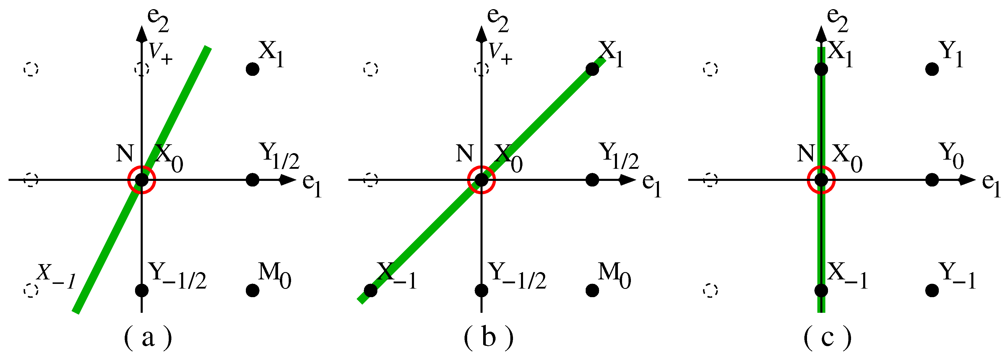
In Figure 1 (on page 19 below), the root diagrammes [41] of the Lie algebra (a) , (b) and (c) are shown, where the generators (roots) are represented by the black dots. This visually illustrates that the Schrödinger and conformal Galilean algebras are not isomorphic, .
Comparing Figure 1a with Figure 1c, a different representation of can be identified. This representation is spanned by the generators from Equation (5), along with a new generator , and leads to a dynamic exponent [11]. It is not possible to extend this to a representation of [33]. Explicit expressions of will be given in Section 4.
1.5. Langevin Equation and Reduction formulæ
In non-equilibrium statistical mechanics [2], one considers often equations under the form of a stochastic Langevin equation, viz. (we use the so-called “model-A” dynamics with a non-conserved order-parameter)
for a physical field ϕ (called the order parameter), and where stands for a functional derivative. Herein, is the Ginzburg–Landau potential and η is a white noise, i.e., its formal time-integral is a Brownian motion. In the context of Janssen–de Dominicis theory, see [2], this can be recast as the variational equation of motion of the functional
where the term contains the deterministic terms coming from the Langevin equation and contains the stochastic terms generated by averaging over the thermal noise and the initial condition, characterised by an initial correlator [43]. In particular, by adding an external source term to the potential , one can write the two-time linear response function as follows (spatial arguments are suppressed for brevity)
with an explicit expression of the average as a functional integral.
Theorem 1. [44] If in the functional , the part is Galilei-invariant with non-vanishing masses and does not contain the field ϕ, then the computation of all responses and correlators can be reduced to averages which only involve the Galilei-invariant part .
Proof. We illustrate the main idea for the calculation of the two-time response. Define the average with respect to the functional . Then, from Equation (23)
since the Bargman super-selection rule Equation (9) implies that only the term with remains. Hence the response function is reduced to the expression obtained from the deterministic part of the action.
Analogous reduction formulæ can be derived for all Galilei-covariant n-point responses and correlators [1,44]. ☐
This means that one may study the deterministic, noiseless truncation of the Langevin equation and its symmetries, provided that spatial translation- and Galilei-invariance are included therein, in order to obtain the form of the stochastic two-time response functions, as it will be obtained from models, simulations or experiments.
This work is organised as follows. In Section 2, we review several distinct representations of the Schrödinger and conformal Galilean algebras, discuss the associated invariant Schrödinger operators an co-covariant two-point functions. Applications to non-equilibrium statistical mechanics and the non-relativistic AdS/CFT correspondence will be indicated. In Section 3, the dual representations and the extensions to parabolic sub-algebras will be reviewed. In Section 4, it will be shown how to use these, to algebraically derive causality and long-distance properties of co-variant two-point functions. Conclusions are given in Section 5.
2. Representations
We now list several results relevant for the extension of the representations discussed in the introduction. The basic new fact, first observed in [40], is compactly stated as follows.
Proposition 1. Let γ be a constant and a non-constant function. Then the generators
obey the conformal algebra for all .
The commutator is readily checked. We point out that the rapidity γ serves as a second scaling dimension and the choice of the function can be helpful to include effects of corrections to scaling into the generators of time-space transformations. Next, we give an example on how these terms in the generators appear in the two-point function, co-variant under the maximal finite-dimensional sub-algebra .
Proposition 2. If is a quasi-primary scaling operator under the representation Equation (24) of the conformal algebra , its co-variant two-point function is, where is a normalisation constant
Proof. For brevity, denote . Then the co-variance of F is expressed by the three Ward identities, with
Rewrite the correlator as . Then the function satisfies
which are the standard Ward identities of the representation Equation (2) of conformal invariance, where the take the rôle of the conformal weights. The resulting function Ψ is well-known [45]. ☐
One can now generalise the representation Equation (5) of the Schrödinger–Virasoro algebra .
Proposition 3. If one replaces in the representation Equation (5) the generator as follows
where are constants and is an arbitrary (non-constant) function, then the commutators Equation (4) of the Lie algebra are still satisfied.
This result was first obtained, for the maximal finite-dimensional sub-algebra , by Minic, Vaman and Wu [40], who also further take the dependence on the mass into account and write down terms of order and in explicitly. We extend this observation to , but do not trace the dependence in explicitly, although one could re-introduce it, if required. The proof is immediate, since all modifications of the generator merely depend on the time t and none of the other generators of changes t. For the sub-algebra , the representation Equation (20) is a special case, with arbitrary ξ, but with .
It is obvious that similar extensions of the representations of time-space transformation of the other algebras, especially , its finite-dimensional sub-algebra or the exotic algebra apply.
Proposition 4. Consider the representation Equation (5), but with the generators replaced by Equation (26), of the ageing algebra and the Schrödinger algebra . The invariant Schrödinger operator has the form
such that a solution of is mapped onto another solution of the same equation. For the algebra , there is no restriction, neither on x, nor on ξ, nor on . For the algebra , one has the additional condition .
Proof. To shorten the calculations, we restrict here to . It is enough to restrict attention to the generators , and we must reproduce Equation (8) in this more general setting. We first look at . Consideration of gives and considering gives , where the dot denotes the derivative with respect to t. The second relation can be simplified to which gives the assertion. Going over to , the condition leads to . This is only compatible with the result found before for , if , hence , as claimed. ☐
Example 1. For a physical illustration of the meaning of the explicitly time-dependent terms in the Schrödinger operator Equation (27), we consider the growth of an interface [46]. One may imagine that an interface can be created by randomly depositing particle onto a substrate. The height of this interface will be described by a function . One usually works in a co-moving coordinate system such that the average height which we shall assume from now on. Then physically interesting quantities are either the interface width , which for sufficiently long times t defines thegrowth exponentβ, or else two-time height-height correlators or two-time response functions , with respect to an external deposition rate . Their scaling behaviour is described by several non-equilibrium exponents [1,2]. Herein, spatial translation-invariance was assumed for the sake of simplicity of the notation.
Physicists have identified several universality classes of interface growth, see e.g., [2,46]. For the Edwards–Wilkinson universality class, h is simply assumed to be a continuous function in space. Its equation of motion for the height is just a free Schrödinger equation with an additional white noise. A distinct universality class is given by the celebrated Kardar–Parisi–Zhang equation which contains an additional term, quadratic in . A lattice realisation may be obtained by requiring that the heights only take integer values such that the height difference on two neighbouring sites, such that where a is the lattice constant, is restricted to . An intermediate universality class is the one of the Arcetri model, where the strong restriction of the Kardar-Parisi-Zhang model is relaxed in that h is taken to be a real-valued function, but subject to the constraint that the sum of its slopes, where is the number of sites of the lattice [47] (this is just one of the many conditions automatically satisfied in lattice realisations of the Kardar–Parisi–Zhang universality class). Schematically, in the continuum limit, the slopes in the Arcetri model satisfy a Langevin equation
is the spatial Laplacian and η is a white noise. The constraint on the slopes can be cast into a simple form by defining
which can be shown to obey a Volterra integral equation
where T is the “temperature” defined by the second moment of the white noise and the are modified Bessel functions. This model is exactly soluble [47] and the exponents of the (non-stationary) interface growth are distinct from the Edwards–Wilkinson (if ) and the Kardar–Parisi–Zhang universality classes.
It turns out that for all dimensions , there is a “critical temperature” such that for , long-range correlations build up. For example, and . For , the long-time solution of Equation (30) becomes as . This is compatible with the large-time behaviour of the Lagrange multiplier in Equation (28).
Hence, recalling Theorem 1, it is enough to concentrate on the deterministic part. This is given by the Schrödinger operator Equation (27). Therein, the first term in the potential , of order , represents the asymptotic behaviour of the Arcetri model; whereas the term described by takes into account the finite-time corrections to this leading scaling behaviour [48].
Example 2. We give a different illustration of the new representations of with (and ). Although we shall not be able to write down explicitly the invariant Schrödinger operator of the form specified in Equation (27), this example makes it clear that the domain of application of these representations extends beyond the context of that single differential equation.
The physical context involved will be the kinetic Ising model with Glauber dynamics. The statistical mechanics of the Ising model can be described in terms of discrete “spins” , attached to each site i of a lattice. In one spatial dimension, one associates to each configuration of spins an energy (hamiltonian) , with periodic boundary conditions . The dynamics of these spins is described in terms of a Markov process, such that the “time” is discrete. At each time-step, a single spin is randomly selected and is updated according to the Glauber rates (also referred to as “heat-bath rule”) [52]. These are specified in terms of the probabilites
where the constant T is the temperature and is a time-dependent external field. From these probabilites alone, the time-evolution of the average of any local observable, such as the time-dependent magnetisation or magnetic correlators, can be evaluated analytically [52]. In one spatial dimension, and at temperature , the model displays dynamical scaling and the exactly-known magnetic two-time correlator and response take a simple form. In the scaling limit with being kept fixed, one has [53,54,55]
This is independent of the initical conditions (which merely enter into corrections to scaling), hence these results should be interpreted as being relevant to a critical point at [1].
As a first observation, we remark that the form Equation (33) of the auto-response function is not compatible with the prediction Equation (10) of Schrödinger-invariance. This means that the representation Equation (5) of the Schrödinger-algebra , with time-translation-invariance included, is too restrictive to account for the phenomenology of the relaxational behaviour, far from a stationary state, of the one-dimensional Glauber–Ising model [56].
In order to explain the exact results Equations (32) and (33) in terms of the representation Equation (20) of , one first generalises the prediction Equation (10) of the Schrödinger algebra as follows, up to normalisation [44]
with . Herein, ϕ denotes the order parameter, with scaling dimensions and of mass . The response field , with scaling dimensions and mass takes over the rôle of the “complex conjugate” in Equation (10), but now time-translation-invariance is no longer required. Spatial translation-invariance is implicitly admitted. Comparison of the auto-response with the exact result Equation (33) leads to the identifications , , and . Remarkably, only the second scaling dimension of the response scaling operator does not vanish—a feature also observed numerically in models such as directed percolation or the Kardar–Parisi–Zhang Equation, see [57,58,59] for details.
On the other hand, along the lines of Theorem 1, the autocorrelator at the critical point can be expressed as an integral of a “noiseless” three-point response, up to normalisation [7]
Ageing-invariance fixes this three-point function up to a certain undetermined scaling function. Herein, one considers as a new composite operator with scaling dimensions . Up to normalisation, the autocorrelator becomes (assuming for definiteness) [38]
where in the second line we recognised that the scaling function can be described in terms of the single parameter and there remains an undetermined scaling function Ψ. Furthermore, the autocorrelator scaling function should be non-singular as . This implies for . The most simple case arises when this form remains valid for all w. Using the values of the scaling exponents identified from the autoresponse before, the exact Glauber–Ising autocorrelator Equation (32) is recovered from Equation (36), with the choice and [38].
Although the discrete nature of the Ising spins does not permit to recognise explicitly the continuum equation of motion in the form Equation (27) (the underlying field theory of the model is a free-fermion theory, and not a free-boson theory as in the first example [60]), this illustrates the necessity of the second scaling dimension ξ, of the representation Equation (20) of . For dimensions, there is no known analytical solution and one must turn to numerical simulations. The available evidence suggests that the second scaling dimensions at criticality, at least for dimensions , the upper critical dimension. For details and a review of further examples, see [1].
How the choice of the representation can affect the physical interpretation, is further illustrated by considering a “lattice” representation rather than the usually employed “continuum” representation of the Schrödinger algebra . In Table 1, we list the generators of the “continuum” representation Equation (5) along with the one of the “lattice” representation. Herein, the non-linear functions of the derivative are understood to stand for their Taylor expansions. The origin of the name of a “lattice” representation can be understood when considering the generator of “spatial translations”, which reads explicitly
It is suggestive to interpret this as a discretised symmetric lattice derivative operator, with a as a lattice constant, although the are still generators of infinitesimal transformations.

Table 1.
The “lattice” representations of the Schrödinger algebra , and its “continuum” representation, to which it reduces in the limit [61].
| Generator | Continuum | Lattice |
|---|---|---|
The Schrödinger operator has, in the “lattice” representation, the following form
and the equation could be viewed as a “lattice analogue” of a free Schrödinger equation.
It is also of interest to write down the co-variant two-point functions. The extension of Equation (10) reads, up to a normalisation constant [61]
where is again a modified Bessel function, and with the abbreviations
Herein, both and must be integer multiples of the “lattice constant” a. In the limit , all these results reduce to those of the “continuum” representation, discussed in Section 1. Again, although at first sight this looks as a physically reasonable Green’s function on an infinite chain [62], the same questions as raised in relation with Equation (10) should be addressed. The extensions discussed in the above propositions 2–4 can be readily added, since those only concern the time-dependence of the generators.
All representations of the Schrödinger algebra discussed so far have the dynamical exponent , which fixes the dilatations and . This can be changed, however, by admitting “non-local” representations. We shall write them here, for the case , in the form given for the sub-algebra , when the generators read [63]
and reduce to Equation (5) for . Clearly, these generators (especially ) cannot be interpreted as infinitesimal transformations on time-space coordinates and cannot be seen as mimicking a finite transformation, as was still possible with the “lattice” representation given in Table 1. In [63], a possible interpretation as transformation of distribution functions of was explored, but the issue is not definitely settled.
Proposition 5. [63] For any , the generators Equation (41) of the algebra satisfy the commutators Equation (4) in spatial dimensions, but with the only exception
where the Schrödinger operator is given by
These indeed generate a dynamical symmetry on the space of solutions of the equation , since the only non-vanishing commutators of with the generators Equation (41) are
Verifying the required commutators is straightforward (but there is no known extension to a representation of ). It is possible to generalise this construction to dimensions and to generic dynamical exponents , but this would require the introduction of fractional derivatives into the generators [39,64]. Formally, one can also derive the form of co-variant two-point functions .
Proposition 6. [63] For , a two-point function F, covariant under the non-local representation Equation (41) of the Lie algebra , defined on the solution space of , where is the Schrödinger operator Equation (43), has the form , where
the function satisfies the equation , and with the variables , and
The set of admissible functions will have to be restricted by imposing physically reasonable boundary conditions, especially . The value of the dynamical exponent is obvious.
Again, one should inquire into the behaviour when . Furthermore, one observes that the interpretation of u depends on whether ν is even or odd. In the first case, the co-variant two-point functions could be a physical two-time response function, while in the second case, it looks more like a two-time correlator, since it is symmetric symmetry under the exchange of the two scaling operators.
All representations considered here are scalar. It is possible to consider multiplets of scaling operators. In the case of conformal invariance, one should formally replace the conformal weight Δ by a matrix [65,66,67,68,69]. New structures are only found if that matrix takes a Jordan form. Analogous representations can also be considered for the Schrödinger and conformal Galilean algebras and their sub-algebras. Then, it becomes necessary to consider simultaneously the scaling dimensions and the rapidities γ as matrices [36,70,71,72,73]. From the Lie algebra commutators it can then be shown that these characteristic elements of the scaling operators are simultaneously Jordan [36]. Several applications to non-equilibrium relaxation phenomena have been explored in the literature [57,58,74,75], see [59] for a review.
3. Dual Representations
In order to understand how the causality and the large-distance behaviour of the co-variant two-point functions can be derived algebraically, it is helpful to go over to a dual description. The new dual coordinate ζ is related to either the scalar mass for the Schrödinger algebra (this was first noted by Giulini [76] for the case of its Galilei-subalgebra) or else to the vector of rapidities γ for the conformal Galilei algebra. It will therefore be scalar or vector, respectively. The dual fields are [11,77]
For the sake of notational simplicity, we shall almost always restrict to the one-dimensional case, although we shall quote some final results for a generic dimension d.
3.1. Schrödinger Algebra
From Proposition 3, the dual generators of the Schrödinger–Virasoro algebra take the form (with )
with and . This acts on a -dimensional space, with coordinates . According to Proposition 3, not only the finite-dimensional sub-algebra , but also the finite-dimensional sub-algebra [40] generates dual dynamical symmetries of the Schrödinger operator
Co-variant dual three-point functions have been derived explicitly [40].
In the context of the non-relativistic AdS/CFT correspondence, also referred to as non-relativistic holography by string theorists, see [74,78] and references therein, one rather considers a -dimensional space, with coordinates . The time-space transforming parts of the Schrödinger–Virasoro generators read (generalising Son [79], who restricted himself to the finite-dimensional sub-algebra )
Clearly, the variable Z distinguishes the bulk from the boundary at . Heuristically, if one replaces and then sets , one goes back from Equation (50) to Equation (48), with and .
Following Aizawa and Dobrev [78,80], the passage between the boundary and the bulk is described in terms of the eigenvalues of the quartic Casimir operator of the Schrödinger algebra [81]
such that in the representation Equation (5), which lives on the boundary , one has the eigenvalue . Since , two scaling operators with scaling dimensions x and will be related. In order to formulate the holographic principle, which prescribes the mapping of a boundary scaling operators φ to a bulk scaling operator ϕ, a necessary condition is the eigenvalue equation (in the bulk)
The other condition is the expected limiting behaviour when the boundary is approached
Lemma 2. [80] For the Schrödinger algebra in space dimension, the holographic principle takes the form
where is a label for a three-dimensional coordinate, and
and where or .
Proof. We merely outline the main ideas. First, construct the Green’s function in the bulk, by solving
In terms of the invariant variable
the Casimir operator becomes , hence . Next, the ansatz reduces the eigenvalue equation to a standard hyper-geometric equation, with solutions expressed in terms of the hyper-geometric function . Finally, leads to the assertion. ☐
3.2. Conformal Galilean Algebra I
3.3. Conformal Galilean Algebra II
Another dual representation of the algebra is given by (with )
In contrast with the representations studied so far, there are no central generators .
The dualisation of the “lattice” representation and the non-local representations discussed in Section 2 proceeds analogously and will not be spelt out in detail here.
3.4. Parabolic Sub-Algebras
The other important ingredient is understood by considering the root diagrams of these non-semi-simple Lie algebras, see Figure 1. Therein, it is in particular illustrated that the complexified versions of these algebras are all sub-algebras of the complex Lie algebra , in Cartan’s notation [11]. In particular, it is possible to add further generators in the Cartan sub-algebra in order to obtain an extension to a maximal parabolic sub-algebra. A parabolic sub-algebra is the sub-algebra of “positive” generators, which from a root diagramme can be identified by simply placing a straight line through the center (a.k.a. the Cartan sub-algebra). By definition, all generators which are not on the left of that line are called “positive” [41]. In Figure 1, we illustrate this for the three maximal parabolic sub-algebras. The notion of “maxima” does depend here on the precise definition of “positivity”. For a generic slope, see Figure 1a, both the generators and are non-positive, and one has the maximal parabolic sub-algebra . This sub-algebra is indeed maximal as a parabolic sub-algebra: for example an extension to a Schrödinger algebra by including the time-translations would no longer be parabolic, according to the specific definition of “positivity” used in this specific context. If a different definition of “positivity” is used, and the slope is now taken to be exactly unity, is included into the positive generators, see Figure 1b, and we have the maximal parabolic sub-algebra . Finally, and with yet a different definition of “positivity”, where the slope is now infinite, see Figure 1c, one has the maximal parabolic sub-algebra . The Weyl symmetries of the root diagramme of [41] imply that any other maximal and non-trivial sub-algebra of is isomorphic to one of the three already given. For a formal proof, see [11].
Figure 1.
Root diagrammes of the Lie algebras (a) ; (b) and (c) . The generators are represented by the black filled dots. The red circles indicate the extra generator N which extends these algebras to maximal parabolic sub-algebras of the complex Lie algebra . The thick green line indicates the separation between positive and non-positive roots.
It remains to construct the operator N explicitly, for each representation. We collect the results, coming from different sources [11,40,77].
Proposition 7. Consider the dual representations Equation (48) of the Schrödinger–Virasoro algebra, the dual representation Equation (56) of the conformal Galilean algebra , the dual representation Equation (57) of and the dualisation of the non-local representation Equation (41) of , dualised with respect to the mass . There is a generator N which extends these representations to representations of the associated maximal parabolic sub-algebra. The explicit form of the generator N is as follows:
Herein, ξ is the second scaling dimension and is a constant. These generators give dynamical symmetries of the Schrödinger operators associated with each representation.
4. Causality
It turns out that the maximal parabolic sub-algebras are the smallest Lie algebras which permit unambiguous statements on the causality of co-variant two-point functions. For illustration, we shall concentrate on the dual representations Equation (48) of and Equation (57) of .
Proposition 8. [11,77] Consider the co-variant dual two-point functions. For the dual representation Equation (48) of , it has the form, up to a normalisation constant
and where translation-invariance in was used. For the dual representation Equation (57) of , one has, up to a normalisation constant
and where .
This is easily verified by insertion into the respective Ward identities which express the co-variance. Finally, we formulate precisely the spatial long-distance and co-variance properties of these two-point functions.
Theorem 2. [11] With the convention that masses of scaling operators ϕ should be non-negative, and if , the full two-point function, co-variant under the representation Equation (5) of the parabolically extended Schrödinger algebra , has the form
where the Θ-function expresses the causality condition , and up to a normalisation constant which depends only the mass .
Proof. This follows directly from Equation (59). Carrying out the inverse Fourier transform and using the translation-invariance in the dual coordinate ζ, one recovers the habitual two-point function multiplied by an integral representation of the Θ-function. ☐
The treatment of the conformal Galilean algebra requires some further preparations, following Akhiezer [82] (Chapter 11).
Definition 1. Let be the upper complex half-plane with . A function is said to be in theHardy class , written as , if (i) is holomorphic in and (ii) if it satisfies the bound
Analogously, for functions one defines the Hardy class , where is the lower complex half-plane and the supremum in Equation (62) is taken over .
Lemma 3. [82] If , then there are square-integrable functions such that for one has the integral representation
We shall use Equation (63) as follows. First, consider the case . Fix . Now, recall Equation (60) and write , with . We shall re-write this as follows:
and concentrate on the dependence on .
Proposition 9. [77] Let . If , then and if , then .
Proof. The holomorphy of being obvious, we merely must verify the bound Equation (62). Let . Clearly, . Hence, computing explicitly the integral,
since the integral converges for . For , the argument is similar. ☐
We can now formulate the second main result.
Theorem 3. [77] The full two-point function, co-variant under the representation Equation (13) of the parabolically extended conformal Galilean algebra , has the form
where the normalisation constant only depends on the absolute value of the rapidity vector .
Proof. Since the final result is rotation-invariant, because of the representation Equation (13), it is enough to consider the case . Let . From Equation (63) of Lemma 3 we have
Now return from the dual two-point function to the original one. Let . We find, using also that
where in the last line, two δ-functions were used and contains the unspecified dependence on the positive constant . An analogous argument applies for . ☐
5. Conclusions
Results on relaxation phenomena in non-equilibrium statistical physics and the associated dynamical symmetries, scattered over many sources in the literature, have been reviewed. By analogy with conformal invariance which applies to equilibrium critical phenomena, it is tempting to try to extend the generically satisfied dynamical scaling to a larger set of dynamical symmetries. If this is possible, one should obtain a set of co-variance conditions, to be satisfied by physically relevant n-point functions. In contrast to equilibrium critical phenomena, it turned out that in non-equilibrium systems, each scaling operator must be characterised at least in terms of two independent scaling dimensions.
A straightforward realisation of this programme was seen to lead to difficulties for a consistent physical interpretation, related to the requirement of a physically sensible large-distance behaviour. This is related to the fact that writing down simple Ward identities for the n-point functions, one implicitly assumes that these n-point functions depend holomorphically on their time-space arguments, see e.g., [83]. However, the constraint of causality, required for a reasonable two-time response function , renders non-holomorphic in the time difference . As a possible solution of this difficulty, we propose to go over to dual representations with respect to either the “masses” or the “rapidities”, which are physically dimensionful parameters of the representations of the dynamical symmetry algebras considered. If, furthermore, the dynamical symmetry algebras can be extended to a maximal parabolic sub-algebra of a semi-simple complex Lie algebra, then causality conditions, which also guarantee the requested fall-off at large distances, can be derived.
This suggests that the dual scaling operators, rather than the original ones, might possess interesting holomorphic properties which should be further explored. This observation might also become of interest in further studies of the holographic principle.
Specifically, we considered representations of (i) the Schrödinger algebra , where the co-variant two-point functions Equation (61) have the causality properties of two-time linear response functions and also representations of (ii) the conformal Galilean algebra , where the two-point functions Equation (65) have the symmetry properties of a two-time correlator [84].
Acknowledgments
The author warmly thanks R. Cherniha, X. Durang, S. Stoimenov and J. Unterberger for discussions which helped him to slowly arrive at the synthesis presented here. This work was partly supported by the Collège Doctoral Nancy–Leipzig–Coventry (Systèmes complexes à l’équilibre et hors équilibre) of UFA-DFH.
Conflicts of Interest
The author declares no conflict of interest.
References and Notes
- Henkel, M.; Pleimling, M. Non-Equilibrium Phase Transitions Volume 2: Ageing and Dynamical Scaling Far from Equilibrium; Springer: Heidelberg, Germany, 2010. [Google Scholar]
- Täuber, U.C. Critical Dynamics: A Field Theory Apporach to Equilibrium and Non-Equilibrium Scaling Behaviour; Cambridge University Press: Cambridge, UK, 2014. [Google Scholar]
- Cartan, É. Les groupes de transformation continus, infinis, simples. Ann. Sci. Ecole Norm. S. 1909, 26, 93–161. [Google Scholar]
- Belavin, A.A.; Polyakov, A.M.; Zamolodchikov, A.B. Infinite conformal symmetry in two-dimensional quantum field-theory. Nucl. Phys. B 1984, 241, 333–380. [Google Scholar] [CrossRef]
- Di Francesco, P.; Mathieu, P.; Sénéchal, D. Conformal Field-Theory; Springer: Heidelberg, Germany, 1997. [Google Scholar]
- Unterberger, J.; Roger, C. The Schrödinger–Virasoro Algebra; Springer: Heidelberg, Germany, 2011. [Google Scholar]
- Henkel, M. Schrödinger-invariance and strongly anisotropic critical systems. J. Stat. Phys. 1994, 75, 1023–1061. [Google Scholar] [CrossRef]
- Henkel, M. Phenomenology of local scale invariance: From conformal invariance to dynamical scaling. Nucl. Phys. B 2002, 641, 405–486. [Google Scholar] [CrossRef]
- Roger, C.; Unterberger, J. The Schrödinger–Virasoro Lie group and algebra: From geometry to representation theory. Ann. Henri Poincare 2006, 7, 1477–1529. [Google Scholar] [CrossRef]
- To see this explicitly, one should exponentiate these generators to create their corresponding finite transformations, see [11].
- Henkel, M.; Unterberger, J. Schrödinger invariance and space-time symmetries. Nucl. Phys. B 2003, 660, 407–435. [Google Scholar] [CrossRef]
- Lie, S. Über die Integration durch bestimmte Integrale von einer Klasse linearer partieller Differentialgleichungen. Arch. Math. Nat. 1881, 6, 328–368. [Google Scholar]
- Jacobi, C.G. Vorlesungen über Dynamik (1842/43), 4. Vorlesung. In Gesammelte Werke; Clebsch, A., Lottner, E., Eds.; Akademie der Wissenschaften: Berlin, Germany, 1866. [Google Scholar]
- Niederer, U. The maximal kinematical invariance group of the free Schrödinger equation. Helv. Phys. Acta 1972, 45, 802–810. [Google Scholar]
- Unitarity of the representation implies the bound [16].
- Lee, K.M.; Lee, Sa.; Lee, Su. Nonrelativistic Superconformal M2-Brane Theory. J. High Energy Phys. 2009. [Google Scholar] [CrossRef]
- Bargman, V. On unitary ray representations of continuous groups. Ann. Math. 1954, 56, 1–46. [Google Scholar] [CrossRef]
- Henkel, M. Extended scale-invariance in strongly anisotropic equilibrium critical systems. Phys. Rev. Lett. 1997, 78, 1940–1943. [Google Scholar] [CrossRef]
- Ovsienko, V.; Roger, C. Generalisations of Virasoro group and Virasoro algebras through extensions by modules of tensor-densities on S1. Indag. Math. 1998, 9, 277–288. [Google Scholar] [CrossRef]
- The name was originally given since at that time, relationships with physical ageing (altern in German) were still expected.
- Cherniha, R.; Henkel, M. The exotic conformal Galilei algebra and non-linear partial differential equations. J. Math. Anal. Appl. 2010, 369, 120–132. [Google Scholar] [CrossRef]
- Bagchi, A.; Mandal, I. On representations and correlation functions of Galilean conformal algebra. Phys. Lett. B 2009, 675, 393–397. [Google Scholar] [CrossRef]
- Havas, P.; Plebanski, J. Conformal extensions of the Galilei group and their relation to the Schrödinger group. J. Math. Phys. 1978, 19, 482–488. [Google Scholar] [CrossRef]
- Martelli, D.; Tachikawa, Y. Comments on Galiean conformal field-theories and their geometric realisation. J. High Energy Phys. 2010, 1005:091. [Google Scholar] [CrossRef]
- Negro, J.; del Olmo, M.A.; Rodríguez-Marco, A. Nonrelativistic conformal groups. J. Math. Phys. 1997, 38, 3786–3809. [Google Scholar] [CrossRef]
- Negro, J.; del Olmo, M.A.; Rodríguez-Marco, A. Nonrelativistic conformal groups II. J. Math. Phys. 1997, 38, 3810–3831. [Google Scholar] [CrossRef]
- In the context of asymptotically flat 3D gravity, an isomorphic Lie algebra is known as BMS algebra, [28,29,30,31,32].
- Bagchi, A.; Detournay, S.; Grumiller, D. Flat-space chiral gravity. Phys. Rev. Lett. 2012, 109. [Google Scholar] [CrossRef] [PubMed]
- Bagchi, A.; Detournay, S.; Fareghbal, R.; Simón, J. Holographies of 3D flat cosmological horizons. Phys. Rev. Lett. 2013, 110, 141302:1–141302:5. [Google Scholar] [CrossRef] [PubMed]
- Barnich, G.; Compère, G. Classical central extension for asymptotic symmetries at null infinity in three spacetime dimensions. Class. Quantum Grav. 2007, 24. [Google Scholar] [CrossRef]
- Barnich, G.; Compère, G. Classical central extension for asymptotic symmetries at null infinity in three spacetime dimensions (corrigendum). Class. Quant. Grav. 2007, 24, 3139. [Google Scholar] [CrossRef]
- Barnich, G.; Gomberoff, A.; González, H.A. Three-dimensional Bondi-Metzner-Sachs invariant two-dimensional field-theories as the flat limit of Liouville theory. Phys. Rev. D 2007, 87. [Google Scholar] [CrossRef]
- Henkel, M.; Schott, R.; Stoimenov, S.; Unterberger, J. The Poincaré algebra in the context of ageing systems: Lie structure, representations, Appell systems and coherent states. Conflu. Math. 2012, 4, 1250006:1–1250006:19. [Google Scholar] [CrossRef]
- Lukierski, J.; Stichel, P.C.; Zakrewski, W.J. Exotic galilean conformal symmetry and its dynamical realisations. Phys. Lett. A 2006, 357, 1–5. [Google Scholar] [CrossRef]
- Lukierski, J.; Stichel, P.C.; Zakrewski, W.J. Acceleration-extended galilean symmetries with central charges and their dynamical realizations. Phys. Lett. B 2007, 650, 203–207. [Google Scholar] [CrossRef]
- Henkel, M.; Hosseiny, A.; Rouhani, S. Logarithmic exotic conformal galilean algebras. Nucl. Phys. B 2014, 879, 292–317. [Google Scholar] [CrossRef]
- An infinite-dimensional extension of ecga does not appear to be possible.
- Henkel, M.; Enss, T.; Pleimling, M. On the identification of quasiprimary operators in local scale-invariance. J. Phys. A Math. Gen. 2006, 39, L589–L598. [Google Scholar] [CrossRef]
- Stoimenov, S.; Henkel, M. Non-local representations of the ageing algebra in higher dimensions. J. Phys. A Math. Theor. 2013, 46. [Google Scholar] [CrossRef]
- Minic, D.; Vaman, D.; Wu, C. Three-point function of aging dynamics and the AdS-CFT correspondence. Phys. Rev. Lett. 2012, 109. [Google Scholar] [CrossRef] [PubMed]
- Knapp, A.W. Representation Theory of Semisimple Groups: An Overview Based on Examples; Princeton University Press: Princeton, NJ, USA, 1986. [Google Scholar]
- Duval, C.; Horváthy, P.A. Non-relativistic conformal symmetries and Newton–Cartan structures. J. Phys. A Math. Theor. 2009, 42. [Google Scholar] [CrossRef]
- Although it might appear that z = 2, the renormalisation of the interactions, required in interacting field-theories, can change this and produce non-trivial values of z, see e.g., [2].
- Picone, A.; Henkel, M. Local scale-invariance and ageing in noisy systems. Nucl. Phys. B 2004, 688, 217–265. [Google Scholar] [CrossRef]
- Polyakov, A.M. Conformal symmetry of critical fluctuations. Sov. Phys. JETP Lett. 1970, 12, 381–383. [Google Scholar]
- Barabási, A.-L.; Stanley, H.E. Fractal Concepts in Surface Growth; Cambridge University Press: Cambridge, UK, 1995. [Google Scholar]
- Henkel, M.; Durang, X. Spherical model of interface growth. J. Stat. Mech. 2015. [Google Scholar] [CrossRef]
- For d = 1, the dynamics of the Arcetri model is identical [47] to the one of the spherical Sherrington–Kirkpatrick model. The model is defined by the classical hamiltonian , where the are independent centred gaussian variables, of variance ∼O(1/), and the si satisfy the spherical constraint . As usual, the dynamics if given by a Langevin equation [49]. This problem is also equivalent to the statistics of the gap to the largest eigenvalue of a × gaussian unitary matrix [50,51], for → ∞. Work is in progress on identifying interface growth models with .
- Cugliandolo, L.F.; Dean, D. Full dynamical solution for a spherical spin-glass model. J. Phys. A Math. Gen. 1995, 28. [Google Scholar] [CrossRef]
- Fyodorov, Y.V.; Perret, A.; Schehr, G. Large-time zero-temperature dynamics of the spherical p = 2 spin model of finite size. Available online: http://arxiv.org/pdf/1507.08520.pdf (accessed on 4 November 2015).
- Perret, A. Statistique D’extrêmes de Variables Aléatoires Fortement Corréées. Ph.D. Thesis, Université Paris Sud, Orsay, France, 2015. [Google Scholar]
- Glauber, R.J. Time-dependent statistics of the Ising model. J. Math. Phys. 1963, 4, 294. [Google Scholar] [CrossRef]
- Godrèche, C.; Luck, J.-M. Response of non-equilibrium systems at criticality: Exact results for the Glauber-Ising chain. J. Phys. A Math. Gen. 2000, 33. [Google Scholar] [CrossRef]
- Henkel, M.; Schütz, G.M. On the universality of the fluctuation-dissipation ratio in non-equilibrium critical dynamics. J. Phys. A Math. Gen. 2004, 37, 591–604. [Google Scholar] [CrossRef]
- Lippiello, E.; Zannetti, M. Fluctuation-dissipation ratio in the one-dimensional kinetic Ising model. Phys. Rev. E 2000, 61, 3369–3374. [Google Scholar] [CrossRef]
- A historical comment: We have been aware of this since the very beginning of our investigations, in the early 1990s. The exact result Equation (33) looked strange, since the time-space response of the Glauber–Ising model does have the nice form , as expected from Galilei-invariance. Only several years later, we saw how the representations of the Schrödinger algebra had to be generalised, which was only possible by giving up explicitly time-translation-invariance [38,44].
- Henkel, M. On logarithmic extensions of local scale-invariance. Nucl. Phys. B 2013, 869, 282–302. [Google Scholar] [CrossRef]
- Henkel, M.; Noh, J.D.; Pleimling, M. Phenomenology of ageing in the Kardar–Parisi–Zhang equation. Phys. Rev. E 2012, 85. [Google Scholar] [CrossRef] [PubMed]
- Henkel, M.; Rouhani, S. Logarithmic correlators or responses in non-relativistic analogues of conformal invariance. J. Phys. A Math. Theor. 2013, 46. [Google Scholar] [CrossRef]
- The specific structure of the dynamical functional , see Equation (22), of the Arcetri model (and, more generally, of the kinetic spherical model [44]) leads to , such that time-translation-invariance appears to be formally satisfied, in contrast to the 1D Glauber–Ising model, where .
- Henkel, M.; Schütz, G. Schrödinger invariance in discrete stochastic systems. Int. J. Mod. Phys. B 1994, 8, 3487–3499. [Google Scholar] [CrossRef]
- The scaling from Equation (39) is indeed recovered in several simple lattice models, see [61] for more details.
- Stoimenov, S.; Henkel, M. On non-local representations of the ageing algebra. Nucl. Phys. B 2011, 847, 612–627. [Google Scholar]
- See [39] for an application to the kinetics of the phase-separating (model-B dynamics) spherical model.
- Gurarie, V. Logarithmic operators in conformal field theory. Nucl. Phys. B 1993, 410, 535–549. [Google Scholar] [CrossRef]
- Mathieu, P.; Ridout, D. From Percolation to Logarithmic Conformal Field Theory. Phys. Lett. B 2007, 657, 120–129. [Google Scholar] [CrossRef]
- Mathieu, P.; Ridout, D. Logarithmic (2, p) minimal models, their logarithmic coupling and duality. Nucl. Phys. B 2008, 801, 268–295. [Google Scholar] [CrossRef]
- Rahimi Tabar, M.R.; Aghamohammadi, A.; Khorrami, M. The logarithmic conformal field theories. Nucl. Phys. B 1997, 497, 555–566. [Google Scholar] [CrossRef] [Green Version]
- Saleur, H. Polymers and percolation in two dimensions and twisted N = 2 supersymmetry. Nucl. Phys. B 1992, 382, 486–531. [Google Scholar] [CrossRef]
- Hosseiny, A.; Rouhani, S. Logarithmic correlators in non-relativistic conformal field-theory. J. Math. Phys. 2010, 51. [Google Scholar] [CrossRef]
- Hosseiny, A.; Rouhani, S. Affine extension of galilean conformal algebra in 2 + 1 dimensions. J. Math. Phys. 2010, 51. [Google Scholar] [CrossRef]
- Hosseiny, A.; Naseh, A. On holographic realization of logarithmic Galilean conformal algebra. J. Math. Phys. 2011, 52. [Google Scholar] [CrossRef]
- Moghimi-Araghi, S.; Rouhani, S.; Saadat, M. Correlation functions and AdS/LCFT correspondence. Nucl. Phys. B 2000, 599, 531–546. [Google Scholar] [CrossRef]
- Gray, N.; Minic, D.; Pleimling, M. On non-equilibrium physics and string theory. Int. J. Mod. Phys. A 2013, 28. [Google Scholar] [CrossRef]
- Hyun, S.; Jeong, J.; Kim, B.S. Aging logarithmic conformal field theory: A holographic view. Nucl. Phys. B 2013, 874. [Google Scholar] [CrossRef]
- Giulini, D. On Galilei-invariance in quantum mechanics and the Bargmann superselection rule. Ann. Phys. 1996, 249, 222–235. [Google Scholar] [CrossRef]
- Henkel, M.; Stoimenov, S. Physical ageing and Lie algebras of local scale-invariance. In Lie Theory and Its Applications in Physics; Dobrev, V., Ed.; Springer: Heidelberg, Germany, 2015; Volume 111, pp. 33–50. [Google Scholar]
- Dobrev, V.K. Non-relativistic holography: A group-theoretical perspective. Int. J. Mod. Phys. A 2013, 29. [Google Scholar] [CrossRef]
- Son, D.T. Towards an AdS/cold atom correspondence: A geometric realisation of the Schrödinger symmetry. Phys. Rev. D 2008, 78. [Google Scholar] [CrossRef]
- Aizawa, N.; Dobrev, V.K. Intertwining Operator Realization of Non-Relativistic Holography. Nucl. Phys. B 2010, 828, 581–593. [Google Scholar] [CrossRef]
- Perrroud, M. Projective representations of the Schrödinger group. Helv. Phys. Acta 1977, 50, 233–252. [Google Scholar]
- Akhiezer, N.I. Lectures on Integral Transforms (Translations of Mathematical Monographs); American Mathematical Society: Providence, RI, USA, 1988. [Google Scholar]
- Hille, E. Ordinary Differential Equations in the Complex Domain; Wiley: New York, NY, USA, 1976. [Google Scholar]
- In the numerous numerical tests of Schrödinger-invariance, the causality of the response function is simply taken for granted in the physics literature; for a review see e.g., [1]. For more recent applications and extensions, see [59].
- Ivashkevich, E.V. Symmetries of the stochastic Burgers equation. J. Phys. A Math. Gen. 1997, 30, L525–L533. [Google Scholar] [CrossRef]
- Hartong, J.; Kiritsis, E.; Obers, N. Schrödinger-invariance from Lifshitz isometries in holography and field-theory. Phys. Rev. D 2015, 92. [Google Scholar] [CrossRef]
- Setare, M.R.; Kamali, V. Anti-de Sitter/boundary conformal field theory correspondence in the non-relativistic limit. Eur. Phys. J. C 2012, 72. [Google Scholar] [CrossRef]
- Stoimenov, S.; Henkel, M. From conformal invariance towards dynamical symmetries of the collisionless Boltzmann equation. Symmetry 2015, 7, 1595–1612. [Google Scholar] [CrossRef]
- How should one dualise in the ecga? With respect to θ or to the rapidity vector γ?
© 2015 by the authors; licensee MDPI, Basel, Switzerland. This article is an open access article distributed under the terms and conditions of the Creative Commons Attribution license (http://creativecommons.org/licenses/by/4.0/).
Share and Cite
MDPI and ACS Style
Henkel, M. Dynamical Symmetries and Causality in Non-Equilibrium Phase Transitions. Symmetry 2015, 7, 2108-2133. https://doi.org/10.3390/sym7042108
AMA Style
Henkel M. Dynamical Symmetries and Causality in Non-Equilibrium Phase Transitions. Symmetry. 2015; 7(4):2108-2133. https://doi.org/10.3390/sym7042108
Chicago/Turabian StyleHenkel, Malte. 2015. "Dynamical Symmetries and Causality in Non-Equilibrium Phase Transitions" Symmetry 7, no. 4: 2108-2133. https://doi.org/10.3390/sym7042108