Segmentation of Brain Tumors in MRI Images Using Three-Dimensional Active Contour without Edge

Abstract

Brain tumor segmentation in magnetic resonance imaging (MRI) is considered a complex procedure because of the variability of tumor shapes and the complexity of determining the tumor location, size, and texture. Manual tumor segmentation is a time-consuming task highly prone to human error. Hence, this study proposes an automated method that can identify tumor slices and segment the tumor across all image slices in volumetric MRI brain scans. First, a set of algorithms in the pre-processing stage is used to clean and standardize the collected data. A modified gray-level co-occurrence matrix and Analysis of Variance (ANOVA) are employed for feature extraction and feature selection, respectively. A multi-layer perceptron neural network is adopted as a classifier, and a bounding 3D-box-based genetic algorithm is used to identify the location of pathological tissues in the MRI slices. Finally, the 3D active contour without edge is applied to segment the brain tumors in volumetric MRI scans. The experimental dataset consists of 165 patient images collected from the MRI Unit of Al-Kadhimiya Teaching Hospital in Iraq. Results of the tumor segmentation achieved an accuracy of 89% ± 4.7% compared with manual processes.

1. Introduction

Brain tumors are relatively less common than other neoplasms, such as those of the lung and breast, but are considered highly important because of prognostic effects and high morbidity [1]. Clinical diagnosis, predicted prognosis, and treatment are significantly affected by the accurate detection and segmentation of brain tumors and stroke lesions [2].

The Iraqi Ministry of Health reported that the use of depleted uranium and other toxic substances in the first and second Gulf Wars had increased the average annual number of registered cancerous brain tumor cases and birth defects since 1990 [3]. This study was conducted in collaboration with MRI units in Iraqi hospitals that have witnessed the high numbers of these cases. The role of image processing in medicine has expanded with the progress of medical imaging technologies, and additional images are obtained using an increased number of acquisition modalities. Therefore, image processing was embedded in medical systems and used widely in medicine, from diagnosis to therapy. To date, diagnostic imaging is an invaluable tool in medicine. Standard medical imaging techniques, such as ultrasonography, computed tomography, and magnetic resonance imaging (MRI), have significantly increased knowledge on anatomy and disease diagnosis in medical research. Among these medical technologies, MRI is considered a more useful and appropriate imaging technique for brain tumors than other modalities. MRI presents detailed information on the type, position, and size of tumors in a noninvasive manner. Additionally, MRI is more sensitive to local changes in tissue density. Spatial resolution, which represents the digitization process of assigning a number to each pixel in the original image, has increased significantly in recent years. Standard MRI protocols are commonly used to produce multiple images of the same tissue with different contrast after the administration of parametric agents, including T1-weighted (T1-w), T2-weighted (T2-w), fluid-attenuated inversion recovery (FLAIR), and T1-weighted images with contrast enhancement (T1c-w). T1-w images are obtained during the T1 relaxation time of the excited net magnetization or protons to recover 63% of the original net magnetization after the radiofrequency pulse of the MRI scanner is switched off. By contrast, T2-w images are obtained during T2 relaxation time, which represents the required time for the decline of net magnetization to 37% of the original net magnetization [4]. FLAIR is a special protocol in MRI scanners and produces adaptive T2-w images by removing the signal of brain edema and other structures with high water content, such as cerebrospinal fluid (CSF) [5].

Most brain tumors appear as hypo-intense relative to normal brain tissue on T1-w images and hyper-intense on T2-w images. Therefore, T2-w images are commonly used for providing an initial assessment, identifying tumor types, and distinguishing tumors from non-tumor tissues [6]. A contrast material is commonly used to enhance the tumor boundary against the surrounding normal brain tissue on T1-w images. This technique enables tumor detection that cannot be distinguished and recognized from T2-w and T1-w images because of similarity with adjacent normal brain tissue [7]. In clinical routine, a T2-w scan is performed immediately after patient positioning to identify the tumor location. T1-w scan is used before and after contrast administration for tumors showing contrast enhancement. The T2-w scan in axial viewing with FLAIR is used to show non-enhanced tumors [6].

As scanner resolutions improved and slice thickness decreased, an increasing number of slices were produced and clinicians required increasing time to diagnose each patient from image sets. Therefore, automated tumor detection and segmentation have attracted considerable attention in the past two decades [8].

One particular challenge in imaging features is the similarity between tumors located inside the brain white matter and those that overlap intensity distributions with the gray matter. This pattern is particularly evident at the boundary between a tumor and the surrounding tissue. Partial volumes (PVs) are considered as boundary features containing a mixture of different tissue types [9]. The thicknesses of the image slices (5–7 mm) produce significant PV effects, in which individual image pixels describe more than one tissue type. As a result, peripheral tumor regions are misclassified. This occurrence is common in T2-w images. A similar problem occurs toward the outer brain edge, where the CSF and gray matter overlap with the image sample. This circumstance may generate image intensities that erroneously indicate tumor presence.

In the past few decades, the number of studies devoted to automated brain tumor segmentation has grown rapidly because of the progress in the medical imaging field [8]. Active contour models, or snakes, are highly important applications for brain tumor segmentation. These tools are strongly suitable for determining the boundary between the tumor and the surrounding tissue [10]. This approach enables segmentation, matching, and tracking of anatomical areas by exploiting conditions derived from the anatomical and biological knowledge regarding location, size, and shape of anatomical areas [11]. Active contour models are defined as curves or surfaces that move under the influence of weighted internal and external forces. Internal forces are responsible for curve smoothness, whereas external forces are responsible for the pushing and pulling of curves toward the anatomical area boundaries.

Generally, the active contour models suffer from the problem of initial contour determination and leakage in imprecise edges. The majority of the proposed approaches in brain abnormality detection and segmentation are limited by (i) computational complexity; the (ii) absence of full automation because of brain tumor diversity; and (iii) the problem of contour initialization and imprecise edges.

To overcome these problems, we developed a fully automated method for locating the initial contour and segmentation of brain tumors by using a three-dimensional active contour without edge (3DACWE). Moreover, we compared the resulting accuracies of 2D and 3D segmentations.

Our system is based on the use of a single MRI modality (T2-w images) in axial viewing for detecting brain abnormality instead of multi-modal MRI (e.g., sagittal and coronal images). The system searches in parallel for dissimilar regions corresponding to its reflection on the opposite hemisphere of the brain by exploiting normal brain structural symmetry. This method would help commence the segmentation process automatically. Consequently, the proposed system becomes fully automated and is independent from atlas registration to avoid any inaccurate registration process that may directly affect the precision of tumor segmentation. Such a strategy also does not require a prior skull-removing step.

The remaining sections of this paper are organized as follows: in Section 2, the proposed method is explained; in Section 3, experimental results are discussed while describing how to locate and identify the tumor; and in Section 3, the conclusions are given.

2. Proposed Method

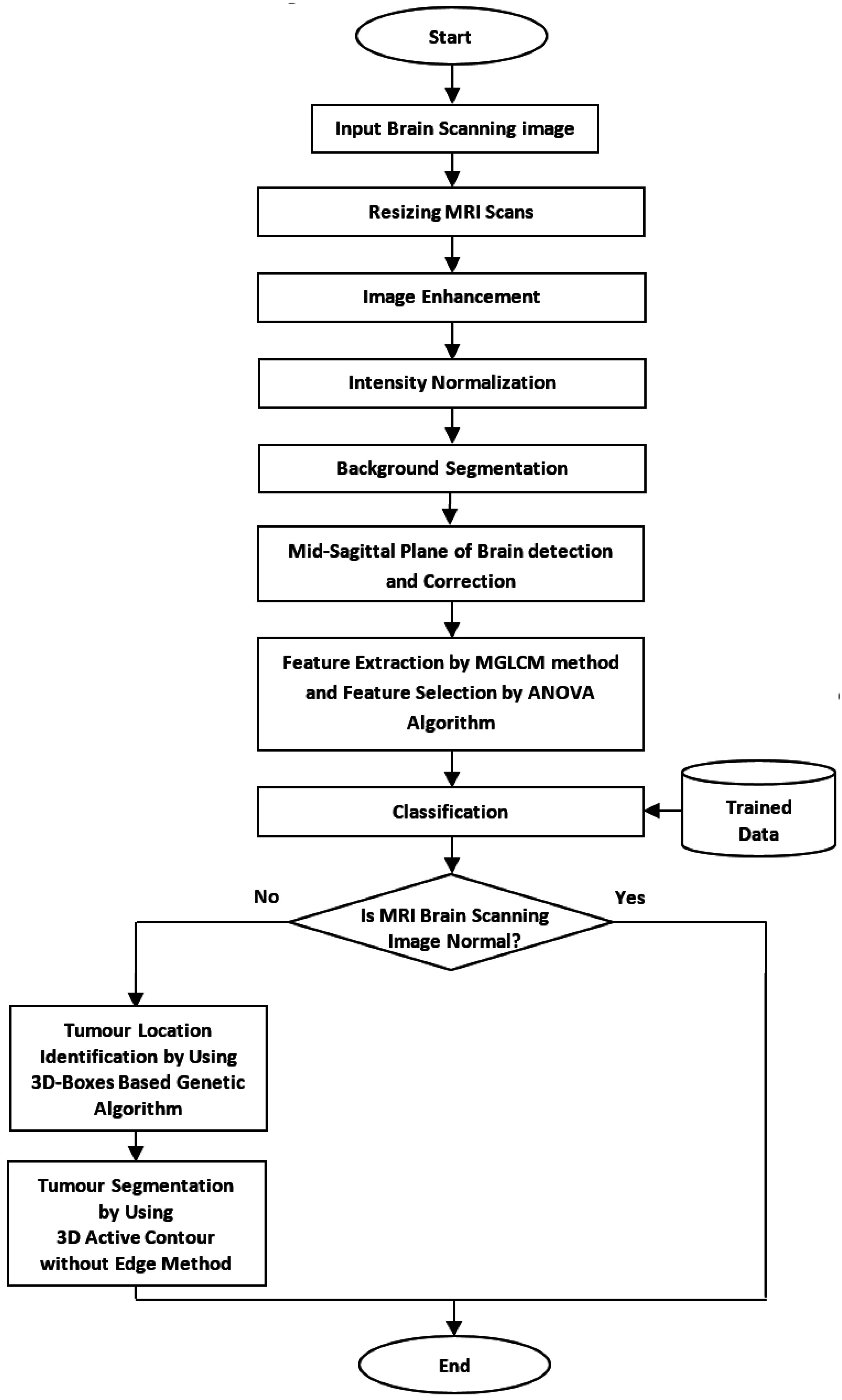
This research aimed to develop an automated method that can locate the initial contour of brain tumor segmentation across all axial slices of volumetric MRI brain scans. The overall flow chart of the proposed method is shown in Figure 1.

2.1. Data Collection

The clinical image dataset consists of 165 MRI brain scans acquired during routine diagnostic procedure at the MRI Unit in Al-Kadhimiya Teaching Hospital in Baghdad, Iraq. This dataset was diagnosed and classified into normal and abnormal by the clinicians of this unit. The MRI slice sets were obtained using a SIEMENS MAGNETOM Avanto 1.5 Tesla scanner (Malvern, PA, USA) and PHILIPS Achieva 1.5 Tesla scanner (Best, Netherlands). The provided dataset consisted of tumors with different sizes, shapes, locations, orientations, and types. A total of 88 patients in this dataset exhibited different brain abnormalities with tumor sizes, shapes, locations, orientations, and types. The remaining patient images exhibited no detectable pathology. The dataset included the four MRI image modalities, namely, T2-w, T1-w, T1c-w, and FLAIR images, under axial viewing and 3–5 mm slice thickness. An additional enhanced dataset of 50 pathological patients was prepared, although the brain tumors were manually segmented and labeled by an expert in this unit who evaluates segmentation algorithm accuracy.

The standard benchmark Multimodal Brain Tumor Segmentation dataset (BRATS 2013) obtained from the International Conference on Medical Image Computing and Computer-Assisted Interventions [8] was adopted to evaluate the proposed method.

2.2. Image Preprocessing

The preprocessing step involved the performance of a set of algorithms on MRI brain scan slices as a preparation for the feature extraction step. This step included dimension resizing of the MRI slices, image enhancement by Gaussian filter, and normalization of MRI image intensity because of image intensity variation. Finally, mid-sagittal plane (MSP) detection and correction algorithm were implemented.

2.2.1. Resizing the Dimensions of MRI (Magnetic Resonance Imaging) Slices

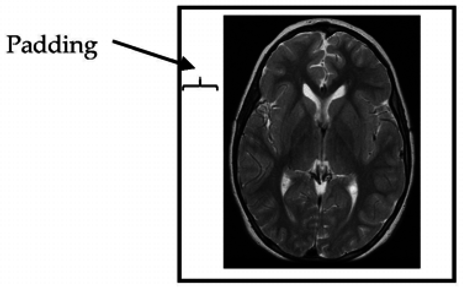
The provided MRI brain slices were collected from two scanners with different spatial resolutions. To enable the use of the full set without bias, the MRI scans were resized to 512 × 512 pixels. All algorithms developed in this study were implemented on squared slices. When the dimensions of the given MRI slices were changed to a square ratio, care was taken to maintain the ratio of voxels to pixels (e.g., pixel spacing). The MRI slices were then resized by adding additional columns from the left and right and additional rows from the top and bottom portions of the MRI slice until the slice size became 512 × 512 pixels in resolution (Figure 2).

2.2.2. MRI Enhancement Algorithm

The typical noise in MRI images appeared as a small random modification of the intensity in an individual or a small groups of pixels. These differences can be sufficiently large to lead to erroneous segmentation. A spatial domain low-pass filter (Gaussian filter, The Math Works, Natick, MA, USA) was used and contributed a negative effect to the responses of noise smoothing linear image enhancement. Consequently, the performance of the Gaussian filter was evaluated visually because of its preferably low value for σ [11,12].

2.2.3. Intensity Normalization

The pixel intensity values of each MRI slice were normalized to the same intensity interval to achieve dynamic range consistency. Histogram normalization was then applied to stretch and shift the original histogram of the image and cover all the grayscale levels in the image. The resulting normalized image achieved a higher contrast than that of the original image because the histogram normalization method enhanced image contrast and provided a wider range of intensity transformation. This approach demonstrated an enhanced classification of pathological tissues that can be achieved using the unmodified image [13].

2.2.4. Background Segmentation

Prior knowledge suggests that the background intensity values of MRI brain slices often approaches zero to enable background segmentation. The ability to eliminate and exclude the background from the region of interest is important because the background normally contains a much higher number of pixels than that of the brain region but without meaningful information [13]. In this study, histogram thresholding was used as a segmentation method to isolate the background. This approach is based on the thresholding of intensity values by a specific T value. Subsequently, the application employs a set of morphological operators to remove any hole appearing in the region. Notably, the T2-w MR image histograms attained almost identical distribution shapes [14]. Therefore, the T value was selected experimentally and set to 0.1 after the effects of a range of threshold values (0.05, 0.1, 0.2, and 0.3) were manually observed. Hence, if an intensity value of a pixel is less than 0.1, the pixel is considered as a background.

2.2.5. Mid-Sagittal Plane Detection and Correction

Mid-sagittal plane identification is an important initial step in brain image analysis because this method provides an initial estimation of the brain’s pathology assessment and tumor detection. The human brain is divided into two hemispheres with an approximately bilateral symmetry around the MSP. The two hemispheres are separated by the longitudinal fissure, which represents a membrane between the left and right hemisphere. MSP extraction methods can be divided into two groups as follows. Content-based methods find a plane that maximizes a symmetrical measure between both sides of the brain. By contrast, shape-based methods use the inter-hemispheric fissure as a simple landmark to extract and detect the MSP. In this study, we focused on determining the orientation of the patient’s head instead of measuring the symmetry to identify the brain MSP [3].

2.3. Feature Extraction

The fundamental objective of any diagnostic medical imaging investigation is tissue characterization. Texture analysis is commonly used to provide unique information on the intensity variation of spatially related pixels in medical images [2]. The choice of an appropriate technique for feature extraction depends on the particular image and application [4]. Texture features are extracted from MRI brain slices to encode clinically valuable information by using modified gray-level co-occurrence matrix (MGLCM). This method is a second-order statistical method proposed by Hasan and Meziane [3] to generate textural features and provide information about the patterning of MRI brain scan textures. These features are used to measure statistically the degree of symmetry between the two brain hemispheres. Symmetry is an important indicator that can be used to detect the normality and abnormality of the human brain. MGLCM generates texture features by computing the spatial relationship of the joint frequencies of all pairwise combinations of gray-level configuration of each pixel in the left hemisphere. These pixels are considered as reference pixels, with one of nine opposite pixels existing in the right hemisphere under nine offsets and one distance. Therefore, nine co-occurrence matrices are generated for each MRI brain scanning image.

To reduce the dimensionality of the feature space, we added the resultant MGLCM matrices of all the MRI slices at all orientations. The maximum number of gray levels considered for each image was typically scaled down to 256 gray levels (8 bits/pixel), rather than using the full dynamic range of 65,536 gray levels (16 bits/pixel) before computing the MGLCM. This quantization step was essential to reduce a large number of zero-valued entries in the co-occurrence matrix [15,16]. The computing time for implementing MGLCM for each slice was about 2.3 min by using an HP workstation Z820 (Natick, MA, USA) with Xeon E5-3.8 GHz (Quad-Core) and 16 GB of RAM (random access memory).

2.3.1. Feature Aggregation

The MGLCM method determines nine co-occurrence matrices. For each matrix, 21 statistical descriptors are determined, generating 189 descriptors for each MRI brain scan [3]. The cross correlation descriptor is also determined for the original MRI brain scan. Accordingly, 190 descriptors are attained for each MRI brain scan image. These features are used by the subsequent classification to differentiate between normal and abnormal brain images.

2.3.2. Feature Selection

High-dimensional feature sets can negatively affect the classification results because high numbers of features may reduce the classification accuracy owing to the redundancy or irrelevance of some features. Feature-selection techniques aim to identify a small subset of features that minimizes redundancy and maximizes relevancy. Therefore, feature selection is an important step in exposing the most informative features and for optimally tuning the classifier’s performance to reliably classify unknown data. In this study, ANOVA was employed to measure feature significance and relevance [3].

2.4. Classification

Classification is the process of sorting objects in images into separate classes and plays an important role in medical imaging, especially in tumor detection and classification. This step is also a common process employed in many other applications, such as robotic and speech recognition [4]. In the present study, a multi-layer perceptron neural network (MLP) was adopted to classify MRI brain scans into normal and abnormal images. MLP is used in different applications, such as optimization, classification, and feature extraction [3].

2.5. Brain Tumors Location Identification

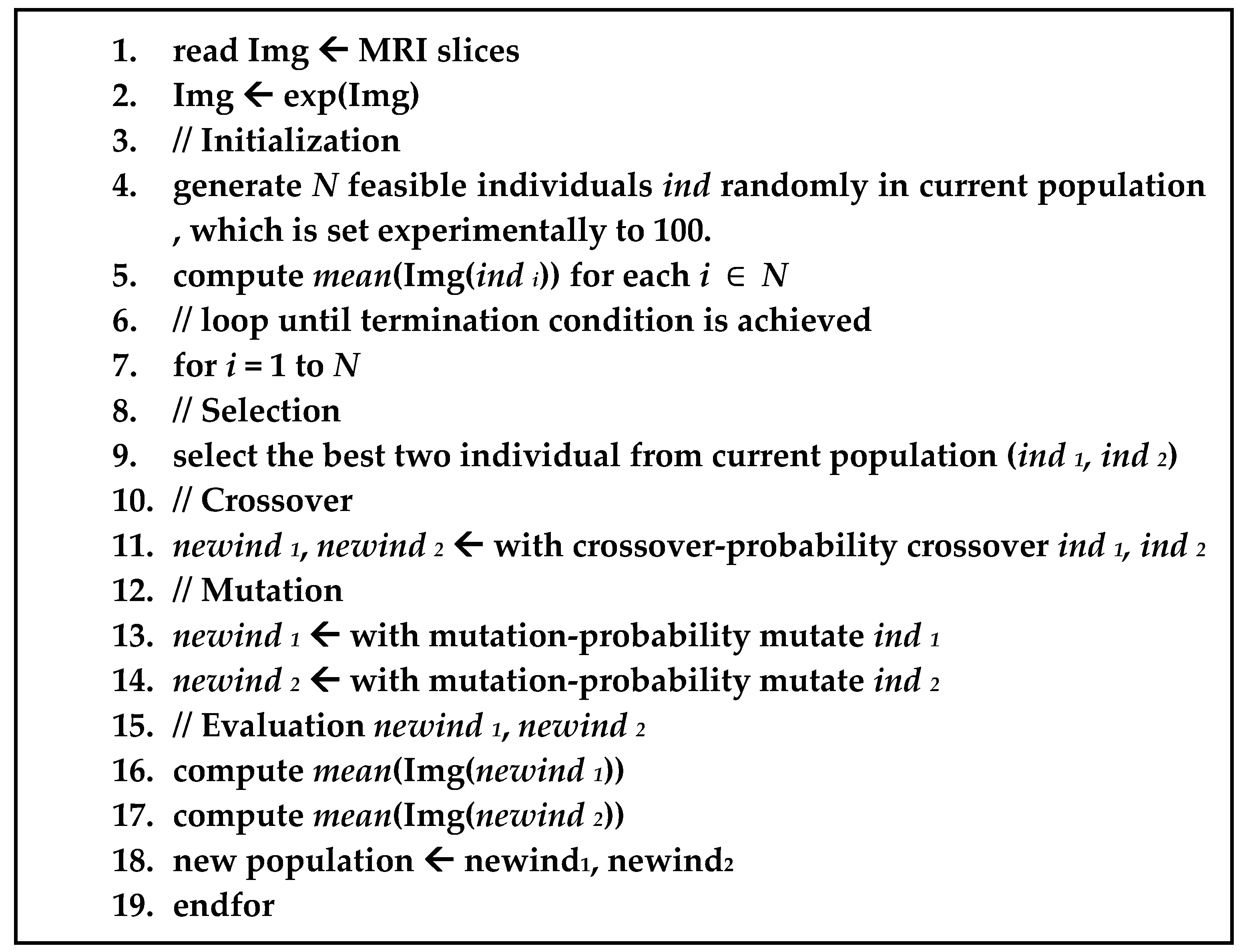
Many tumor-segmentation methods are not fully automated. These approaches require user involvement in selecting a seed point. Usually, the MRI slices of a patient are interpreted visually and subjectively by radiologists, in which tumors are segmented by hand or by semi-automatic tools. Both manual and semiautomatic approaches are considered as tedious, time-consuming, error-prone processes. Tumors are more condensed than the surrounding material and present as brighter pixels than the surrounding brain tissue. Therefore, the basic concept of brain tumor detection algorithms is finding pixel clusters with a different or higher intensity than that of their surroundings. In this study, a bounding 3D-box-based genetic algorithm (BBBGA) method was proposed by Hasan [17] to search and identify the location of most dissimilar regions between the left and right hemispheres of the brain automatically without the need for user interaction. The input was a set of MR slices belonging to the scans of a single patient, and its output was a subset of slices covering and circumscribing the tumor with a 3D box. The BBBGA method exploits the symmetry feature of axial viewing of MRI brain slices to search for the most dissimilar region between the left and right brain hemispheres. This dissimilarity is detected using genetic algorithm (GA) and an objective-function-based mean intensity computation. The process involves randomly generating hundreds of 3D boxes with different sizes and locations in the left brain hemisphere. Such boxes are then compared with the corresponding 3D boxes in the right brain hemisphere through the objective function. These 3D boxes are moved and updated during the iterations of the GA toward the region that maximized the objective function value. An advantage of the BBBGA method is its lack of necessity for image registration or intensity standardization in MR slices. The approach is an unsupervised method; hence, the problems on observer variability in supervised techniques are ignored.

Prior to BBBGA, exponential transformation is implemented to compress the low-contrast regions in MRI brain images and expand the high-contrast regions in a nonlinear manner. This action would increase the intensity difference between the brain tumor and the surrounding soft tissue [17,18]. Figure 3 illustrates the pseudo-code for BBBGA.

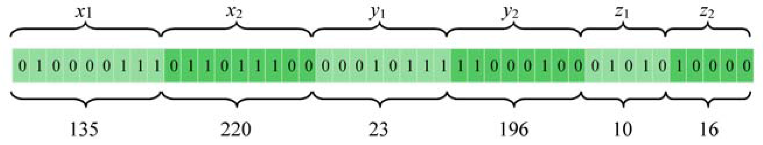
For additional details on how each individual in the GA population is mapped into binary form, we use the following scenario. Suppose we have a MRI brain scan (dimensions 512 × 512 × 32 pixels) of a pathological patient, each individual in the GA population is denoted by the binary representation of the coordinates of one 3D box (x₁, x₂, y₁, y₂, z₁, and z₂). In this case, x₁ and x₂ represent the height of the 3D box and are subject to the constraints 1 ≤ x₁ < 512 and x₁ < x₂ ≤ 512. Meanwhile, y₁ and y₂ signify the width of the 3D box and are subject to the constraints 1 ≤ y₁ < 256 and y₁ < y₂ ≤ 256. Finally, z₁ and z₂ represent the depth of the 3D box and are subject to the constraints 1 ≤ z₁ < 32 and z₁ < z₂ ≤ 32. Herein, we assume that the maximum number of MRI slices is 32. Figure 4 shows an example of how the coordinates of 3D box (x₁, x₂, y₁, y₂, z₁, z₂) are mapped to the individual of GA in a binary form.

2.6. Three-Dimensional Brain Tumors Segmentation

The principal goal of the segmentation process is partitioning an image into meaningful and homogeneous regions with respect to one or more characteristics [4]. Subdivision levels of segmentation depend on the problem being solved. Segmentation in medical imaging is normally used to classify pixels to different anatomical regions, such as bones, muscles, and blood vessels. Furthermore, this function is used to classify the pixels of pathological regions, such as malignancies and necrotic and fibrotic areas.

Brain tumor segmentation is difficult to achieve using conventional methods (e.g., pixel-based, region-based, and edge-based methods) [10,19]. Additionally, given the appearance of volumetric 3D medical imaging data, the segmentation of these data for extracting boundary elements belonging to the same structure offers an additional challenge. Therefore, the deformable model was proposed to improve this concern by combining constraints derived from the image and a priori knowledge of the object, such as location, shape, and orientation. The deformable model was originally developed to solve a set of problems in computer vision and medical image analysis. Both 2D and 3D deformable model variants have been applied to segment, visualize, track, and quantify various anatomic structures, such as brain tumors, heart, face, cerebral, coronary and retinal arteries, kidney, and lungs.

2.6.1. Level Set Method

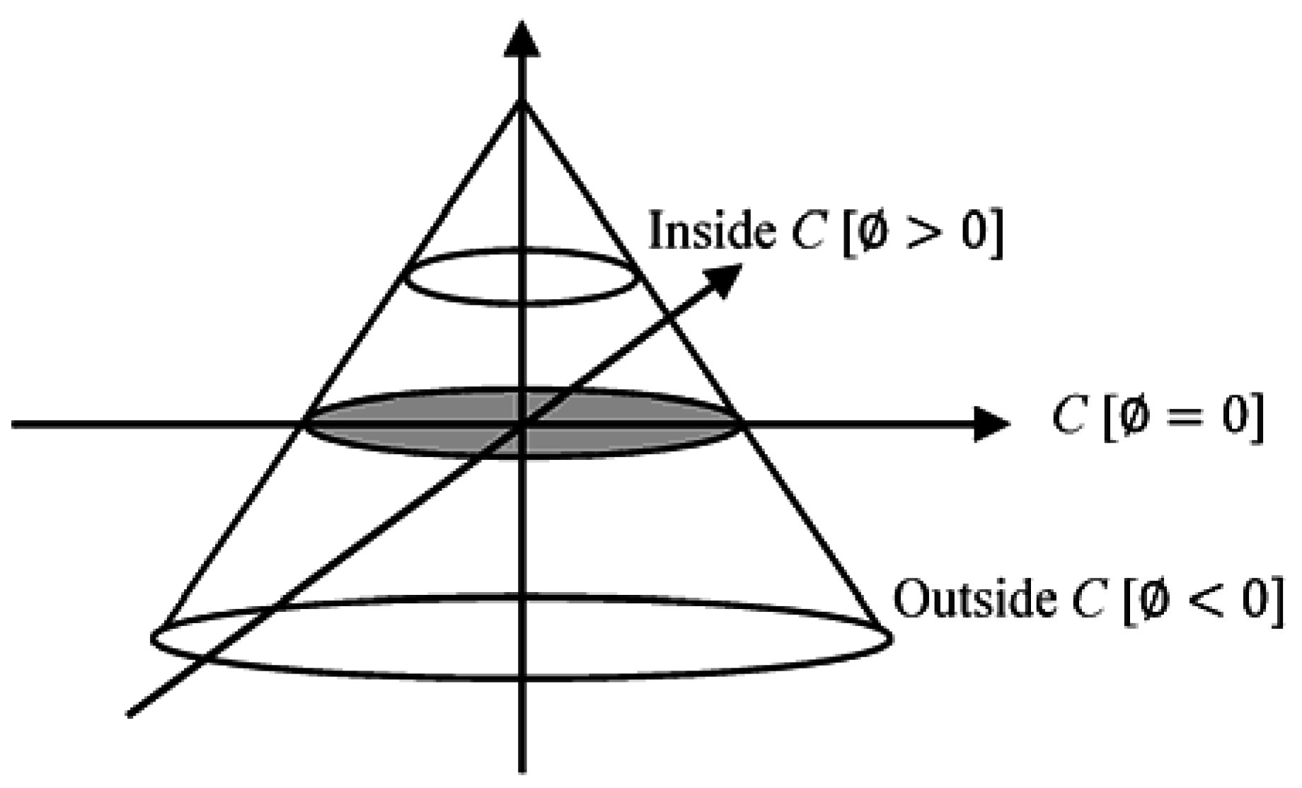
The level set method is a powerful tool for implementing contour evolution and managing topology changes. This approach simply defines an evolving contour C implicitly. This contour is represented by the zero-level set of a Lipschitz continuous function as given in Equation (1):

$$\varnothing :\mathsf{\Omega }\to ℝ$$

where

$$\begin{array}{c}C=\left[\left(x,y\right)\in \mathsf{\Omega };\varnothing \left(x,y\right)=0\right]\\ C_{inside}=\left[\left(x,y\right)\in \mathsf{\Omega };\varnothing \left(x,y\right)>0\right]\\ C_{outside}=\left[\left(x,y\right)\in \mathsf{\Omega };\varnothing \left(x,y\right)<0\right]\end{array}$$

(1)

where x and y are coordinates in the image plane. The level set function simultaneously defines both an edge contour and a segmentation of the image.

A crucial step is determining the set function level that segments the image to different important regions. This step is achieved by defining the level set function through subtracting the threshold from each pixel gray-level value. This action results in a level set function positive in regions where the gray level exceeds the threshold (Figure 5) [20].

2.6.2. 3DACWE (Three-Dimensional Active Contour without Edge)

The 3DACWE method, also known as Chan–Vese model, is an example of a geometrically active contour model [21]. The initial contour is evolved using a level set method and does not rely on the gradient of the image for the stopping process. The stopping process of the contour is based on minimizing the Mumford–Shah function [20,21]. Therefore, the 3DACWE method can detect object boundaries not necessarily defined by the gradient, even if the object boundaries are highly smooth or discontinuous.

The 3DACWE algorithm evolves the 3D level set function and minimizes the Mumford–Shah function by setting the value of piecewise smooth function u. Moreover, the function u approximates the original image I besides smoothing the connected components in the image domain $\mathsf{\Omega }$.

Mumford and Shah proposed the energy function given in Equation (2), which can be used for segmenting an image I into non-overlapping regions [21,22,23,24]:

$${ℱ}^{MS}\left(u,C\right)=\underset{\mathsf{\Omega }}{\overset{}{{\displaystyle \int }}}{\left(u-I\right)}^{2}dxdydz+\mathsf{\mu }{{\displaystyle \int }}_{\mathsf{\Omega }/C}{\left|\nabla u\right|}^{2}dxdydz+v\left|C\right|$$

(2)

where the first term encourages u to be close to I, the second term ensures that u is differentiable on Ω/C, and the third term ensures regularity on C. To overcome the time complexity of solving the general Mumford and Shah function, it is required to suppose u to be constant on each connected component . An active contour approach was proposed by Chan and Vese [21] based on minimizing Mumford and Shah functional by penalizing the enclosed area assuming that u is supposed to have only the two values which are given in Equation (3) [24]:

$$u\left(x,y\right)=\{\begin{array}{c}{c}_{1}wherex,y,zareinsideC\\ c_{2}wherex,y,zareoutsideC\end{array}$$

(3)

where C is the boundary of a contour, and $c_1\mathrm{and}{c}_2$ are the values of u inside and outside the contour, respectively. The Chan–Vese energy function is given by Equation (4) [21,22,24]:

$${ℱ}^{CV}\left(C,c_1,c_2\right)=\mathsf{\mu }Length\left(C\right)+vArea\left(inside\left(C\right)\right)+{\mathsf{\lambda }}_1{{\displaystyle \int }}_{inside\left(C\right)}{\left|I\left(x,y,z\right)-c_1\right|}^{2}dxdydz+{\mathsf{\lambda }}_2{{\displaystyle \int }}_{outside\left(C\right)}{\left|I\left(x,y,z\right)-c_2\right|}^{2}dxdydz$$

(4)

The regularity is controlled by penalizing the length in the first term, and the size is controlled by penalizing the enclosed area of C.

These terms are called regularizing terms and are given in Equations (5) and (6), and encourage the contour C to be smooth and short, and can be written by using 3D-level set form $\varnothing$ as [21,25]

$$length\left(\varnothing \left(x,y,z\right)\right)={\int }_{\mathsf{\Omega }}{\delta }_o\left(\varnothing \left(x,y,z\right)\right)\left|\nabla \varnothing \left(x,y,z\right)\right|dxdydz$$

(5)

$$area\left(\varnothing \left(x,y,z\right)\right)={{\displaystyle \int }}_{\mathsf{\Omega }}H\left(\varnothing \left(x,y,z\right)\right)dxdydz$$

(6)

${\lambda }_1,{\lambda }_2,$ $\mathsf{\mu }\ge 0,$ and $v\ge 0$ are fixed parameters controlling selectivity, where the energy function is minimized by fixing these parameters optimally. Meanwhile, ${\mathsf{\lambda }}_1,{\mathsf{\lambda }}_2$ control the internal and external forces, respectively. These terms usually hold the same constant and hence cause a fair competition between these two regions [24]. Generally, ${\mathsf{\lambda }}_1={\mathsf{\lambda }}_2=1$ [21,26]. Meanwhile, $\mathsf{\mu }$ controls the smoothness of contour C and assumes a scaling role. However, the parameter is not constant across all experiments. If $\mathsf{\mu }$ is large, only larger objects with smooth boundaries are segmented. If $\mathsf{\mu }$ is small, objects of smaller size are segmented accurately [21,23,27]. Typically, $\mathsf{\mu }$ depends on image resolution, where $\mathsf{\mu }=0.1\times {255}^2$ [26]. Meanwhile, v sets the penalty for the area inside the contour C. This parameter is essential only when two sides of boundaries (internal and external boundaries) are present in the desired object [23]. ${\mathsf{\delta }}_o$ is a 2D Dirac function that represents $\frac{d}{d\varnothing }H\left(\varnothing \left(x,y\right)\right)$. $\nabla$ (Equation (5)) is the gradient operator, and H is the Heaviside function [20,21,22,25]. Accordingly, by using the 3D-level set function, we can rewrite the Chan–Vese energy function in Equation (7) [28] as follows:

$${ℱ}^{CV}\left(\varnothing \left(x,y,z\right)\right)=\mathsf{\mu }{\int }_{\mathsf{\Omega }}{\mathsf{\delta }}_o\left(\varnothing \left(x,y,z\right)\right)\left|\nabla \varnothing \left(x,y,z\right)\right|dxdydz+v{\int }_{\mathsf{\Omega }}H\left(\varnothing \left(x,y,z\right)\right)dxdydz+{\mathsf{\lambda }}_1{\int }_{inside\left(C\right)}{\left|I\left(x,y,z\right)-c_1\right|}^{2}H(\varnothing \left(x,y,z\right)dxdydz+{\mathsf{\lambda }}_2{\int }_{outside\left(C\right)}{\left|I\left(x,y,z\right)-c_2\right|}^2(1-H\left(\varnothing \left(x,y,z\right)\right)dxdydz$$

(7)

The minimization is solved by alternatively updating $c_1,c_2$, and $\varnothing$, keeping $\varnothing$ fixed, and minimizing the energy function ${ℱ}^{CV}$ with respect to the optimal values $c_1$ and $c_2$. Consequently, Equations (8) and (9) are attained for $c_1$ and $c_2$ as functions of $\varnothing$:

$$c_1\left(\varnothing \left(x,y,z\right)\right)=\frac{{\int }_{\mathsf{\Omega }}^{}I\left(x,y,z\right).H\left(\varnothing \left(x,y,z\right)\right)dxdydz}{{\int }_{\mathsf{\Omega }}^{}H\left(\varnothing \left(x,y,z\right)\right)dxdydz}$$

(8)

$$c_2\left(\varnothing \left(x,y,z\right)\right)=\frac{{\int }_{\mathsf{\Omega }}^{}I\left(x,y,z\right).\left(1-H\left(\varnothing \left(x,y,z\right)\right)\right)dxdydz}{{\int }_{\mathsf{\Omega }}^{}\left(1-H\left(\varnothing \left(x,y,z\right)\right)\right)dxdydz}$$

(9)

To minimize the energy function ${ℱ}^{CV}$ with respect to $\varnothing$ and fix the $c_1$ and $c_2$, a gradient descent method is adopted and has yielded the associated Euler-Lagrange equation for $\varnothing$, which is given by Equation (10) (parameterizing the descent direction by an artificial time) [21,22,27,29,30]:

$$\{\begin{array}{c}\frac{\partial \varnothing }{\partial t}=\mathsf{\delta }(\varnothing )\left[\mathsf{\mu }div\left(\frac{\nabla \varnothing }{\left|\nabla \varnothing \right|}\right)-v-{\mathsf{\lambda }}_1{\left(I\left(x,y\right)-c_1\right)}^2+{\mathsf{\lambda }}_2{\left(I\left(x,y\right)-c_2\right)}^2\right]in\mathsf{\Omega }\\ \frac{\mathsf{\delta }(\varnothing )}{\left|\nabla \varnothing \right|}\frac{\partial \varnothing }{\partial \overrightarrow{n}}=0on\partial \end{array}$$

(10)

where, $\overrightarrow{n}$ represents the exterior normal to the boundary of ∂Ω, and $\frac{\partial \varnothing }{\partial \overrightarrow{n}}$ represents the normal derivative of $\varnothing$ at the boundary.

2.6.3. Evaluation of the Segmentation

Image segmentation evaluation can be categorized into subjective and objective evaluation. The subjective evaluation method requires to compare visually the result of the image [31]. While the objective evaluation is divided into supervised and unsupervised techniques. Supervised evaluation methods evaluate segmentation algorithms by comparing segmentation results with manually-segmented reference images which are segmented by experts. It is also known as ground truth reference images or gold standard. While unsupervised evaluation methods do not require to compare with any additional reference images but it just relies on the degree of matching among the characteristics of segmented images as desired by humans. The main advantage of unsupervised evaluation method is that it does not need to compare against a manual segmented reference image. This merit makes it more suitable for real-time application where a large number of images with unknown content and no ground truth need.

In this study supervised evaluation is preferred because of the complexity of the brain tissue and variety of brain tumors. It measures the degree of similarity between the segmented MRI brain tumors and those that are segmented manually or with ground truth dataset. A set of statistical measures have been used to evaluate the segmentation outcomes. They are True Positive (TP), False Positive (FP), True Negative (TN), and False Negative (FN). Such that the TP denotes number of pixels that are correctly segmented as part of a tumor, FP denotes number of pixels that are incorrectly segmented as part of a tumor, FN denotes number of pixels that are incorrectly segmented as healthy pixels, and TN denotes number of pixels that are correctly segmented as healthy pixels. These measures are used to evaluate the segmentation process; accuracy, sensitivity, and specificity. Accuracy is defined as the ratio of numbers of pixels that are correctly segmented to the total number of pixels in MRI slices (Equation (11)). Sensitivity considers the proportion of the tumor that is correctly segmented (Equation (12)). Specificity refers to the proportion of the non-tumor region that is correctly segmented and is given in Equation (13) [8].

$$Accuracy=\frac{\mathrm{TP}+\mathrm{TN}}{\mathrm{TP}+\mathrm{TN}+\mathrm{FP}+\mathrm{FN}}\times 100\%$$

(11)

$$Sensitivity=\frac{\mathrm{TP}}{\mathrm{TP}+\mathrm{FN}}\times 100\%$$

(12)

$$Specificity=\frac{\mathrm{TN}}{\mathrm{TN}+\mathrm{FP}}\times 100\%$$

(13)

In the evaluation of segmentation, both accuracy and specificity are not highly relevant because these two measures adopt the TN, which depends on the relative size of the MRI image and the object of interest. Therefore, the following additional metrics are used to evaluate the segmentation results: Dice, Jaccard, and matching coefficients [32,33].

3. Experimental Results

Experiments were performed using MATLAB R2015a (The Math Works, Natick, MA, USA), on Windows 10. The collected dataset is initially classified into normal and pathological cases to train the algorithms and evaluate the classification and tumor identification accuracy by cross-validation. The standard (BRATS 2013) dataset is then used to evaluate the accuracy of the proposed 3D segmentation system.

3.1. Classification Results

For each MRI image, 190 features were extracted using the MGLCM method. The highest classification accuracy with the optimum performance was achieved by the MLP network at 91% accuracy for correctly classifying the collected dataset by cross validation.

In this study, ANOVA was used for relevance analysis. The critical value α was set to 0.001 to obtain highly significant features [34]. The assessment of predictors depends on both F-statistic value and p-value because a p-value less than 0.001 is insufficient for a predictor. Instead, the predictor must also hold a high F-statistic value. The high F-statistic value indicates that the classes significantly separated from one another [17]. The differences between the features of normal and abnormal MRI brain scan groups of the co-occurrence matrix at θ₁ = 0 and θ₂ = 0 is shown in

Table 1. Comparison of MRI brain scan features (mean ± standard deviation (SD)) between normal and abnormal patients.

Features	Abnormal MRI Scans	Normal MRI Scans	F-Statistic	p-Value
Auto correlation (×103)	5.62 ± 1.2	4.92 ± 1.24	13.67	<0.001
Contrast (×103)	1.89 ± 0.618	0.918 ± 0.22	166.2	<0.001
Correlation (÷10)	7.1 ± 0.91	8.07 ± 0.72	291.5	<0.001
Cluster Prominence (×108)	3.6 ± 1.87	2.7 ± 1.09	14.62	<0.001
Cluster Shade (×105)	7.6 ± 4.26	5.5 ± 2.9	13.14	<0.001
Dissimilarity (×10)	2.42 ± 0.47	1.58 ± 0.21	209	<0.001
Energy (÷10)	1.02 ± 0.2	1.05 ± 0.18	368.15	<0.001
Entropy	7.07 ± 0.336	6.87 ± 0.25	15.21	<0.001
Homogeneity (÷10)	3.55 ± 0.34	3.76 ± 0.26	451.3	<0.001
Max. Probability (÷10)	3.17 ± 0.33	3.23 ± 0.28	444.96	<0.001
Sum of Square Variance (×103)	6.5 ± 1.6	5.38 ± 1.23	24.36	<0.001
Sum Average (×102)	1.15 ± 0.112	1.06 ± 0.15	20.84	<0.001
Sum Variance (×104)	2.33 ± 0.47	1.97 ± 0.48	24.25	<0.001
Sum Entropy	4.46 ± 0.177	4.16 ± 0.147	35.98	<0.001
Difference Entropy	3.64 ± 0.2	3.34 ± 0.124	132.2	<0.001
Information Measure of Correlation I (÷10)	−2.24 ± 0.3	−2.53 ± 0.26	430.15	<0.001
Information Measure of Correlation II (÷10)	9.11 ± 0.2	9.26 ± 0.18	355.48	<0.001
Inverse difference Normalized (÷10)	9.25 ± 0.12	9.48 ± 0.06	407.8	<0.001
Inverse difference Moment Normalized (÷10)	9.78 ± 0.07	9.87 ± 0.028	316.89	<0.001
Weighted Mean (÷10)	−8.73 ± 84	0.53 ± 18.7	0.92	0.339
Weighted Distance	3.05 ± 2.91	0.77 ± 0.52	46.1	<0.001
Cross Correlation (÷10)	7.1 ± 0.91	8.07 ± 0.72	291.5	<0.001

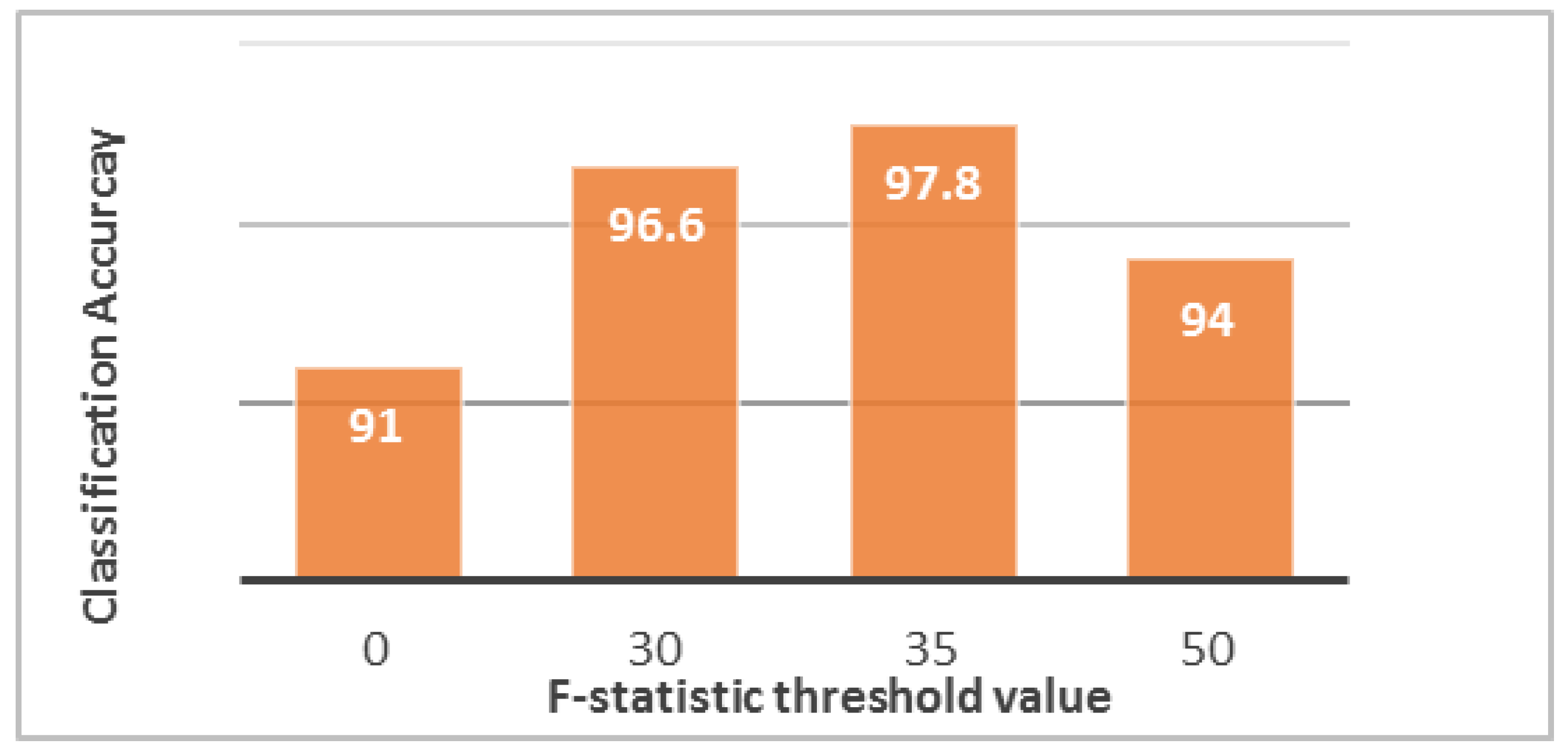
. All features seemed acceptable except the weighted mean predictor. Nevertheless, significant variation existed in the F-statistic values between features, indicating a degree of significant difference between the selected features. The p-value does not actually signify the degree of separation of each group from others and ignores feature redundancy [35]. This drawback is overcome by the F-statistic to determine the power of feature discrimination through thresholding, in which different threshold values are taken to ignore the redundant features and evaluate the selected features at each time by observing the performance of the classifier. When the F-statistic threshold value increases, the numbers of selected predictors and the vector of the features decrease. The optimal threshold value that can provide the highest accuracy is 35 (Figure 6). Under this condition, only one normal patient was classified incorrectly as pathological, and three pathological patients were classified incorrectly as normal. Thus, some patients may be misclassified in both ways, but the high classification accuracy (97.8%) reduces these cases to a very small number. These cases are not treated and are passed to the segmentation phase as “erroneous cases.”

Consequently, 11 relevant and significant features for each angle of the MGLCM are selected by ANOVA, namely, contrast, correlation, dissimilarity, sum of square variance, sum average, sum variance, difference entropy, information measure of correlation I, inverse difference normalized (IDN), inverse difference moment normalized, and weighted distance, in addition to the cross correlation.

3.2. Tumor Identification Results

The main factor that differentiates tumor from healthy tissue is tumor brightness relative to the surrounding brain tissue. Therefore, brain tumor detection algorithms are based mainly on finding pixel clusters with a different intensity from that of their surroundings on the basis of brain symmetry.

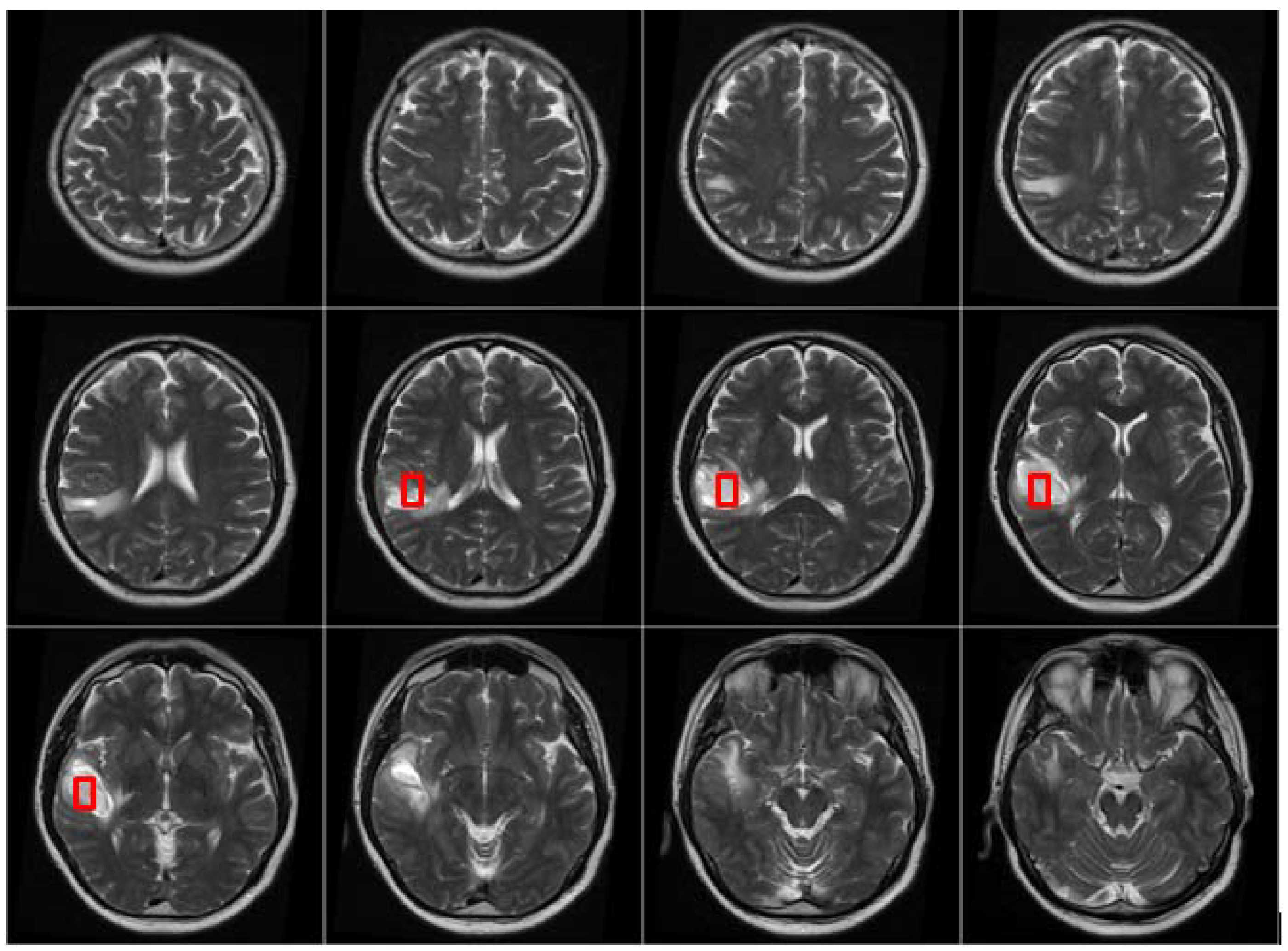
After the MRI brain scans are classified into normal and pathological images, the BBBGA method was applied on those identified as pathological cases as shown in the pathological patient in Figure 7. The red rectangles denoting the optimized 3D box refer to the pathological area in slices 6–9 where the tumor appears.

The BBBGA method was implemented on MRI brain slices of pathological patients with population size (N) equal to 100. The individuals were selected using the roulette wheel selection method because this approach is more popular and efficient in different applications [36]. The selected individuals were then mated using a multi-point crossover with probability of 0.5 [37]. Finally, a single-point mutation was implemented with a probability of 0.05.

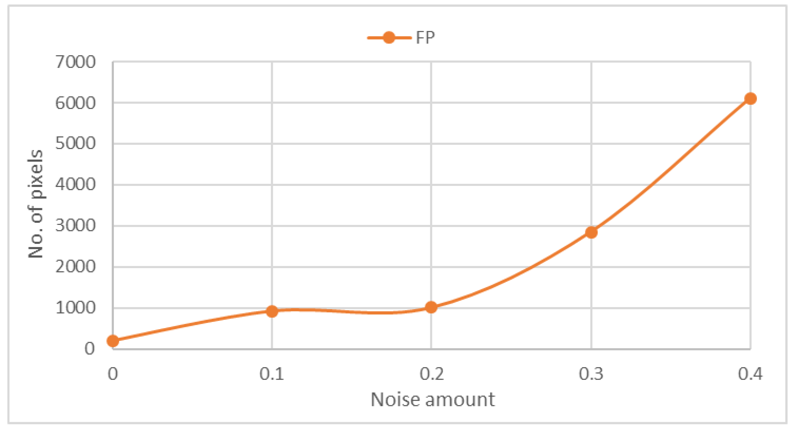
Evidence extracted from previous studies [18,38] indicates the lack of a standard method for evaluating the BBBGA approach. Saha, et al. [38] used an example to observe and measure the noise sensitivity of this approach by adding Gaussian noise with different amounts of $\mathsf{\sigma }=$ 0, 0.1, 0.2, 0.3, and 0.4 although this addition is not important and irrelevant to evaluation. We measure the noise sensitivity of our approach after the addition of Gaussian noise of the same noise amounts. Figure 8 shows that FP is proportional to the amount of noise in the MRI scan. Hence, our approach was evaluated using the collected dataset that included 88 pathological cases. Among 84 pathological cases, an abnormality was successfully located. Only four cases remained undetected because of the method’s inability to detect hardly visible tumors of size less than 1 cm³. Moreover, tiny tumors hold a spatial scale relatively similar to normal anatomic variability [39].

3.3. Tumor Segmentation Results

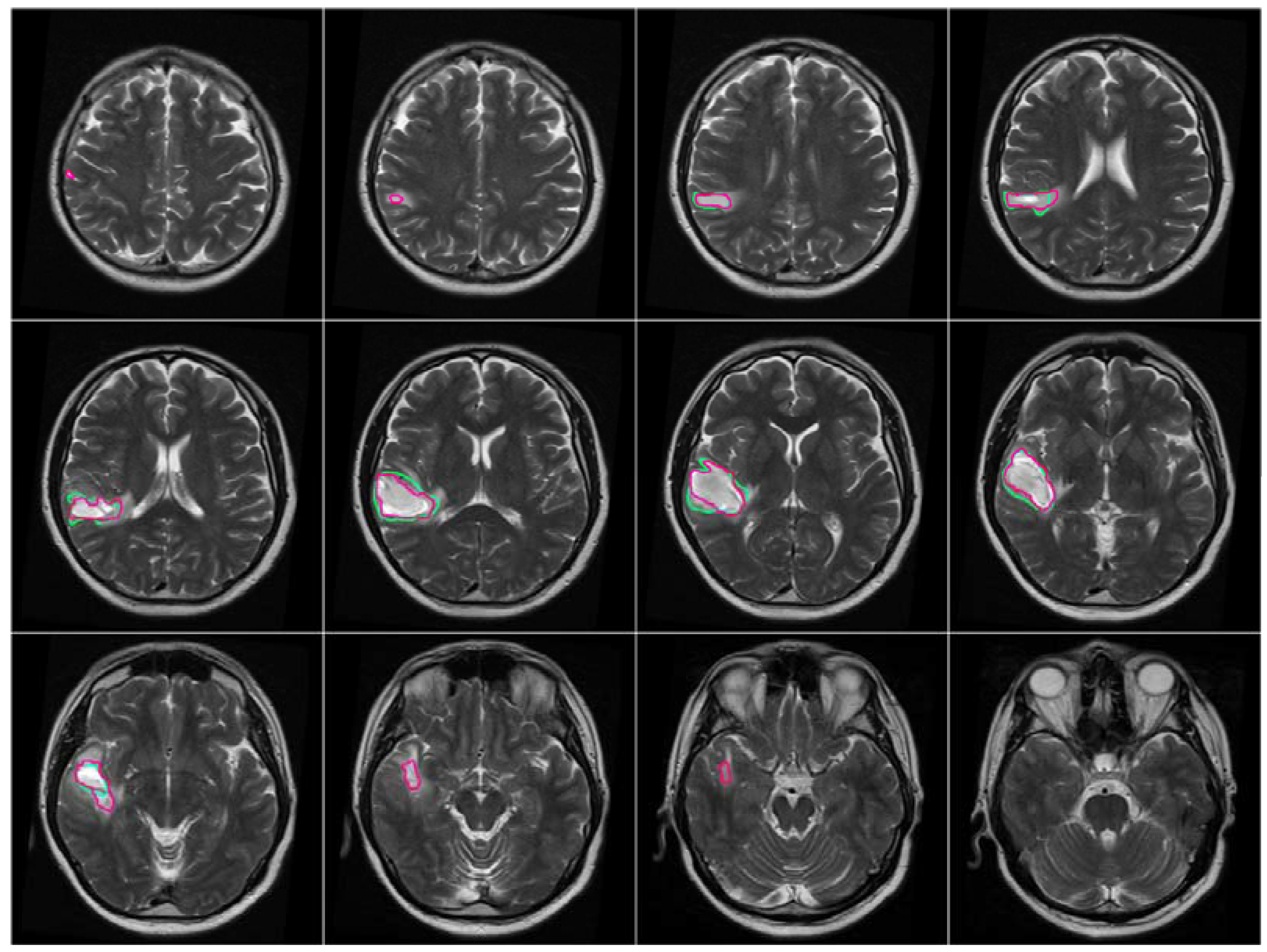
After the brain tumor location was recognized and identified by BBBDG, the 3DACWE approach was initialized and applied to the T2-w MRI brain scan images of 12 MRI slices from the collected dataset (Figure 9). The ground truth provided by the clinician are marked in green, and the tumor boundaries extracted by 3DACWE are marked in red. This patient holds a brain tumor in the left brain hemisphere. The 3DACWE was initialized by the following initial parameters: λ₁ = λ₂ = 1 and length penalty μ = 106.

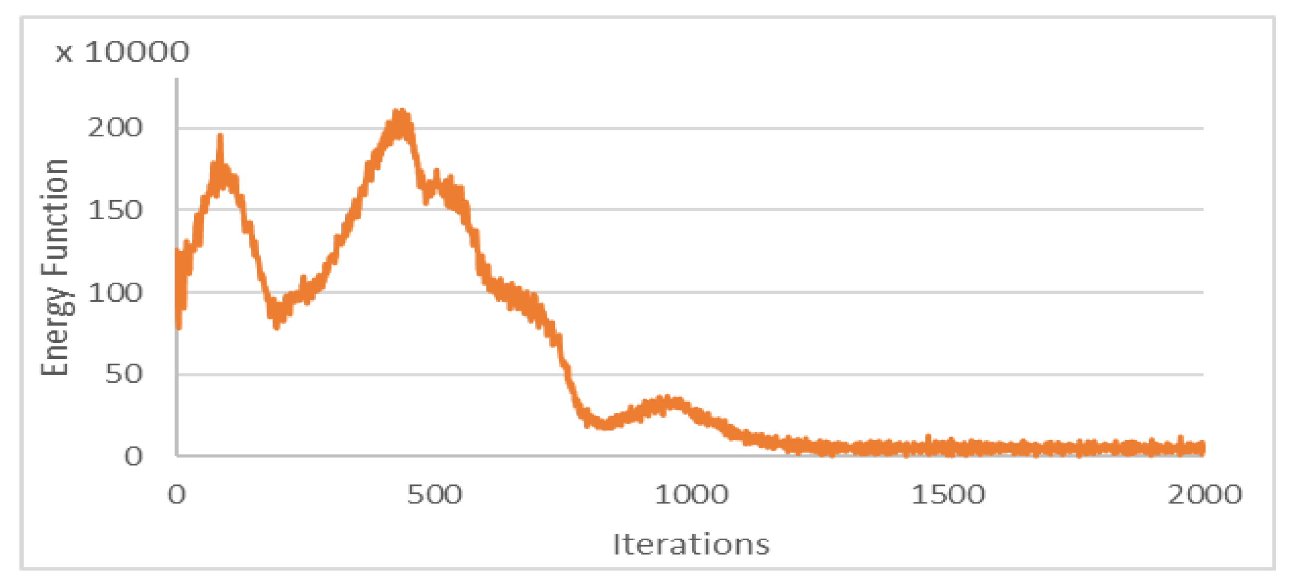
The Chan–Vese energy function was minimized within the iterations of 3DACWE and reached a steady state in 1250 iterations (Figure 10). This patient’s MRI scan was segmented with a Dice score of 88.4% by comparing with manual segmentation.

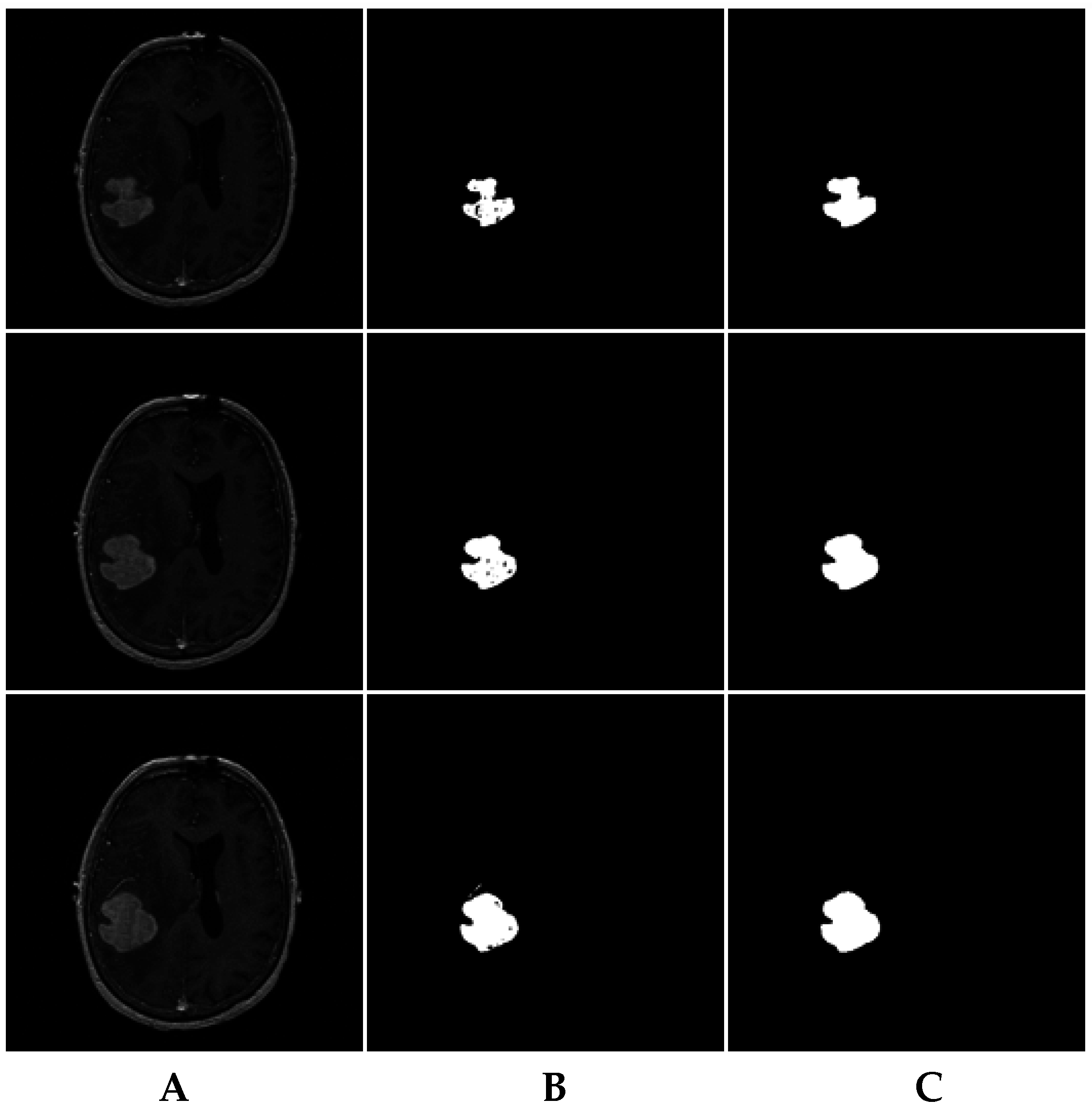
Under this segmentation process, some brain tumor parts in the MRI slices were incorrectly segmented as healthy tissues, and some healthy brain tissues were incorrectly segmented as pathological tissues. To eliminate these ambiguities and reduce the FPs and FNs, a consistency verification algorithm was applied for post-processing [11,40]. The majority filter was adopted to remove the FPs and FNs by replacing the segmented pixels inconsistent with their neighboring segmented pixels in a certain neighborhood. For example, if the center pixel of a window is segmented as a tumor but the majority of the neighboring pixels were segmented as healthy, then the center pixel is changed to healthy. Otherwise, if a pixel within the tumor area is segmented incorrectly as healthy and is surrounded by pixels that are segmented as tumor, then the pixel is changed to a pathological pixel. If the window size of the applied filter is increased, the quality of the output image significantly augments at the expense of complexity increase [40]. Herein, consistency verification was applied in a 5 × 5 neighborhood window [11].

For instance, the MRI brain slices in Figure 11A include some MRI slices with incorrectly segmented pixels (Figure 11B). The consistency verification algorithm results are shown in Figure 11C.

Table 2. Segmentation results for each patient in the collected dataset.

Results	Sensitivity	Specificity	Accuracy	Dice Index	Jaccard	Matching
Average	0.854	0.999	0.998	0.890	0.804	0.854
STD	0.069	0.001	0.002	0.047	0.075	0.069
Min	0.690	0.996	0.994	0.764	0.619	0.690
Max	0.971	1.000	1.000	0.956	0.915	0.971

and

Table 3. Segmentation results for each patient in the BRATS 2013 dataset.

Results	Sensitivity	Specificity	Accuracy	Dice Index	Jaccard	Matching
Average	0.909	1.000	0.999	0.893	0.809	0.909
STD	0.076	0.000	0.000	0.043	0.068	0.076
Min	0.736	0.998	0.998	0.768	0.624	0.736
Max	0.999	1.000	1.000	0.947	0.899	0.999

demonstrate the average results of segmentation for both collected and BRATS 2013 datasets, respectively, in which the collected dataset was manually segmented by experts.

The overall results of the segmentation of the four MRI modalities (T1-w, T2-w, T1c-w, and FLAIR) for the collected dataset with the four most common metrics reported in previous studies (accuracy, Dice, Jaccard, and matching methods) are summarized in Figure 12. The T1c-w-based segmentation attained the highest average metric rates because of contrast enhancement of the pathological tissues. The T2-w-based segmentation was rated as the lowest among all metrics because of highly inhomogeneous intensity distribution despite the sharp edges and high intensity of brain tumor with respect to the surrounding tissues.

Table 4. Comparison of tumor segmentation accuracy (mean ± SD) using 2DACWE and 3DACWE.

Method	T2-w	T1-w	T1c-w	FLAIR
2DACWE	83.73% ± 4.6%	84.43% ± 5.3%	86.6% ± 3.4%	82% ± 4.5%
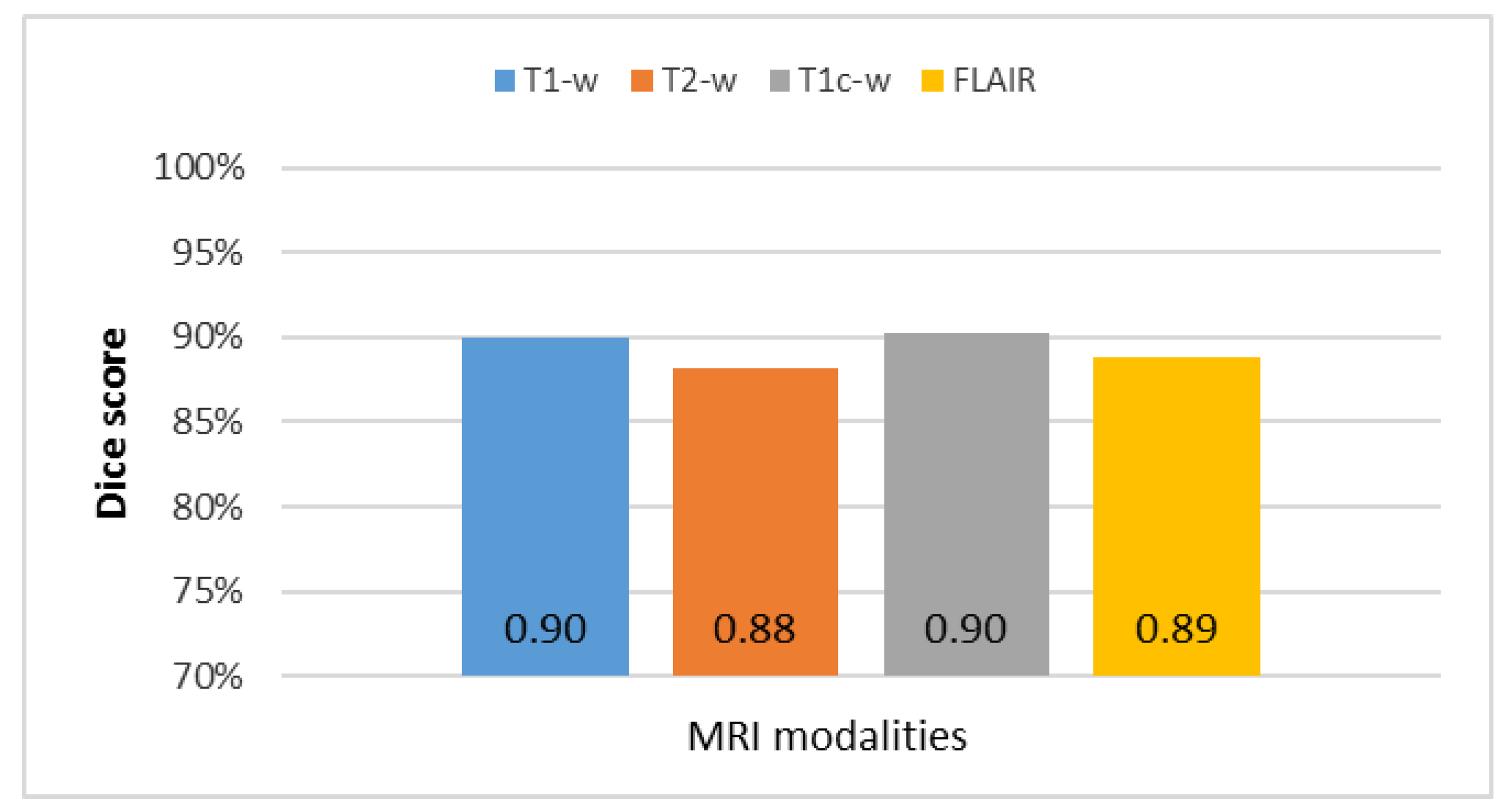
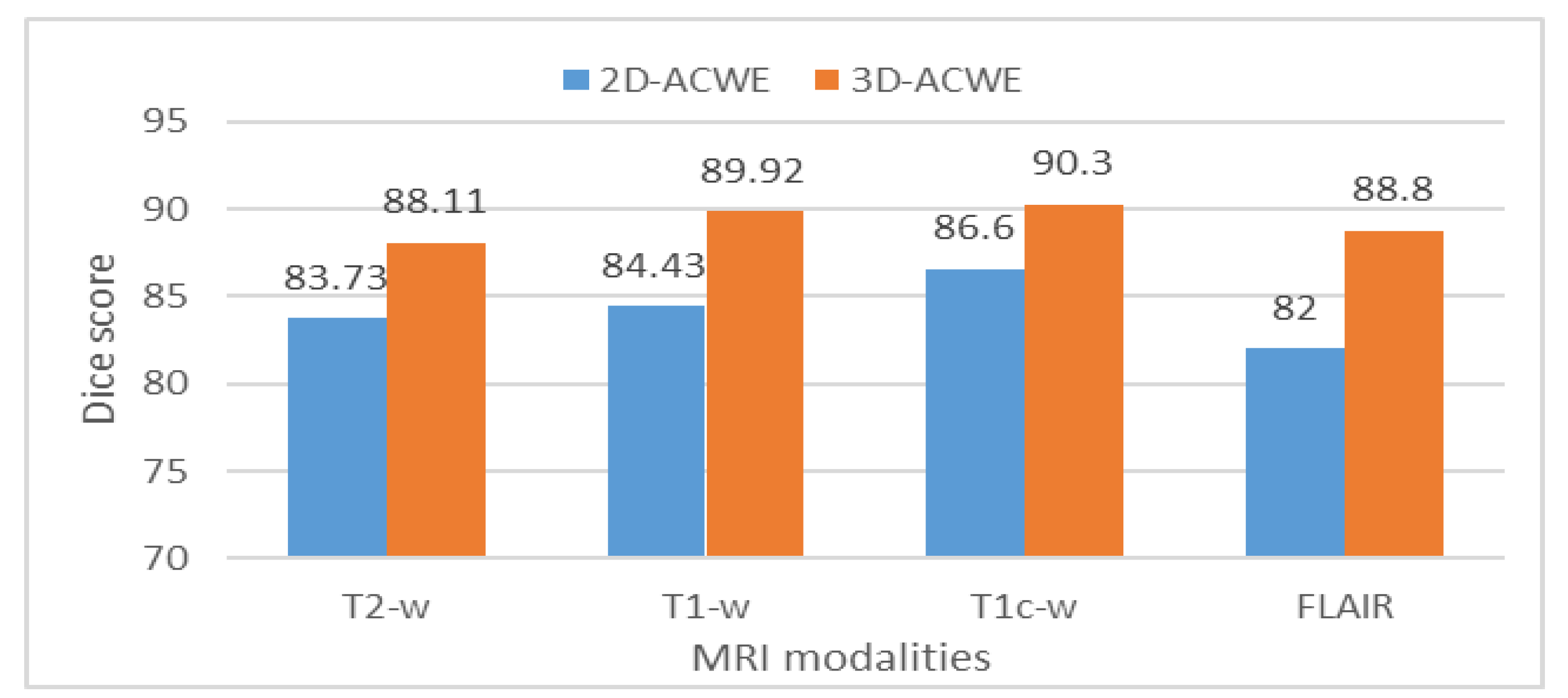
3DACWE	88.11% ± 4.4%	89.92% ± 4.9%	90.3% ± 3.6%	88.8% ± 6.9%

shows a comparison between the achieved mean Dice score and SD of 2DACWE and 3DACWE methods in segmenting images obtained under the four MRI modalities T2-w, T1-w, T1c-w, and FLAIR (Figure 13).

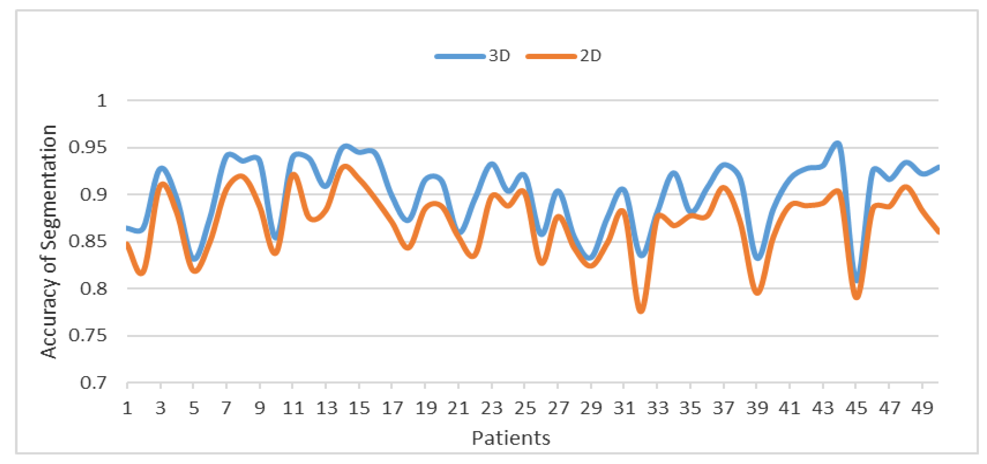
Figure 14 compares between the 3DACWE and 2DACWE segmentation results of the collected dataset. Notably, 3DACWE outweighs the 2DACWE method for all patients in the given dataset.

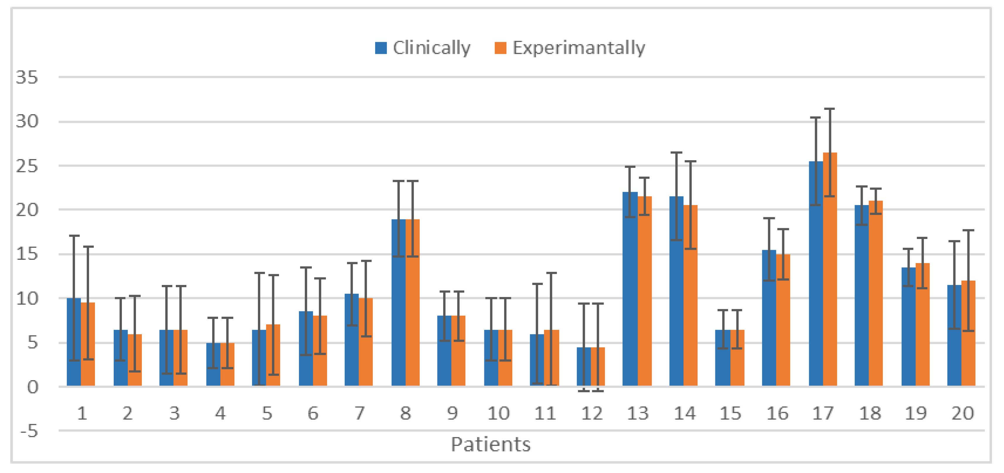
Figure 15 shows a comparison of the clinical and experimental identifications of the most relevant slices for the 20 pathological patients by measuring the means and SD between the two groups. Notably, the means and SD of the clinical and experimental tests are similar.

3.4. Discussion

The 3DACWE method was successfully applied to both the collected and standard datasets of BRATS 2013. The achieved Dice score of the collected dataset was 89% ± 4.7%, whereas the achieved Dice score of BRATS 2013 was 89.3% ± 4.2%. A major difficulty was encountered during white matter tumor segmentation because of the overlapping white and gray matter intensity distributions in such case. Some parts of the tumors in the gray matter were not distinguished because of restricted image resolution and the complex network of brain tissue with various shapes and sizes. These factors significantly affected a large number of voxels located on the tissue borders. Moreover, central tumor image intensity slightly differed from the peripheral tumor intensity. As such, the intensity near the borders can be considered similar to that of the gray matter. Consequently, the tumor and gray matter may be confused, and the peripheral tumor regions may be misclassified.

Tumor size affects segmentation accuracy, and errors usually occur at the tumor boundaries. Large brain tumors contain a high number of image pixels that can be misclassified. Moreover, large tumors likely ingress into the brain boundary and CSF fluid and render the precise determination of tumor boundary challenging. With regard to the overall executive processing time, the proposed system handled volumetric MRI data with different characteristics, such as number of slices and tumor size, type, boundary, and location. These characteristics make the overall segmentation process time consuming. Hence, the processing time of the proposed system was measured by second per MRI slice. Our proposed system required 243 s/MRI slice to run the segmentation.

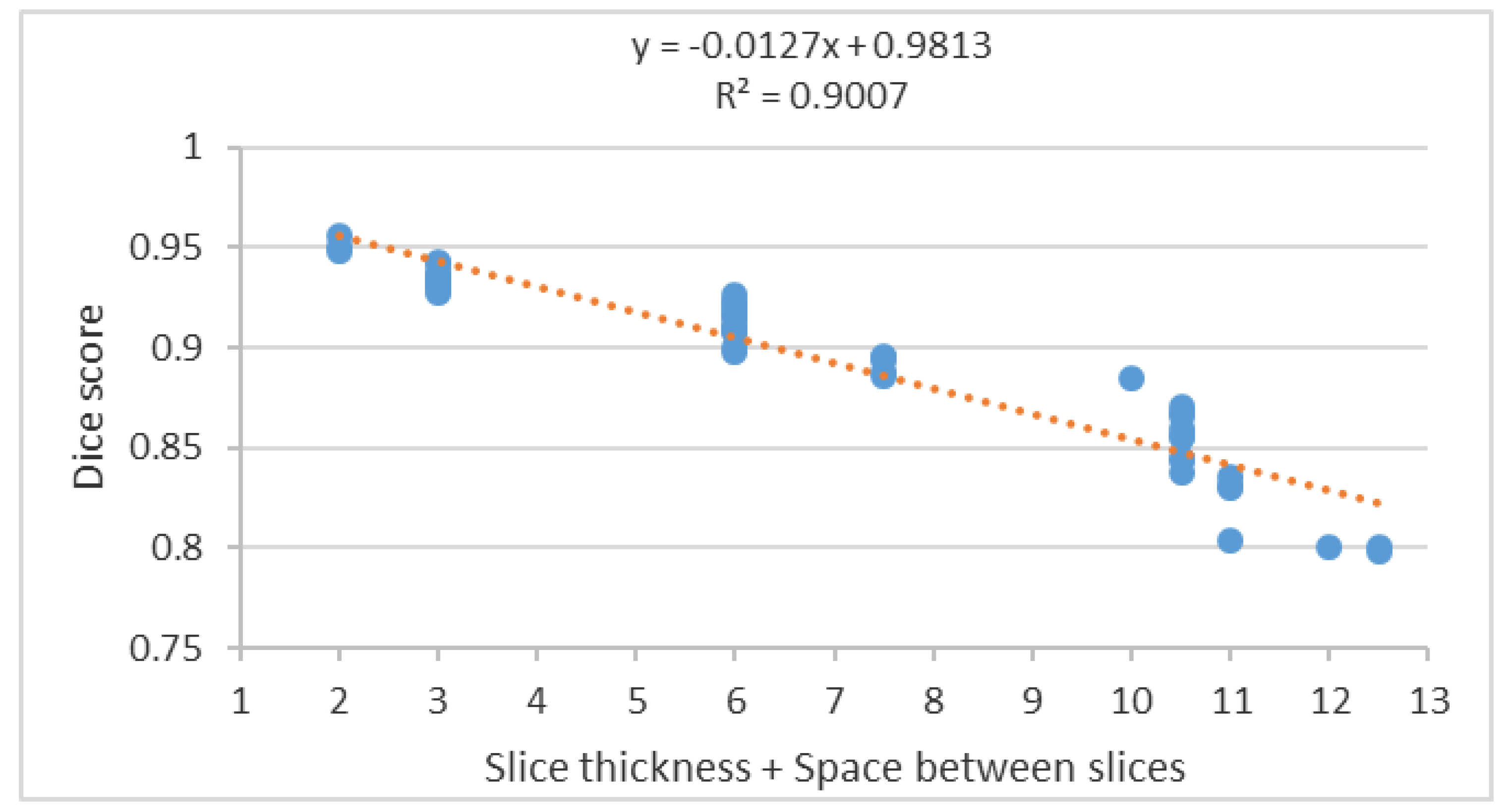
Segmentation accuracy decreased significantly with increasing slice thickness as shown in the scatter plot of the segmentation accuracy to the summation of slice thickness and space between slices (Figure 16).

The scatter plot in Figure 16 shows a negative correlation between the Dice score and the summation of the slice thickness and space between slices. Therefore, to achieve high segmentation accuracy, a reduction of the slice thickness and space between slices to a minimum is essential and diminishes the PV effect.

Table 5. Overview of the segmentation methods compared with the proposed system.

Reference	MRI Modalities	Approach	No. of Patients	Accuracy (100%)	Match (100%)	Jaccard (100%)	Dice (100%)
[33]	T1, T2, and PD	Fuzzy clustering	6	-	53–91	-	-
[41]	T1	Template-moderated classification	20	95	-	-	-
[42]	T1, and T1-c	Level-sets	5	-	-	85–93	-
[43]	T2	Generative model	3	-	-	59–89	-
[44]	T1, T1-C, T2, and FLAIR	Weighted aggregation	20	-	-	62–69	-
[12]	T1, T1-c, T2, and FLAIR	SVM	14	34–93	-	-	-
[45]	T1, T1-c, T2, and FLAIR	Generative model	25	-	-	-	40–70
Proposed System	T1, T1-c, T2, and FLAIR	3D-ACWE	50 (collected)	99.8 ± 0.2	85.4 ± 6.9	80.4 ± 7.4	89 ± 4.7
			25 (BRATS 2013)	99.9	91 ± 7.6	81 ± 6.8	89.3 ± 4.2

contains an overview of the segmentation methods demonstrated in [8].

4. Conclusions

Visual diagnosis of MRI scan images is subjective and highly dependent on clinician expertise. The proposed method offers a reduction of clinician evaluation time from 3–5 h to 5–10 min without significant reduction in the accuracy of the diagnosis. Indeed, the proposed method can recognize and segment MRI brain abnormality (tumor) on T2-w, T1-w, T1c-w, and FLAIR images. The 3DACWE segmentation technique reduces manual input, offers a rapid operation, and exhibits high accuracy compared with manual segmentation as evaluated using both the Al-Kadhimiya and BRATS 2013 datasets. We conclude that the 3DACWE method is effective in brain tumor segmentation because the approach does not only consider local tumor properties, such as gradients, but also relies on global properties, such as intensity, contour length, and region length. Although the achieved accuracy was high relative to those of other segmentation techniques, the 3DACWE was relatively slow for brain tumor segmentation. Such a slow pace was ascribed to the processing of a massive number of MRI slices of 512 × 512 pixel resolution with a high number of iterations used to attain the required accuracy.