
A New Bayesian Edge-Linking Algorithm Using Single-Target Tracking Techniques

Center for Information Security Technologies (CIST), Korea University, Seoul 02841, Korea
Symmetry 2016, 8(12), 143; https://doi.org/10.3390/sym8120143
Submission received: 31 July 2016
/
Revised: 14 November 2016
/
Accepted: 16 November 2016
/
Published: 1 December 2016
Abstract
:This paper proposes novel edge-linking algorithms capable of producing a set of edge segments from a binary edge map generated by a conventional edge-detection algorithm. These proposed algorithms transform the conventional edge-linking problem into a single-target tracking problem, which is a well-known problem in object tracking. The conversion of the problem enables us to apply sophisticated Bayesian inference to connect the edge points. We test our proposed approaches on real images that are corrupted with noise.
1. Introduction
Edge detection is a key and fundamental step in many computer vision and image-processing applications since it produces useful features of raw images. Edge detection takes a gray-scale image as input and generates a binary image map that includes black-and-white values at each pixel. Many researchers have devoted their efforts to inventing edge-detection algorithms.
Edge detection is based on the detection of abrupt local changes in the image intensity. In practice, edge models are classified according to their intensity profiles: step, ramp and roof. Given the edge model, edge detection involves three fundamental steps: image smoothing for noise reduction, detection of edge points and edge localization [1]. That is, we first reduce the noise in images by using several low-pass filters [2,3] in the image smoothing for noise reduction step. The detection of edge points step is a local operation that extracts all points that are potential candidates for edge points. In other words, the algorithms consider all of the points and then use thresholds, a histogram, gradients and zero crossing to identify promising edge points [4,5,6]. The last step is edge localization, the objective of which is to select from the candidate edge points only those points that would be meaningful to build the desired features. However, it is not straightforward to obtain the complete set of desired features even after the above three steps. Although edge detection should yield sets of pixels that only coincide with edges, the actual underlying edges are seldom characterized by the detected pixels because of unwanted noise in raw images, spurious breaks in the edges and improperly-chosen threshold values. Therefore, edge-linking or boundary detection/tracing algorithms often follow edge detection to eventually recognize the simplified and salient object of interest from the image. Various algorithms have been developed to connect the detected edge points. Broken edges are extended along the directions of their respective slopes by using an (adaptive) morphological dilation operation [7,8]. Multiple resolution and hierarchical approaches to edge detection were also proposed by [9,10]. Another well-known approach for edge linking is the Hough transform [11]. The graph search problem with the algorithm has also been used to link edges [12]. Probabilistic relaxation techniques have been applied to label edges for boundary tracing, as well [13,14,15,16]. A predictive edge-linking algorithm was also developed by considering the prediction generated by past movements [17]. In addition to these, many other approaches to developing edge-linking algorithms have been proposed [18,19,20,21]. However, most algorithms are not effective for general-purpose usage, and they are highly dependent on the data and applications because of the presence of noise and long interruptions (the existence of occlusions).
Therefore, we propose a new approach to connect the edge points to create meaningful longer edges even in the presence of a large amount of noise, unwanted interruptions and long occlusions. Our idea to link the detected points is to combine our linking edges with data association in the object target tracking methodology. The data association technique in target tracking is commonly used to identify detected points of objects in a cluttered environment, and it classifies observations as being either target oriented or non-target oriented. That is, such object tracking schemes can be applied to classify the detected points into desired edges or unwanted clutter. In the work presented in this paper, the target tracking method for boundary determination is designed as part of a Bayesian scheme, and the posterior distribution is the objective function with the shape prior in a Markov random field (MRF).
The contributions of our paper are fourfold: (1) introducing a new probabilistic relaxation technique using single-target tracking techniques; (2) overcoming multiple occurrences of noise and long occlusions; (3) designing three efficient statistical methodologies; and (4) application to interactive segmentation.
This paper consists of several sections. Section 3 presents background knowledge related to the techniques that are used in this paper. After first explaining the intuitive idea of our approach in Section 2, various algorithms are proposed in Section 4. Afterwards, we conclude with our results and a related discussion.
2. Motivation (Idea)
In this paper, we propose a new approach to linking edges based on our idea to introduce single-target tracking algorithms. Target tracking algorithms have found use in many application domains of computer vision and image processing [22,23,24,25,26]. Given the raw image in Figure 1a, we have a binary image in Figure 1b after applying several detection algorithms, such as Canny and Sobel. Of course, advanced statistical detection algorithms can be applied [27,28]. Here, if we want to obtain the boundary of the triangle from the detected points, we can click any point inside of the polygon in an interactive way [29]. We name this point an origin. Then, we obtain T lines from the binary image in a radial way using Bresenham’s line-drawing algorithm, as shown in Figure 1c. This is similar to the approach followed in the star convexity shape prior approach [30]. Each line can cross the detected points that are potential edge candidates, and we set the crossed points to be the measurements of our interest in the tracking system. That is, each line in Figure 1c is the same as the time slot in the tracking domain, as shown in Figure 1d. Now, the radial distance (r) of the crossed points represents the value of the observations. Finally, we can obtain several observations (labeled ‘x’ in Figure 1) with T discrete time slots since T intersections are taken into account in the image. After transforming the two-dimensional image into a one-dimensional radial space, we apply a conventional single-target tracking technique since the boundary of any object will be constructed from the obtained trajectory or data association represented by the set of red circles in Figure 1d.
3. Mathematical Background
As described in Section 2, boundary tracing is performed with the single-target tracking technique that is popularly used in highly noisy surveillance systems. Since our tracking model is based on an off-line system, we use the idea of Markov chain Monte Carlo data association (MCMCDA) [31] to provide highly accurate data association for edge linking. MCMCDA uses data association to partition the measurements into two sets of data: target-oriented measurements and non-target oriented measurements (clutter). After this data association process, the single-target tracking problem becomes much simpler and straightforward to address [31]. Let the unobserved stochastic process with hidden states for , , be modeled as a Gaussian Markov random field (GMRF) process of transition probability for the system prior, where is a set of the neighbors of the t-th state.
3.1. Gaussian Markov Random Field
A shape prior is now commonly used for segmenting images in image processing and computer vision [32].
A Markov random field (MRF) is often used in the segmentation of images in image processing and computer vision. For instance, MRF models the relation of neighboring pixels to the coloring foreground and background using a mathematical model, such as the Ising or Potts model [33,34,35]. There are alternative uses of MRF in computer vision. MRF has been used for the object shape prior, which is used for Bayesian object recognition [36,37]. Our work is also based on the use of a shape prior.
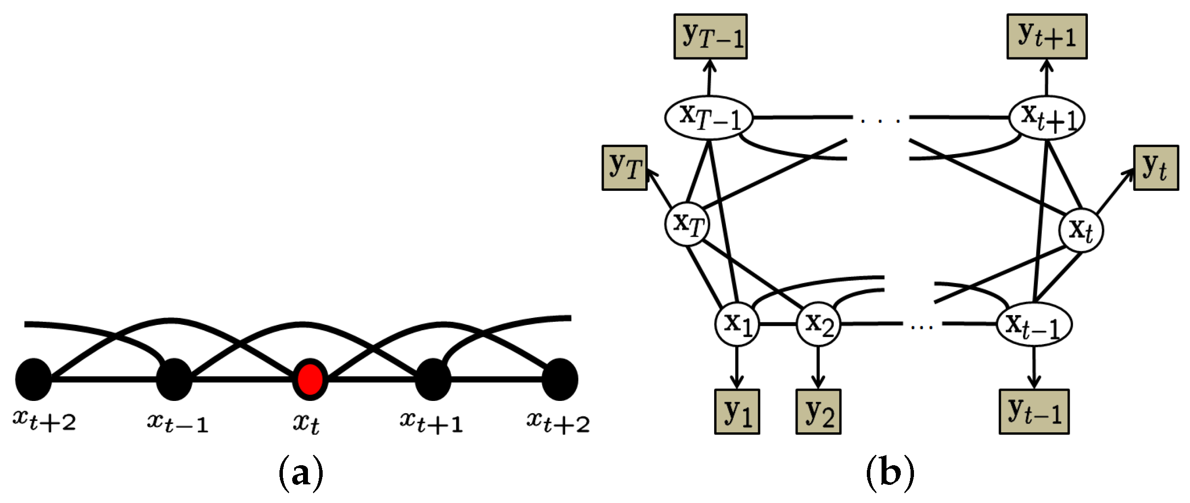
Assume that there is a graphical model that consists of a set of states with the second order Gaussian Markov random field (GMRF) [38] representation in Figure 2a.
Given the GMRF model, we have an interesting mathematical form of the prior as Equation (1):
where , and is a circulant matrix defined by:
3.2. Circular State Space Model
We assume the likelihood for the target-oriented measurements as follows , and the non-target-oriented measurements follow a uniform distribution since there is no prior information. We have the following state and measurement space models in a time series, as shown in Figure 2b. Given the GMRF prior and likelihood function, we have . We finally have a marginalized likelihood for the circular state space model with observations in the time series by:
3.3. Data Association for Single-Object Tracking
By assuming that the time series contains a single track, then each observation can be assigned to one of the following cases: the observation is an element of a set of clutter, i.e., , or the observation is a target-oriented signal, i.e., . Therefore, data association partitions the measurements into target-oriented observations and clutter . The motivation of our proposed tracking algorithm is now to search for an appropriate single track .
Note that we simplified the notation of the observations by and for since it is cyclic. Suppose that is a configuration of , and it is a collection of partitions of . For , we have , where and , is a set of clutter, false alarms, for , and , where is the minimum length of the proposed track. The cardinality of the set is denoted by . Let be the set of unknown environmental parameters (EPs), where is the transpose operator. In the EPs, is the detection probability, and is the false alarm rate per unit time. Our interest is to generate samples from a stationary posterior distribution for the configuration ,
The conditional posterior has the form,
where follows a Gaussian Markov random field (GMRF) prior.
As mentioned in connection with the original MCMCDA, we can use fixed environmental parameters (EPs), θ. When they are known, we can sample only over the conditional posterior distribution, since the underlying trajectory is marginalized as in Equation (2). Therefore, the stationary posterior distribution of our interest is:
where and , denote the Bernoulli and Poisson distributions, respectively. Here, R is the maximum distance from the origin for all measured observations, and and denote the detection probability and the false alarm occurrence rate . The observations are divided into two sets: and , which are the sets of observations containing the clutter and targets, respectively. In this equation, the parameters, deterministically obtained when the model configuration is proposed, are given by the number of detections at time t, , the number of undetected targets at time t, , and the number of false alarms at time t, . In addition, we need to consider a special case in which there are no detected observations for certain sequential slots in order to design occlusions for the boundary. For instance, we may not have any observations at times a and b in data association; thus, let be a set of the time indexes of the undetected observations. Now, our likelihood can be slightly changed by applying marginalization, and denotes ‘not ’, such that:
4. Proposed Approach
4.1. Improved Posterior with Marginalization of the EPs
The unknown parameters of our interest are both the configuration and the environmental parameters θ. Their prior distribution is decomposed by where:
and and are assumed to be independent. Given the conjugate prior distribution of the EPs and configuration, we have the marginalized posterior,
where:
and is assumed to be a uniform distribution since we do not have any prior information thereof. The detailed derivation is shown in Appendix A.1.
Finally, the log of the marginalized posterior is:
where
4.2. Approach Based on the Metropolis–Hastings Algorithm
Markov chain Monte Carlo (MCMC) is one of the most intuitive statistical approaches to constructing a target posterior, and it is applied to image processing [39,40,41]. We implemented several types of moves for the Metropolis–Hastings (MH) update for linking edges: (a) pop: an observation moves from to ; that is, an observation that was previously considered as a target-oriented one is now considered in a non-target observation; (b) push: an observation moves from to ; i.e., an observation that was previously considered as a non-target-oriented observation is re-categorized as a target-oriented observation; and (c) swap: for time t, if we have a target-oriented observation and we can choose a non-target-oriented observation for and , then, we exchange them in the sets. That is, the updated configuration has two updated sets: and . We have an acceptance probability for the Metropolis–Hastings algorithm: .
4.3. Gibbs Sampler-Based Approach
Here, given the mathematical model, we can calculate the posterior distribution of each case of data association at time t, and a Gibbs sampler can generate the samples from the pre-calculated posterior distribution. From this point of view, we first introduce an auxiliary random variable that identifies the index of the target-oriented observation at time t from the data association for , i.e., , where is the number of measurements at time t. Here, represents that no target-oriented measurement is detected, and represents that the i-th observation is detected and is a target-oriented signal at time t. Now, our interest is to generate samples from the joint full posterior distribution of , , rather than , since the configuration reconstructed by is equivalent to the configuration, , which has been referred to in the previous sections. We draw a sample from the conditional posterior as in Algorithm 1 by for time t. Therefore,
and it is directly estimated by:
where the configuration is constructed with .
| Algorithm 1 Gibbs sampler-based approach. | |
| 1: | Let be a vector with non-negative integers s.t. for all . |
| 2: | for to do |
| 3: | for to T do |
| 4: | for to do |
| 5: | and make from the . |
| 6: | end for |
| 7: | Calculate the posterior |
| 8: | Draw a sample from the conditional posterior by |
| 9: | end for |
| 10: | Reconstruct using and find the best configuration with the MAP estimate. |
| 11: | end for |
4.4. Variational Bayes Using Mean-Field Approximation with Pseudo-Integration
Variational Bayes (VB) is a particular variational method that aims to find some approximate joint distribution over the hidden variable to approximate the true joint distribution by minimizing the Kullback–Leibler (KL) distance (relative entropy), . In this case, has a simpler form than true distribution , and the mean-field form is used to factorize the joint into single-variable factors, . In VB, we wish to obtain a set of distributions to minimize the KL distance,
We can assume that the factorized form via the mean field follows a multinomial distribution, and then, we have:
where is the multinomial distribution with control parameter and for all . An iterative update equation for the factorized single-value form provides:
Unfortunately, the right-most form of the above equation is not easily estimated, since it does not have a conjugate form; hence, we introduce the second approximated function:
where are the fixed values that are estimated from the previous step in a way similar to MAP or Gibbs samplers. Given this second approximation, we rewrite:
Here, the second term on the right-hand side is the likelihood we already defined in Equation (4), such that:
Thus, we can calculate the probability mass function for the likelihood directly, and we assign it as:
Then, we write the marginal likelihood as a multinomial distribution by:
Therefore, we write:
and:
where for all and . Here, is the newly-updated distribution.
The algorithm of the variational approach is decribed in Algorithm 2.
| Algorithm 2 Variational Bayes approach. |
| 1: Let be a vector with non-negative integers s.t. for all . |
| 2: Set for all . |
| 3: Reconstruct using , and set . |
| 4: while (convergence) do |
| 5: . |
| 6: for to T do |
| 7: for to do |
| 8: , and make from . |
| 9: end for |
| 10: Calculate for all . |
| 11: Update for all . |
| 12: Normalize the updated distribution, . |
| 13: Obtain , and update . |
| 14: end for |
| 15: Reconstruct using , and find the best configuration using the MAP estimate. |
| 16: end while |
4.5. Variance Estimation Using Markov Chain Monte Carlo
The next question is how to estimate κ and τ. Unfortunately, neither of these parameters has any closed form, so that we cannot draw the samples using the Gibbs sampler. Alternatively, we can estimate them by using two approaches: (a) the Metropolis–Hastings (MH) algorithm; and (b) prior processing in the training step using fast heuristic algorithms, such as the EMapproach. In this paper, we use MCMC to ensure consistency in the Monte Carlo approach since the Gibbs sampler is a type of Monte Carlo.
Samples of the parameters are drawn using a standard MH algorithm, such that the unknown parameters are jointly updated according to an acceptance probability:
where .
5. Results
We performed simulations on raw images to evaluate our proposed algorithms. We compared the performance with a popularly-used boundary tracing technique that is a built-in function, “bwtraceboundary”, and our proposed three algorithms. Note that the boundary tracing approach is not used for segmenting objects in an image; instead, it is used for linking points. However, we chose this algorithm for the comparison since our approach mainly involves linking edge points in order to segment the objects. We used the following settings for our proposed algorithms: , , and .
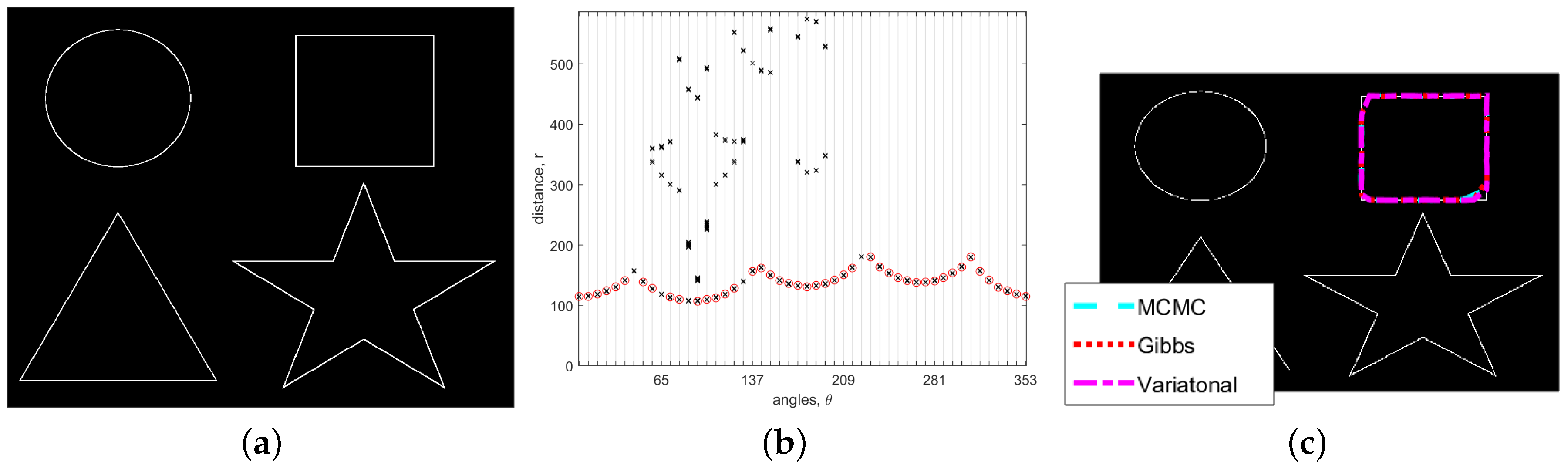
5.1. Noise-Free Image
The simulation results we obtained for a noise-free image are as shown in Figure 3. This figure displays three sub-figures: the detected points (left), the trajectory we estimated from the edge points using variational inference (center) and the object segmented using the three proposed approaches (right). Using the interactive segmentation scheme [42,43], we clicked the center of the square in Figure 3a. As we can see in Figure 3b, whereas the detected edge points of uninteresting objects, including “star”, “circle,” and “triangle”, are considered as clutter, the edge points of the square are processed as significant signals with a long trajectory in our proposed approaches. Thus, for a noise-free image, we can obtain proper segmentation using our three proposed approaches as shown in Figure 3c. The elapsed times for this noise-free image are (MCMC), (Gibbs) and (variational Bayes). As expected, the variational Bayes approach is more efficient than the other two approaches for noise-free image segmentation.
5.2. Images with Occlusion
Image segmentation is known not to be straightforward for images in which occlusion exists. In order to evaluate the performance of our proposed approaches, we generated a synthetic example with occlusion as shown in Figure 4a. In this figure, the square in the black-and-white image includes occlusion. The red circles in the central sub-figure signify the observations associated with the restored trajectory using variational inference. This figure also shows interesting results in that observations in the corner of the square are not detected in the trajectory, even though they are well detected in the noise-free image in Figure 3a. This is because the observations at the corners are considered to be clutter since the occlusions introduce additional uncertainty in the trajectory.
5.3. Image Segmentation with Varying Noise Levels
The final aspect we need to investigate as part of our performance evaluation is to check the extent to which the proposed approaches accurately segment objects in an image with varying noise levels. Thus, we added salt and pepper noise at a noise level of .
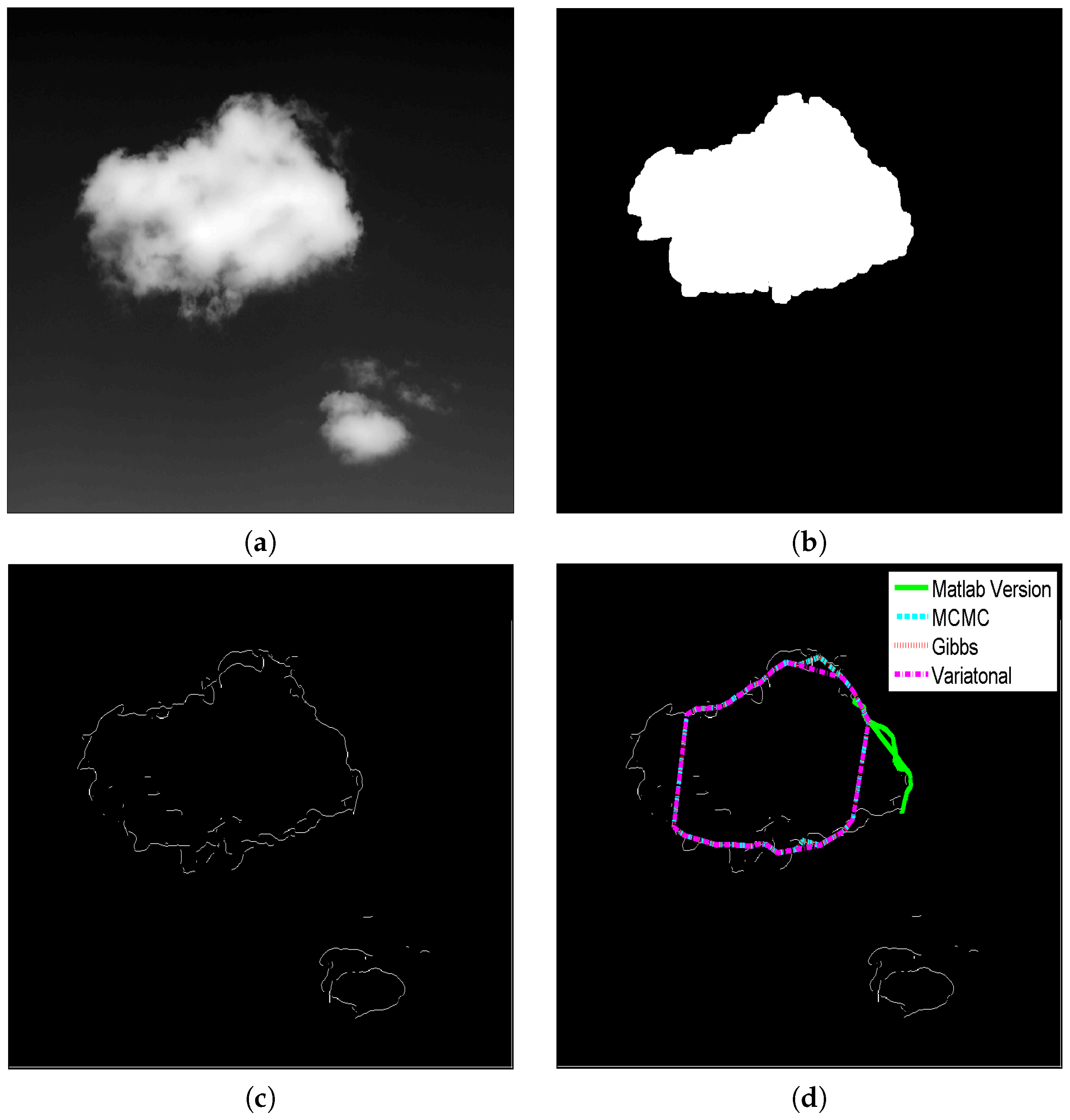
Figure 5 shows (a) the raw image without any added noise ; (b) hidden true segmentation; (c) detected points obtained using the “Sobel” detector; and (d) the linked boundary. As can be seen in Figure 5c, many detected points are not connected, although the raw image does not contain any additional noise. We evaluated the performance of our algorithm by comparing two measures: the averaged values and standard deviations of overlapping rates and execution times with 10 runs. The overlapping rate is the similarity between the hidden true segmentation in Figure 5e and the region that is reconstructed from the detected trajectories. Let and be the hidden true segmentation and the reconstructed polygon with a small number of detected observations. The similarity is calculated by . Note that has a value between zero and one. As the similarity approaches one, the reconstructed polygon increasingly takes on the desired, hidden true segmentation.
The segmentation results obtained using four different algorithms are shown in Figure 6. As shown in this figure, the “bwtraceboundary” in MATLAB performed very poorly in all cases because it cannot overcome noise. However, our proposed approach performs well even in a severely-cluttered environment as in . Another interesting finding is the ability of the MCMC-based approach to reliably construct the boundary such that the edges seem invariant. However, the Gibbs sampling and variational Bayes (VB) approaches are adversely affected by the noisy data and perform unstable segmentation. Table 1 presents a more quantitative comparison in terms of the overlapping rate and execution time. As can be seen in this table, MCMC outperforms the other approaches in all cases, and it provides stable results even for . As we expected, the performance of all approaches also tends to decrease as more noise is added. Since MCMC and the Gibbs sampler are Monte Carlo simulations, they are rather slower than “bwtraceboundary” and VB. The last important finding is that VB is a practically efficient algorithm for small values of since it provides a high overlapping rate and its execution time is relatively short compared to that of the Monte Carlo simulations.
5.4. Application to More Complicated Raw Images
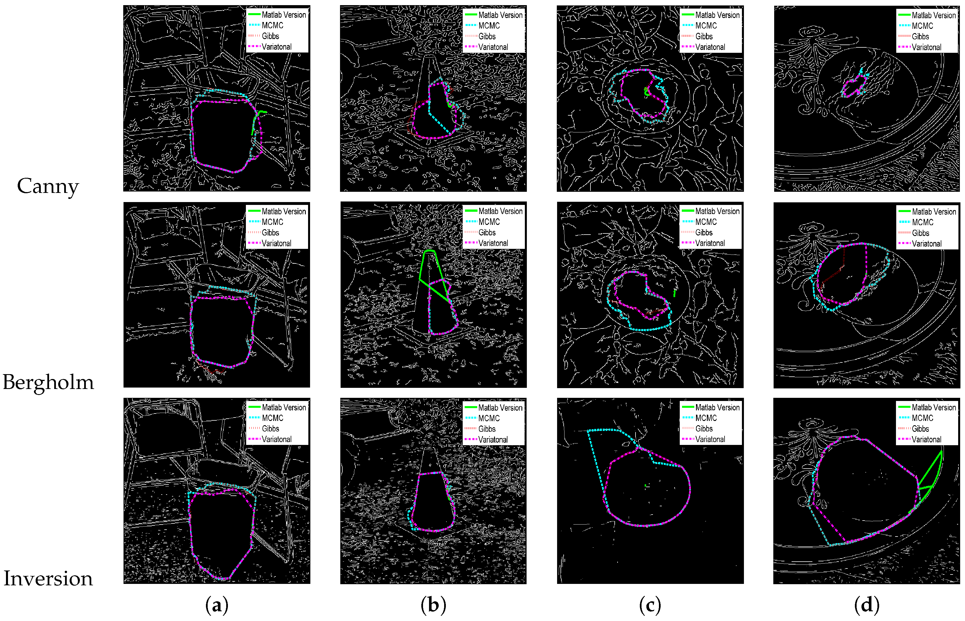
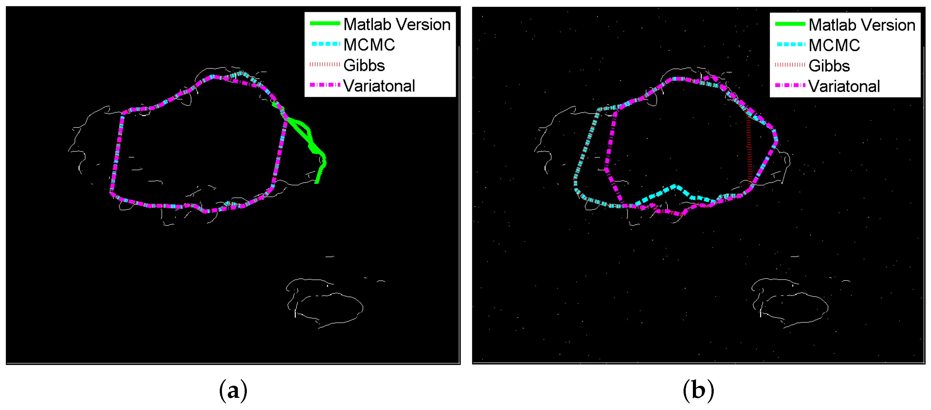
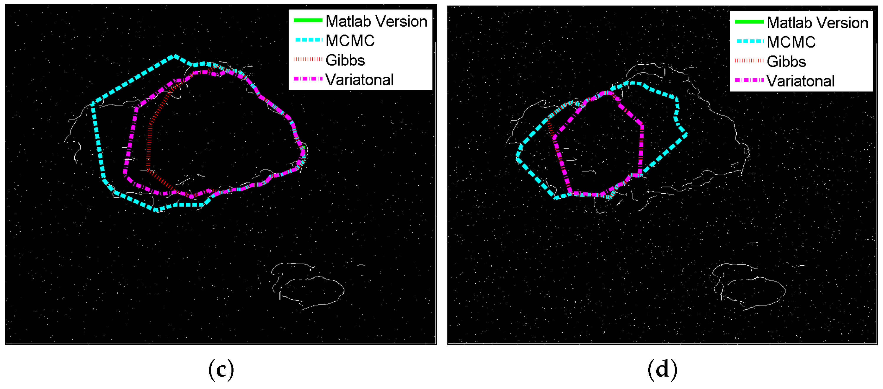
We also tested our proposed approaches on several natural images that were obtained from a few image databases [29,44]. Figure 7 shows the segmentation results processed by the “bwtraceboundary” function and our proposed three approaches. We obtained the edge points from the raw image by using Gaussian convolution and a Canny detection [6]. The first, second, third and fourth rows represent the natural images, edge points obtained by the Canny detection, trajectories associated by variational inference and the final segmentation using the four different approaches.
Figure 7 shows that our proposed approaches outperform “bwtraceboundary” in the segmentation procedure. In addition, the segmentation results of the MCMC simulation are more rigid than those obtained using the Gibbs and variational approaches. We also compared the elapsed times for all approaches. Table 2 indicates that ’.
We also evaluated the performance of our proposed approaches by changing the detection algorithms. Figure 8 shows the segmentation results for the detected points, which were obtained by the Canny, Bergholm and inversion detection algorithms. It is obvious that our proposed approaches depend on the performance of the edge detection algorithm in use. For instance, the objects in (b), (c) and (d) are well segmented when the inversion detection algorithm is used.
6. Discussion
Apart from the superior performance of our proposed approach in terms of the segmentation of some real images, there are several issues that need to be improved. First, our proposed approach samples the intersecting lines in a radial way such that polygons with a concave form may not be appropriately segmented. Instead of obtaining the concave shape, our proposed approaches are likely to partition the desired concave polygon into several unwanted smaller convex polygons; Second, there are several hyper-parameters that should be carefully selected: κ, τ and for the coefficients of the second order GMRF. Unfortunately, these hyper-parameters are very sensitive in the sense that if they are poorly selected, our proposed approaches do not work. Therefore, we need to conduct research on how to automatically select the hyper-parameters used in learning or estimation frameworks; Third, the current approaches do not guarantee stability as they rely on varying origins. The location of the origin determines the velocity and acceleration of the trajectory, which means that κ and τ would have to be changed with varying location; Last, we need to improve our proposed approaches to enable them to process multiple objects since the current algorithms only have the ability to accommodate single objects using single-target tracking.
7. Conclusions
We introduced a new scheme capable of embedding single-target tracking algorithms, to connect edge points for longer salient edges. Conventional approaches for linking edges are mostly based on the connection of neighboring points rather than global patterns. Therefore, these approaches perform very poorly in the presence of unwanted noise, interruptions and occlusions. However, we can overcome these problems by introducing a probabilistic target-tracking scheme, such as that typically used in cluttered surveillance systems. That is, we converted the edge-linking problem into a target-tracking problem. Given this tracking scheme, we also developed three different algorithms: MCMC, a Gibbs sampler and variational Bayes. MCMC outperforms the other approaches in most cases, although the variational Bayes algorithm seems practically efficient, because it has reasonable accuracy and is computationally effective.
Acknowledgments
The author is supported by a new faculty research grant from Korea University.
Conflicts of Interest
The author declares no conflict of interest.
Appendix A
Appendix A.1. Marginalized Posterior
Given the prior distribution of the EPs and configuration, we can build the marginalized posterior,
where , , , and is assumed to be a uniform distribution, since we do not have any prior information thereof. Finally, the log of marginalized posterior is , where
Appendix A.2. MATLAB Source Code
A MATLAB source code of the proposed algorithms can be downloaded from the website [45].
References
- Gonzalez, R.C.; Woods, R.E. Digital Image Processing, 2nd ed.; Addison-Wesley Longman Publishing Co., Inc.: Boston, MA, USA, 2001. [Google Scholar]
- Lebrun, M.; Buades, A.; Morel, J. A Nonlocal Bayesian Image Denoising Algorithm. SIAM J. Imaging Sci. 2013, 6, 1665–1688. [Google Scholar] [CrossRef]
- Yoon, J.W. Statistical denoising scheme for single molecule fluorescence microscopic images. Biomed. Signal Proc. Control 2014, 10, 11–20. [Google Scholar] [CrossRef]
- Otsu, N. A Threshold Selection Method from Gray-Level Histograms. IEEE Trans. Syst. Man Cybern. 1979, 9, 62–66. [Google Scholar] [CrossRef]
- Marr, D.; Hildreth, E. Theory of Edge Detection. Proc. R. Soc. Lond. Ser. B Biol. Sci. 1980, 207, 187–217. [Google Scholar] [CrossRef]
- Canny, J. A Computational Approach to Edge Detection. IEEE Trans. Pattern Anal. Mach. Intell. 1986, PAMI-8, 679–698. [Google Scholar] [CrossRef]
- Meyer, F.; Beucher, S. Morphological segmentation. J. Vis. Commun. Image Represent. 1990, 1, 21–46. [Google Scholar] [CrossRef]
- Shih, F.Y.; Cheng, S. Adaptive mathematical morphology for edge linking. Inf. Sci. 2004, 167, 9–21. [Google Scholar] [CrossRef]
- Cook, G.W.; Delp, E.J. Multiresolution sequential edge linking. In Proceedings of the 1995 International Conference on Image Processing (ICIP), Washington, DC, USA, 23–26 October; IEEE: New York, NY, USA, 1995; pp. 41–44. [Google Scholar]
- Casadei, S.; Mitter, S.K. A hierarchical approach to high resolution edge contour reconstruction. In Proceedings of the 1996 IEEE Computer Society Conference on Computer Vision and Pattern Recognition (CVPR ’96), San Francisco, CA, USA, 18–20 June 1998; IEEE: New York, NY, USA, 1998; pp. 149–154. [Google Scholar]
- Herout, A.; Dubská, M.; Havel, J. Review of Hough Transform for Line Detection. In Real-Time Detection of Lines and Grids; SpringerBriefs in Computer Science; Springer: London, UK, 2013; pp. 3–16. [Google Scholar]
- Farag, A.A.; Delp, E.J. Edge linking by sequential search. Pattern Recognit. 1995, 28, 611–633. [Google Scholar] [CrossRef]
- Hancock, E.R.; Kittler, J. Edge-labeling using dictionary-based relaxation. IEEE Trans. Pattern Anal. Mach. Intell. 1990, 12, 165–181. [Google Scholar] [CrossRef]
- Christmas, W.J.; Kittler, J.; Petrou, M. Structural matching in computer vision using probabilistic relaxation. IEEE Trans. Pattern Anal. Mach. Intell. 1995, 17, 749–764. [Google Scholar] [CrossRef]
- Feng, J.; Shi, Y.; Zhou, J. Robust and Efficient Algorithms for Separating Latent Overlapped Fingerprints. IEEE Trans. Inf. Forensics Secur. 2012, 7, 1498–1510. [Google Scholar] [CrossRef]
- Mirmehdi, M.; Petrou, M. Segmentation of color textures. IEEE Trans. Pattern Anal. Mach. Intell. 2000, 22, 142–159. [Google Scholar] [CrossRef]
- Akinlar, C.; Chome, E. PEL: A Predictive Edge Linking algorithm. J. Vis. Commun. Image Represent. 2016, 36, 159–171. [Google Scholar] [CrossRef]
- Yang, X.; Liu, H.; Latecki, L.J. Contour-based object detection as dominant set computation. Pattern Recognit. 2012, 45, 1927–1936. [Google Scholar] [CrossRef]
- Jevtic, A.; Melgar, I.; Andina, D. Ant based edge linking algorithm. In Industrial Electronics, 35th Annual Conference of IEEE Industrial Electronics; IEEE: New York, NY, USA, 2009; pp. 3353–3358. [Google Scholar]
- Wang, Z.; Zhang, H. Edge linking using geodesic distance and neighborhood information. In Proceedings of the IEEE/ASME International Conference on, Advanced Intelligent Mechatronics (AIM 2008), Xi’an, China, 2–5 July 2008; IEEE: New York, NY, USA, 2008; pp. 151–155. [Google Scholar]
- Ghita, O.; Whelan, P.F. Computational approach for edge linking. J. Electron. Imaging 2002, 11, 479–485. [Google Scholar] [CrossRef]
- Isard, M.; Blake, A. Contour Tracking by Stochastic Propagation of Conditional Density; Springer: Berlin/Heidelberg, Germany, 1996; Volume 1, pp. 343–356. [Google Scholar]
- Isard, M.; Blake, A. A mixed-state Condensation tracker with automatic model-switching. In Proceedings of the Sixth International Conference on Computer Vision, Bombay, India, 7 January 1998; IEEE: New York, NY, USA, 1998; pp. 107–112. [Google Scholar]
- Isard, M.; Blake, A. A smoothing filter for Condensation. In Proceedings of the 5th European Conference Computer Vision, Freiburg, Germany, 2–6 June 1998; Springer: Berlin/Heidelberg, Germany, 1998; Volume 1, pp. 767–781. [Google Scholar]
- Zhang, S.; Zhou, H.; Jiang, F.; Li, X. Robust Visual Tracking Using Structurally Random Projection and Weighted Least Squares. IEEE Trans. Circuits Syst. Video Technol. 2015, 25, 1749–1760. [Google Scholar] [CrossRef]
- Zhou, H.; Taj, M.; Cavallaro, A. Target Detection and Tracking With Heterogeneous Sensors. IEEE J. Sel. Top. Signal Proc. 2008, 2, 503–513. [Google Scholar] [CrossRef]
- Lim, J.; Zitnick, C.L.; Dollár, P. Sketch Tokens: A Learned Mid-level Representation for Contour and Object Detection. In Proceedings of the Computer Vision and Pattern Recognition (CVPR), Portland, OR, USA, 23–28 June 2013.
- Marimont, D.; Rubner, Y. A probabilistic framework for edge detection and scale selection. In Proceedings of the Sixth International Conference on Computer Vision, Bombay, India, 7 January 1998; IEEE: New York, NY, USA, 1998; pp. 207–214. [Google Scholar]
- Gulshan, V.; Rother, C.; Criminisi, A.; Blake, A.; Zisserman, A. Geodesic Star Convexity for Interactive Image Segmentation. In Proceedings of the IEEE Conference on Computer Vision and Pattern Recognition, San Francisco, CA, USA, 13–18 June 2010.
- Veksler, O. Star shape prior for graph-cut image segmentation. In Proceedings of the 10th European Conference on Computer Vision (ECCV), Marseille, France, 12–18 October 2008; Springer: Berlin/Heidelberg, Germany, 2008; pp. 454–467. [Google Scholar]
- Oh, S.; Russell, S.J.; Sastry, S. Markov Chain Monte Carlo Data Association for Multi-Target Tracking. IEEE Trans. Autom. Control 2009, 54, 481–497. [Google Scholar]
- Chen, S.; Cremers, D.; Radke, R.J. Image Segmentation with One Shape Prior - A Template-based Formulation. Image Vis. Comput. 2012, 30, 1032–1042. [Google Scholar] [CrossRef]
- Barker, S.; Rayner, P. Unsupervised image segmentation using Markov random field models. Pattern Recognit. 2000, 33, 587–602. [Google Scholar] [CrossRef]
- Celeux, G.; Forbes, F.; Peyrard, N. EM-Based Image Segmentation Using Potts Models with External Field; Rapport de Recherche RR-4456; INRIA: Le Chesnay, France, 2002. [Google Scholar]
- Brault, P.; Mohammad-Djafari, A. Unsupervised Bayesian wavelet domain segmentation using Potts-Markov random field modeling. J. Electron. Imaging 2005, 14, 043011. [Google Scholar]
- Rue, H.; Syversveen, A.R. Bayesian object recognition with Baddeley’s delta loss. Adv. Appl. Probab. 1988, 30, 64–88. [Google Scholar] [CrossRef]
- Chen, S.; Radke, R. Level set segmentation with both shape and intensity priors. In Proceedings of the 2009 IEEE 12th International Conference on Computer Vision, Kyoto, Japan, 27 September–4 October 2009; IEEE: New York, NY, USA, 2009; pp. 763–770. [Google Scholar]
- Rue, H.; Held, L. Gaussian Markov Random Fields: Theory and Applications; Monographs on Statistics and Applied Probability; Chapman & Hall: London, UK, 2005; Volume 104. [Google Scholar]
- Fan, A.; Fisher, J., III; Wells, W., III; LEvitt, J.; Willsky, A. MCMC Curve Sampling for Image Segmentation. In International Conference on Medical Image Computing and Computer-Assisted Intervention; Springer: Berlin/Heidelberg, Germany, 2007; pp. 477–485. [Google Scholar]
- Chang, J.; Fisher, J.W., III. Efficient MCMC Sampling with Implicit Shape Representations. In Proceedings of the IEEE Computer Vision and Pattern Recognition (CVPR), Colorado Springs, CO, USA, 20–25 June 2011.
- Zhou, H.; Li, X.; Sadka, A.H. Nonrigid Structure-From-Motion From 2-D Images Using Markov Chain Monte Carlo. IEEE Trans. Multimed. 2012, 14, 168–177. [Google Scholar] [CrossRef]
- Panagiotakis, C.; Papadakis, H.; Grinias, E.; Komodakis, N.; Fragopoulou, P.; Tziritas, G. Interactive image segmentation based on synthetic graph coordinates. Pattern Recognit. 2013, 46, 2940–2952. [Google Scholar] [CrossRef]
- Cortés, X.; Serratosa, F. An interactive method for the image alignment problem based on partially supervised correspondence. Expert Syst. Appl. 2015, 42, 179–192. [Google Scholar] [CrossRef]
- Martin, D.; Fowlkes, C.; Tal, D.; Malik, J. A Database of Human Segmented Natural Images and its Application to Evaluating Segmentation Algorithms and Measuring Ecological Statistics. In Proceedings of the 8th International Conference on Computer Vision, Dallas, TX, USA, 7–14 July 2001; IEEE: New York, NY, USA, 2001; Volume 2, pp. 416–423. [Google Scholar]
- Matlab code for Bayesian Edge-Linking Algorithms Using Single-Target Tracking Techniques. Available online: https://drive.google.com/file/d/0BwXUlJkl6zjeMGN3LU1RVzdiR0E (accessed on 15 November 2016).
Figure 1.
Motivation and steps of the proposed idea: . (a) Raw image; (b) detected points; (c) T intersections in a radial way; (d) transformed tracking space.
Figure 1.
Motivation and steps of the proposed idea: . (a) Raw image; (b) detected points; (c) T intersections in a radial way; (d) transformed tracking space.
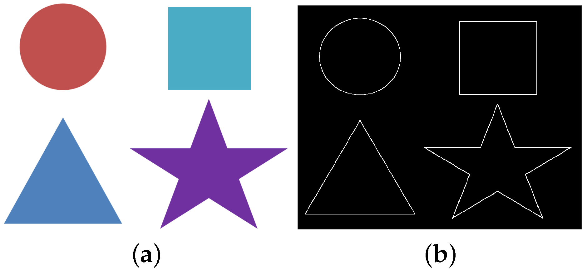
Figure 2.
Used graphical models: (a) the second order Gaussian Markov random field; and (b) circular state space model.
Figure 2.
Used graphical models: (a) the second order Gaussian Markov random field; and (b) circular state space model.

Figure 3.
Comparison of segmentation by three different proposed algorithms for a noise-free image. (a) Detected Points; (b) Detected trajectory via variational Bayes; (c) Segmentation.
Figure 3.
Comparison of segmentation by three different proposed algorithms for a noise-free image. (a) Detected Points; (b) Detected trajectory via variational Bayes; (c) Segmentation.

Figure 4.
Comparison of the segmentation by the three different proposed algorithms for an image with occlusion. (a) Detected points; (b) Detected trajectory via variational Bayes; (c) Segmentation.
Figure 4.
Comparison of the segmentation by the three different proposed algorithms for an image with occlusion. (a) Detected points; (b) Detected trajectory via variational Bayes; (c) Segmentation.
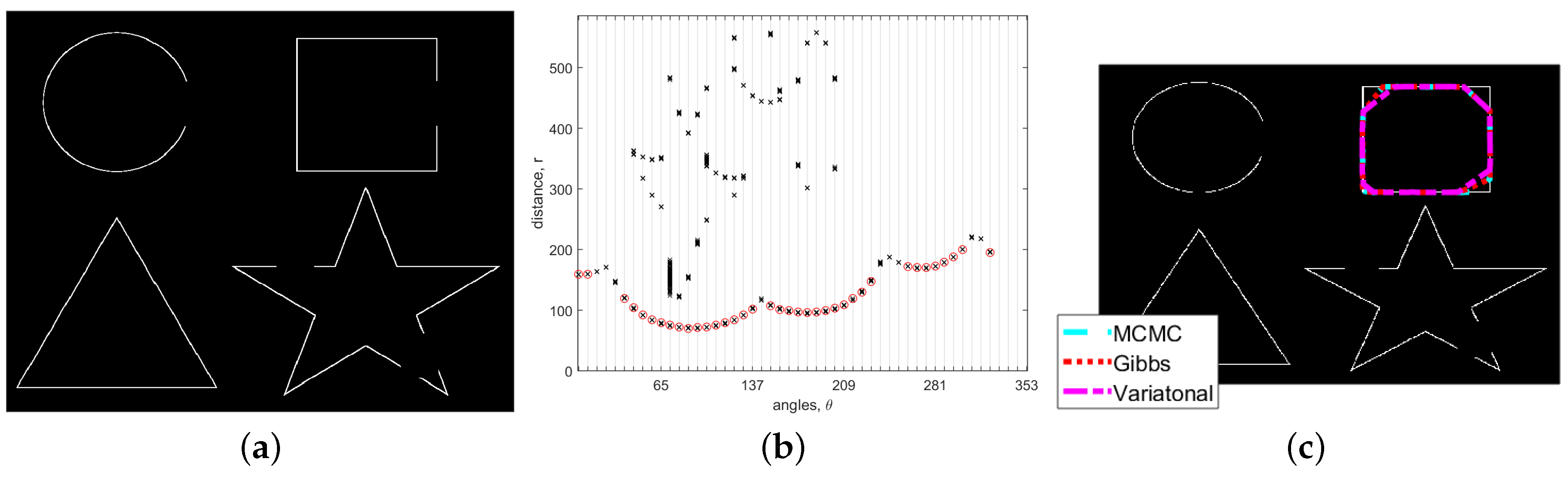
Figure 5.
Raw image, hidden true segmentation for ground truth determination, points detected by the “Sobel” detector and the linked boundaries. (a) Raw image; (b) True segmentation; (c) Detected points; (d) Linked edges.
Figure 5.
Raw image, hidden true segmentation for ground truth determination, points detected by the “Sobel” detector and the linked boundaries. (a) Raw image; (b) True segmentation; (c) Detected points; (d) Linked edges.

Figure 6.
Comparison of edge linking with varying noisy rate, . (a) ; (b) ; (c) ; (d) .


Figure 7.
Interactive segmentation via Canny detection.
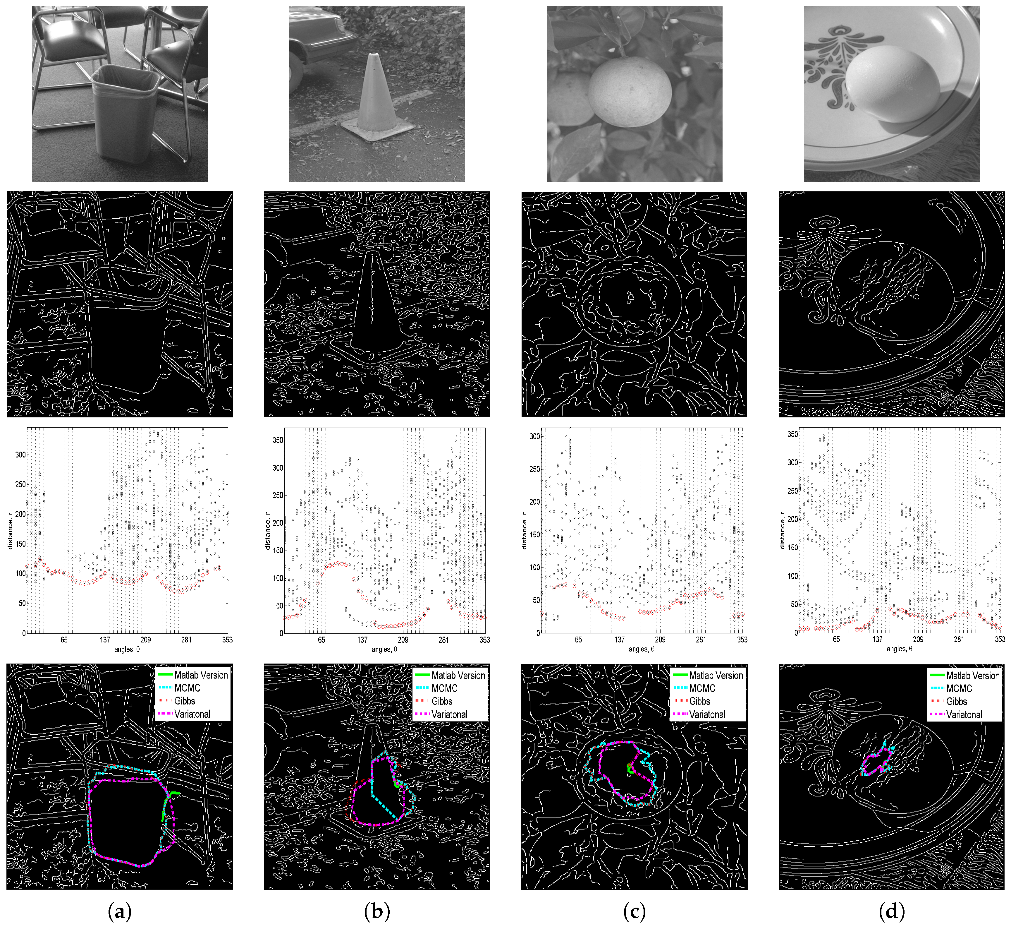
Figure 8.
Interactive segmentation via three different detection algorithms.

| Overlapping Rate (Average ± Std) | ||||
| MATLAB | MCMC | Gibbs | VB | |
| 0 | 0.77 0.10 | |||
| 0.76 0.08 | ||||
| 0.72 0.15 | ||||
| 0.64 0.14 | ||||
| Execution Time (Average ± Std) | ||||
| MATLAB | MCMC | Gibbs | VB | |
| 0 | ||||
| Image | Execution Time | |||
|---|---|---|---|---|
| MATLAB | MCMC | Gibbs | VB | |
| (a) | 1.7519 | 405.45 | 371.02 | 13.751 |
| (b) | 2.1913 | 447.51 | 525.08 | 19.322 |
| (c) | 1.5243 | 355.21 | 434.16 | 9.8595 |
| (d) | 1.7146 | 359.09 | 450.6 | 10.566 |
© 2016 by the author; licensee MDPI, Basel, Switzerland. This article is an open access article distributed under the terms and conditions of the Creative Commons Attribution (CC-BY) license (http://creativecommons.org/licenses/by/4.0/).
Share and Cite
MDPI and ACS Style
Yoon, J.W. A New Bayesian Edge-Linking Algorithm Using Single-Target Tracking Techniques. Symmetry 2016, 8, 143. https://doi.org/10.3390/sym8120143
AMA Style
Yoon JW. A New Bayesian Edge-Linking Algorithm Using Single-Target Tracking Techniques. Symmetry. 2016; 8(12):143. https://doi.org/10.3390/sym8120143
Chicago/Turabian StyleYoon, Ji Won. 2016. "A New Bayesian Edge-Linking Algorithm Using Single-Target Tracking Techniques" Symmetry 8, no. 12: 143. https://doi.org/10.3390/sym8120143
Note that from the first issue of 2016, this journal uses article numbers instead of page numbers. See further details here.