Testing Lorentz Symmetry Using High Energy Astrophysics Observations


1
NASA Goddard Space Flight Center, Greenbelt, MD 20771, USA
2
Department of Physics and Astronomy, University of California, Los Angeles, CA 90095, USA
Symmetry 2017, 9(10), 201; https://doi.org/10.3390/sym9100201
Submission received: 17 August 2017
/
Accepted: 19 September 2017
/
Published: 25 September 2017
(This article belongs to the Special Issue Violation of Lorentz Symmetry)
Abstract
:We discuss some of the tests of Lorentz symmetry made possible by astrophysical observations of ultrahigh energy cosmic rays, -rays and neutrinos. These are among the most sensitive tests of Lorentz invariance violation because they are the highest energy phenomena known to man.
1. Introduction
One of the main motivations for testing Lorentz symmetry comes from the search for an answer to one of the most fundamental problems of modern physics: how to reconcile general relativity with quantum physics. This problem is particularly acute on the length scale where the effect of quantum fluctuations on spacetime cannot be ignored. This scale, known as the Planck length, is given by m [1]. It corresponds to the very large energy scale, GeV, where . (Hereafter, we use the conventions for the low energy speed of light and .) The open question of constructing a framework for a quantum theory of gravity is intimately related to the question of Lorentz invariance violation [2,3].
Lorentz symmetry implies scale-free spacetime. The group of Lorentz transformations is unbounded in energy (boost) space. Owing to the uncertainty principle, the higher the particle energy attained, the smaller the scale of physics that can be probed. Very high energy interactions probe physics at ultra-short distance intervals, . Thus, to probe physics at small distance intervals, particularly the nature of space and time, we need to go to ultrahigh energies. Cosmic -rays and neutrinos and cosmic-ray nucleons provide the highest observable energies in the universe.
This paper reviews the topic of testing the exactness of Lorentz symmetry using astrophysical observations of ultrahigh energy cosmic rays, -rays and neutrinos. (For a review of tests of Lorentz symmetry in the gravitational sector, see [4].) Cosmic -rays have been observed at energies up to GeV. Neutrinos of astrophysical origin have been observed at energies up to GeV. Even ultrahigh energy cosmic ray nuclei have been observed only up to GeV energy. These energies are much lower than . However, the effects of violations of Lorentz invariance (LIV) can be manifested at energies much lower than . (By Noether’s theorem, Lorentz symmetry implies Lorentz invariance; here we use these terms interchangeably.)
There are many ways that LIV terms in the free particle Lagrangian can affect physics at astrophysically-accessible energies. In particular, the effect of LIV can change the kinematics of particle interactions and decays and also the threshold energies for these processes [5,6]. LIV can also modify neutrino oscillations [5,7].
2. The Coleman–Glashow Formalism
As an initial framework for exploring the effects of LIV, we start with the phenomenological approach of Coleman and Glashow [5]. This formalism has the advantage of (1) simplicity, (2) preserving the standard model of strong and electroweak interactions, (3) having the perturbative term in the Lagrangian consist of operators of mass dimension four that thus preserves power counting renormalizability and (4) being rotationally invariant in a preferred frame that can be taken to be the rest frame of the CBR (Cosmic background radiation). Coleman and Glashow start with a standard-model free-particle Lagrangian,
where the matrices are in boldface, is a column vector of n fields with U(1) invariance, and the positive Hermitian matrices , and M can be transformed so that is the identity and M is diagonalized to produce the standard theory of n decoupled free fields. (We adopt the standard notation of denoting four-vector indexes by Greek letters and three-vector spatial indexes by Latin letters).
They then add a leading order perturbative, Lorentz violating term constructed from only spatial derivatives with rotational symmetry so that:
where is a small dimensionless Hermitian matrix that commutes with M so that the fields remain separable and the resulting single particle energy-momentum eigenstates go from eigenstates of M at low energy to eigenstates of at high energies.
To leading order, this term shifts the poles of the propagator, resulting in the free particle dispersion relation:
This can be put in the standard form for the dispersion relation:
by shifting the renormalized mass by the small amount and shifting the velocity from by the amount . The group velocity is given by:
which goes to in the limit of large . Thus, Coleman and Glashow identify to be the maximum attainable velocity of the free particle. Using this formalism, it becomes apparent that, in principle, different particles can have different maximum attainable velocities (MAVs), which can be different from c. Hereafter, we denote the MAV of a particle of type i by and the difference:
3. LIV Modified Kinematics for QED
Using the formalism of [5], we denote maximum attainable velocity (MAV) of a particle of type i by . We further define the difference , and specifically, here, where is the low energy photon velocity. These definitions will be used to discuss the physics implications of cosmic ray and cosmic -ray observations [6].
If , the decay of a photon into an electron-positron pair is kinematically allowed for photons with energies exceeding . This decay would take place rapidly, so that photons with energies exceeding could not be observed either in the laboratory or as cosmic rays. Since photons have been observed with energies 50 TeV from the Crab Nebula [8], this implies that TeV, or that .
If, on the other hand, , electrons become superluminal if their energies exceed . Electrons traveling faster than light will emit light at all frequencies by a process of ’vacuum Čerenkov radiation’. The electrons then would rapidly lose energy until they become subluminal. Because electrons have been seen in the cosmic radiation with energies up to 2 TeV [9], it follows that . A smaller, but more indirect, upper limit on for the case can be obtained from theoretical considerations of -ray emission from the Crab Nebula. Its emission above 0.1 GeV, extending into the TeV range, is thought to be Compton emission of the same relativistic electrons that produce its synchrotron radiation at lower energies [10]. The Compton component, extends to 50 TeV and thus implies the existence of electrons having energies at least this great in order to produce 50 TeV photons, even in the extreme Klein-Nishina limit. This indirect argument, based on the reasonable assumption that the 50-TeV -rays are from Compton interactions, leads to a smaller upper limit on , viz., . A further constraint on for follows from a change in the threshold energy for the pair production process . This follows from the fact that the square of the four-momentum is changed to give the threshold condition:
where is the energy of the low energy photon and is the angle between the two photons. The second term on the left-hand side comes from the fact that . It follows that the condition for a significant increase in the energy threshold for pair production is ≥ , or equivalently,
The -ray spectrum of the active galaxy Mkn 501 while flaring extended to TeV [10] and exhibited the high energy absorption expected from -ray annihilation by extragalactic pair-production interactions with extragalactic infrared photons [11,12,13]. This has led Stecker and Glashow [6] to point out that the Mkn 501 spectrum presents evidence for pair-production with no indication of Lorentz invariance violation (LIV) up to a photon energy of ∼20 TeV and to thereby place a quantitative constraint on LIV given by . This constraint on positive is more secure than the smaller, but indirect, limit given above. See [14] for further considerations regarding the modification of -ray spectra by LIV.
4. Ultrahigh Energy Cosmic Rays
4.1. Extragalactic Origin
Ultrahigh energy cosmic rays (UHECRs) appear to have an isotropic distribution in arrival direction. Because of their ultrahigh energy, their propagation is little affected by galactic magnetic fields. Thus, owing to their observed isotropy, cosmic rays above 10 EeV ( eV) are believed to be of extragalactic origin.
4.2. The Greisen–Zatsepin–Kuz’min Effect
Shortly after the discovery of the 2.7 K CBR, Greisen [15] and Zatsepin and Kuz’min [16] predicted that pion-producing interactions of UHECR protons with the microwave photons of the CBR should produce a spectral cutoff at 50 EeV. The flux of UHECRs is thus expected to be attenuated by such meson-producing interactions. This effect is generally known as the “GZK (Greisen–Zatsepin–Kuz’min) effect”. Owing to these interactions, extragalactic protons with energies above ∼100 EeV should be attenuated while propagating from distances beyond ∼100 Mpc [17]. The cross-section for this process peaks at the baryon resonance,
The energy threshold for photomeson interactions of UHECR protons of initial laboratory energy E with low energy photons of the 2.7 blackbody CBR having laboratory energy is determined by the relativistic invariance of the square of the total four-momentum of the proton-photon system. This relation, together with the threshold inelasticity relation for single pion production, yields the threshold conditions for head on collisions in the laboratory frame:
for the proton, and:
for the pion, where M is the rest mass of the proton and m is the rest mass of the pion [17].
5. Modification of the GZK Effect
We have previously discussed the observations of UHECRs and their expected attenuation over extragalactic distances owing to the GZK effect. We now turn our attention to how the GZK effect can be modified by a very small violation of Lorentz symmetry.
5.1. Energy Threshold
If Lorentz symmetry is slightly broken so that , it follows from Equations (6), (11) and (22) and that the threshold energy for photomeson is altered because the square of the four-momentum is shifted from its LI form so that the threshold condition in terms of the pion energy becomes:
Equation (12) is a quadratic equation with real roots only under the condition:
Defining eV with K, Equation (13) can be rewritten:
Equation (14) implies that if Lorentz symmetry is violated and for , photomeson interactions with CBR photons will not occur for . This condition, together with Equation (12), implies that while photomeson interactions leading to GZK suppression can occur for “lower energy” UHE protons interacting with higher energy CBR photons on the Wien tail of the CBR blackbody spectrum, other interactions involving higher energy protons and photons with smaller values of will be forbidden. Thus, the observed UHECR spectrum may exhibit the characteristics of GZK suppression near the normal GZK threshold, but the UHECR spectrum can “recover” at higher energies owing to the possibility that photomeson interactions at higher proton energies may be forbidden.
5.2. Detailed GZK Kinematics with LIV
We have seen that kinematical relations governing photomeson interactions are changed in the presence of even a small violation of Lorentz invariance. We now consider this in more detail [18].
Following Equations (6) and (22), we denote:
where is the difference between the MAV for the particle a and the speed of light in the low momentum limit ().
In the cms (center-of-momentum system), the energy of particle a is then given by:
Owing to LIV, in the cms, the particle will not generally be at rest when because:
The modified kinematical relations containing LIV have a strong effect on the amount of energy transferred from an incoming proton to the pion produced in the subsequent interaction, i.e., the inelasticity [18,19]. The total inelasticity, K, is an average of , which depends on the angle between the proton and photon momenta, :
The primary effect of LIV on photopion production is a reduction of phase space allowed for the interaction. This results from the limits on the allowed range of interaction angles integrated over in order to obtain the total inelasticity from Equation (18). For real-root solutions for interactions involving higher energy protons, the range of kinematically allowed angles in Equation (18) becomes severely restricted. The modified inelasticity that results is the key in determining the effects of LIV on photopion production. The inelasticity rapidly drops for higher incident proton energies.
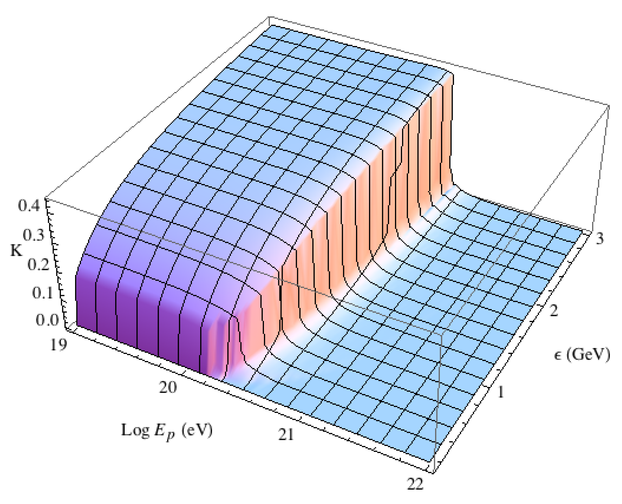
Figure 1 shows the calculated proton inelasticity modified by LIV for a value of as a function of both CBR photon energy and proton energy [18]. Other choices for yield similar plots. The principal result of changing the value of is to change the energy at which LIV effects become significant. For a choice of , there is no observable effect from LIV for less than EeV. Above this energy, the inelasticity precipitously drops as the LIV term in the pion rest energy approaches .
With this modified inelasticity, the proton energy loss rate by photomeson production is given by:
where is the photon threshold energy for the interaction and is the total -p cross-section with contributions from direct pion production, multipion production and the resonance.
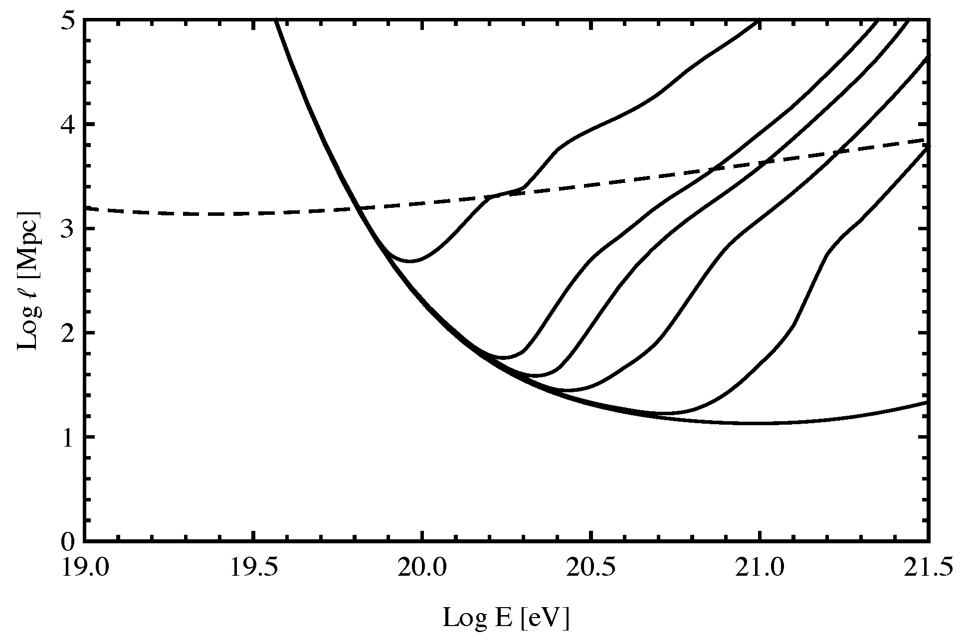
The corresponding proton attenuation length is given by , where the energy loss rate . This attenuation length is plotted in Figure 2 for various values of along with the unmodified pair production attenuation length from pair production interactions, .
6. Comparison of LIV-Modified UHECR Spectra with Observations
An analytic calculation of LIV-modified UHECR proton spectra was obtained using Equation (19) [18] (see also [19]). In order to take account of the probable redshift evolution of UHECR production in astronomical sources, one must take account of the following considerations [18]:
- The CBR photon number density increases as , and the CBR photon energies increase linearly with . The corresponding energy loss for protons at any redshift z is thus given by:
- It is assumed that the average UHECR volume emissivity is of the form given by where is the initial energy of the proton at the source and . The source evolution is assumed to be with so that is roughly proportional to the empirically-determined z-dependence of the star formation rate. and are normalized to fit the data below the GZK threshold.
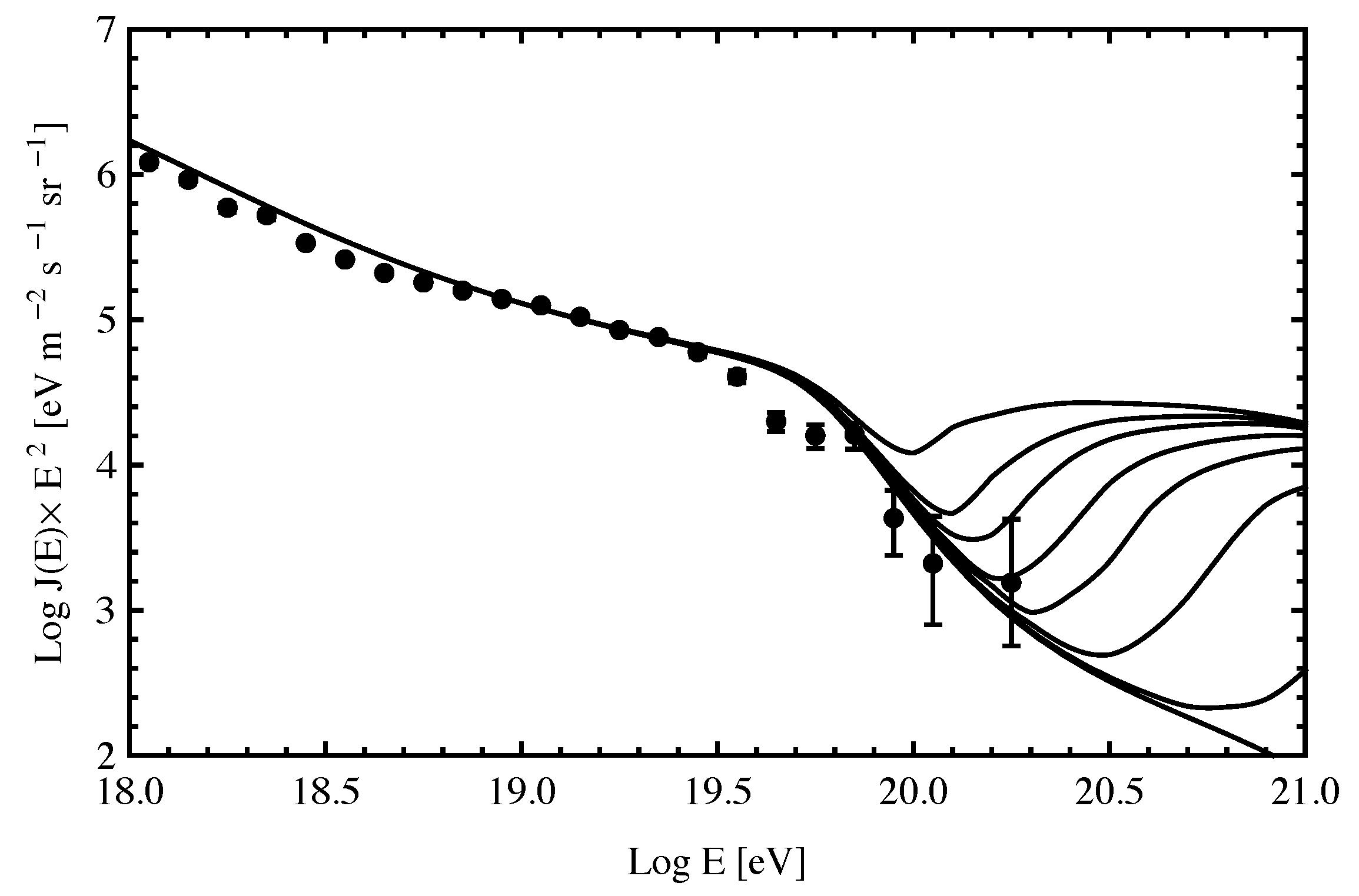
The curves calculated in [18] assuming various values of are shown in Figure 3 along with the Auger data from [20]. They show that even a very small amount of LIV that is consistent with both a GZK effect and with the present UHECR data can lead to a “recovery” of the UHECR spectrum at higher energies.
7. Modified GZK Neutrino Spectrum from a Modified UHECR Spectrum
Subsequent to the photopion interactions of Equation (9), the charged pions that are produced decay to produce neutrinos. It follows from the modified kinematics and inelasticity for photopion interactions as presented in Section 5 (see Figure 1) that there will be a modification of the spectrum of the “GZK neutrinos” that result.
Figure 4 shows the corresponding total neutrino flux (all species) for the same choices of as the UHECR spectra presented in Figure 3. As expected, increasing leads to a decreased flux of higher energy photomeson neutrinos because the interactions involving higher energy UHECRs are suppressed [21]. It is also evident that the peak energy of the neutrino energy flux spectrum (EFS), , shifts to lower energies with increasing .
This possible LIV effect on GZK neutrinos may be tested using radio arrays built on Antarctic ice that are based on the Askaryan effect such as the Askaryan Radio Array (ARA) [22] and the Antarctic Ross Ice-Shelf Antenna Neutrino Array (ARIANNA) [23]. GZK effect neutrinos can also be observed by space-based telescopes looking down at the atmosphere to study the horizontal air showers they produce [24,25].
8. Generalizing the Coleman–Glashow Formalism
The Coleman–Glashow formalism preserves a renormalizable Lagrangian structure, with the Lagrangian density being of mass-dimension . More generally, it is possible to construct an extended standard model (SME) Lagrangian as an effective field theory formalism that is testable and that holds at energies [2]. This formalism admits LIV terms composed of operators of dimension suppressed by values of . It is motivated by two ideas: (1) any LIV extant at accelerator energies must be extremely small and (2) physics must be strongly modified at the Planck energy, . These considerations are reflected by adding small Lorentz-violating terms in the free particle Lagrangian that are suppressed by powers of some quantum gravity energy scale ∼. Sums of such terms are also possible and, as such, admit energy-dependent values of ,
where we will consider only terms up to n = 2. In the SME formalism, the n = 1 term corresponds to the lowest order -odd operator, and the n = 2 term corresponds to the lowest order -even operator. We now consider two applications of this formalism.
8.1. Time of Flight from -ray Bursts
Energy-dependent MAVs constructed by assuming that LIV is related to physics at the Planck scale have been used in time-of-flight observations of photon arrival times from cosmologically-distant -ray bursts. For this analysis, LIV modifications to the photon dispersion relation were taken to be the sum of a series of terms in [26],
where it was expected that = . In Equation (22), is the “sign of LIV”, taken equal to +1 (−1) for a decrease (increase) in photon MAV with an increasing photon energy. In case the term is suppressed, owing to conservation of , the is assumed to dominate.
Adopting the notation of [27], we define an“LIV parameter” as the ratio of the time delay between photons of the highest observed energy, , and the lowest observed energy, , and the quantity − . Then:
where:
where is a cosmological distance parameter. (Values of are conventionally defined as fractions of the critical density needed to close the universe, .) Here, as usual, z is redshift; is the Hubble constant; and values of and are designated for the dark energy density and total matter density, respectively. The Hubble constant is taken to be 67.8 km s Mpc; = 0.7; and = 0.3.
Three different statistical analyses on Fermi observations of three -ray bursts have been used to derive strong constraints on [27]. The most stringent limits for at the 95% confidence level are obtained from the -ray burst GRB 090510 and are and GeV for linear and quadratic leading order LIV-induced vacuum dispersion, respectively.
An early suggestion for testing quantum gravity [28] employed the natural idea of identifying . A later “D-brane” model, inspired by string theory concepts, suggested the prospect that only photons would exhibit an energy-dependent velocity [29]. That model envisions a universe filled with a gas of point-like D-branes that only interact with photons. It predicts that vacuum has an energy-dependent index of refraction that causes only a retardation, again with . Such models are disfavored by the analysis of the Fermi observations that, on its face, appears to suggest .
8.2. Gamma-Ray Absorption with Planck Suppressed LIV
Motivated by the time-of-flight result above, we drop the condition from Equation (22) that and consider . Using Equation (21), the energy threshold for relation (8) is modified slightly in the Planck-suppressed LIV case. If we again take the condition for LIV to significantly change the threshold energy for absorption as given by the relation (8), with given by Equation (21), the criterion for an absorption feature in the -ray energy spectrum of a source to be affected by an LIV term with Planck suppression becomes:
where n is the lowest value for the LIV term that dominates in the series (21). The case was first treated in [30]. This topic has been considered further in [14].
9. Vacuum Birefringence
Important fundamental constraints on LIV come from searches for the vacuum birefringence effect predicted within the framework of the effective field theory (EFT) analysis of [31] (see also [32,33]). Within this framework, applying the Bianchi identities to the leading order Maxwell equations in vacuo, a -odd mass dimension five operator term is derived of the form:
It is shown in [31] that the expression given in Equation (27) is the only dimension five modification of the free photon Lagrangian that preserves both rotational symmetry and gauge invariance. This leads to a modification in the dispersion relation proportional to , with the new dispersion relation given by:
with photons of opposite helicity having slightly different velocities. This leads to a rotation in the angle of polarization,
for a plane wave with wave-vector k, where and where is the propagation time.
Observations of polarized radiation from distant sources can thus be used to place an upper bound on . The vacuum birefringence constraint arises from the fact that if the angle of polarization rotation (29) were to differ by more than over the energy range covered by the observation, the instantaneous polarization at the detector would fluctuate sufficiently for the net polarization of the signal to be suppressed well below any observed value. The difference in rotation angles for wave-vectors and is:
where we have replaced the propagation time by the propagation distance from the source to the detector.
If polarization is detected from a source at redshift z, this yields the constraint:
where and:
10. LIV in the Neutrino Sector
There are many ways that LIV terms in the free particle Lagrangian can affect neutrino physics. We will here consider only one of these consequences, viz., the effect of resulting changes in the kinematics of particle interactions. (A discussion of the effect of LIV on modifying neutrino oscillations may be found in [7].) These changes can modify the threshold energies for particle interactions, allowing or forbidding such interactions [5,6]. Observational evidence for this effect can be searched for by examining the energy spectrum of high energy cosmic neutrinos obtained by the IceCube collaboration. We base our discussion of this evidence on the well delineated framework of the standard model extension (SME) formalism of effective field theory (EFT) [32], as given in more detail in [36].
10.1. Fermion LIV Operators with LIV with Rotational Symmetry in SME
We again assume rotational invariance in the rest frame of the CBR and consider only the effects of Lorentz violation on freely-propagating cosmic neutrinos. Thus, we only need to examine Lorentz-violating modifications to the neutrino kinetic terms. Majorana neutrino couplings are ruled out in SME in the case of rotational symmetry [37]. Therefore, we only consider Dirac neutrinos.
Using Equation (22), one can define an effective mass, , that is a useful parameter for analyzing LIV-modified kinematics. The effective mass is constructed to include the effect of the LIV terms. We define an effective mass for a particle for type I using the dispersion relation (22) as [5,36]:
where the velocity parameters are now energy-dependent dimensionless coefficients for each species, I, that are contained in the Lagrangian. Furthermore, we define the parameter as the Lorentz-violating difference between the MAVs of particles I and J. In general, will therefore be of the form given by Equation (21).
If we wish to assume the dominance of Planck-suppressed terms in the Lagrangian as tracers of Planck-scale physics, it follows that that . (Several mechanisms have been proposed for the suppression of the LIV term in the Lagrangian. See, e.g., the review in Reference [38].) Alternatively, we may postulate the existence of only Planck-suppressed terms in the Lagrangian, i.e., . We can further simplify by noting the important connection between LIV and violation. Whereas a local interacting theory that violates invariance will also violate Lorentz invariance [39], the converse does not follow; an interacting theory that violates Lorentz invariance may, or may not, violate invariance. LIV terms of odd mass dimension are -odd and violate , whereas terms of even mass dimension are -even and do not violate [40].
We can then specify a dominant term for in Equation (21) depending on our choice of . Considering Planck-mass suppression, the dominant term that admits violation is the term in Equation (21). On the other hand, if we require conservation, the term in Equation (21) is the dominant term. Thus, we can choose as a good approximation to Equation (21), a single dominant term with one particular power of n by specifying whether we are considering -even or odd LIV. As a result, reduces to Equation (21) with or depending on the status of . We note that in the SME formalism, since -odd LIV operators are -odd, the -conjugation property implies that neutrinos can be superluminal, while antineutrinos are subluminal or vice versa [37]. This will have consequences in interpreting our results, as we will discuss later.
In Equations (21) and (22), we have not designated a helicity index on the coefficients. The fundamental parameters in the Lagrangian are generally helicity dependent. In the case, a helicity dependence must be generated in the electron sector due to the -odd nature of the LIV term. However, the constraints on the electron coefficient are extremely tight from observations of the Crab Nebula [41]. Thus, the contribution to from the electron sector can be neglected. In the case, which is -even, we can set the left- and right-handed electron coefficients to be equal by imposing parity symmetry [36].
10.2. LIV in the Neutrino Sector I: Lepton Pair Emission
Since the Lorentz violating operators change the free field behavior and dispersion relation, interactions such as fermion-antifermion pair emission by slightly superluminal neutrinos become kinematically allowed [5,42] and can thus cause significant observational effects. An example of such an interaction is “splitting”, i.e., where i is a flavor index. Neutrino splitting can be represented as a rotation of the Feynman diagram for neutrino-neutrino scattering, which is allowed by relativity. However, absent a violation of Lorentz invariance, neutrino splitting is forbidden by conservation of energy and momentum. In the the case of LIV-allowed superluminal neutrinos, the dominant pair emission reactions are neutrino splitting and its close cousin, vacuum electron-positron pair emission (VPE) , as these are the reactions with the lightest final state masses. We now set up a simplified formalism to calculate the possible observational effect of these two specific anomalous interactions on the interpretation of the neutrino spectrum observed by the IceCube collaboration.
10.2.1. Lepton Pair Emission in the [d] = 4 Case
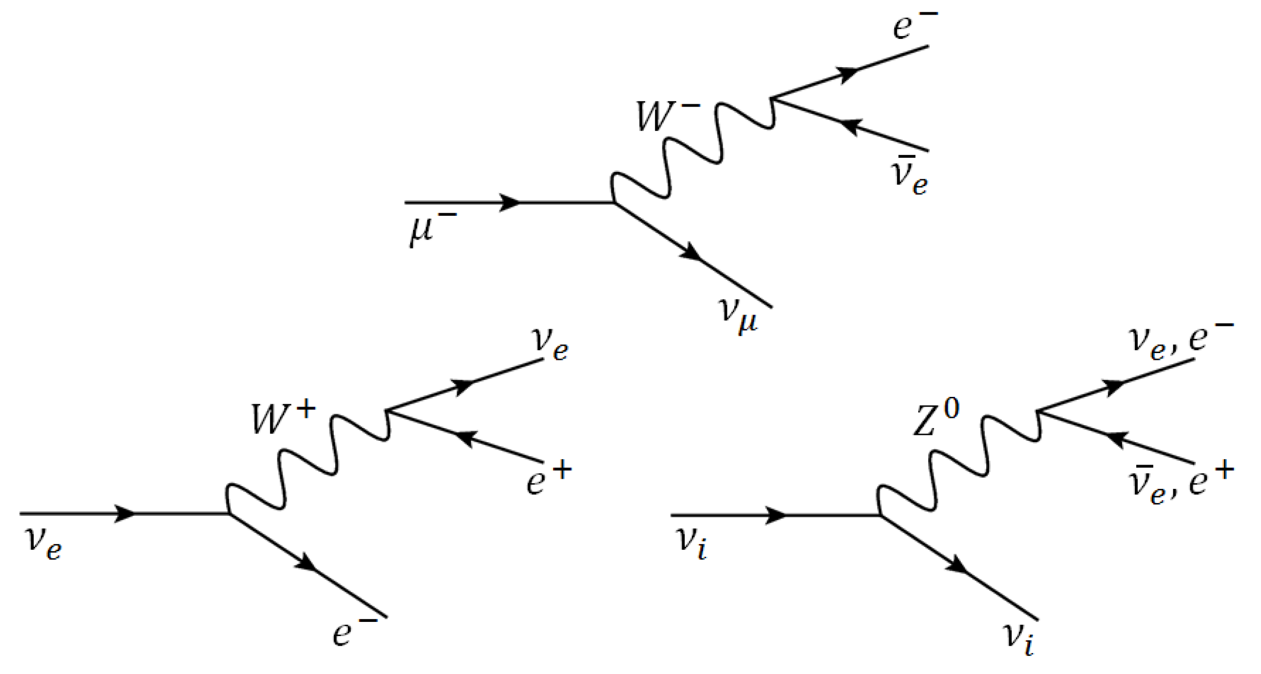
In this section, we consider the constraints on the LIV parameter . We first relate the rates for superluminal neutrinos with that of a more familiar tree level, weak force-mediated standard model decay process: muon decay, , as the processes are very similar (see Figure 5).
For muons with a Lorentz factor in the observer’s frame, the decay rate is found to be:
where is the square of the Fermi constant equal to , with g being the weak coupling constant and being the W-boson mass in electroweak theory.
We apply the effective energy-dependent mass-squared formalism given by Equation (33) to determine the scaling of the emission rate with the parameter and with energy. Noting that for any reasonable neutrino mass, , it follows that . (At relativistic energies, assuming that the Lorentz violating terms yield small corrections to E and p, it follows that .)
We therefore make the substitution:
from which it follows that:
The rate for the vacuum pair emission processes (VPE) is then:
which gives the proportionality:
showing the strong dependence of the decay rate on both and .
The energy threshold for pair production is given by [6]:
with given by Equation (21), the rate for the VPE process, , via the neutral current Z-exchange channel, has been calculated to be [42]:
with the mean fractional energy loss per interaction from VPE of 78% [42].
In general, the charged current (CC) W-exchange channels contribute as well. However, this channel is only kinematically relevant for ’s, as the production of or leptons by ’s or ’s has a much higher energy threshold due to the larger final state particle masses (Equation (39) with replaced by or ), with the neutrino energy loss from VPE being highly threshold dependent. Owing to neutrino oscillations, neutrinos propagating over large distances spend 1/3 of their time in each flavor state. Thus, the flavor population of neutrinos from astrophysical sources is expected to be [::] = [1:1:1] so that CC interactions involving ’s will only be important 1/3 of the time.
The vacuum Čerenkov emission (VCE) process, , is also kinematically allowed for superluminal neutrinos. However, since the neutrino has no charge, this process entails the neutral current channel production of a loop consisting of a virtual electron-positron pair followed by its annihilation into a photon. Thus, the rate for VCE is a factor of lower than that for VPE.
10.2.2. Vacuum Pair Emission in the Cases
Using Equations (21) and (38) and the dynamical matrix element taken from the simplest case [43], we can generalize Equation (40) for arbitrary values of [36].
where is the sine of the Weinberg angle () and the ’s are numbers of order 1 [43].
For the case, we obtain the VPE rate:
and for the case, we obtain the VPE rate:
11. LIV in the Neutrino Sector II: Neutrino Splitting
The process of neutrino splitting in the case of superluminal neutrinos, i.e., , is relatively unimportant in the case [42] owing to the small velocity difference between neutrino flavors obtained from neutrino oscillation data [44,45,46]. However, this is not true in the cases with . In the presence of terms in a Planck-mass suppressed EFT, the velocity differences between the neutrinos, being energy dependent, become significant [47]. The daughter neutrinos travel with a smaller velocity. The velocity-dependent energy of the parent neutrino is therefore greater than that of the daughter neutrinos. Thus, the neutrino splitting becomes kinematically allowed. Let us then consider the and scenarios.
Neutrino splitting is a neutral current (NC) interaction that can occur for all three neutrino flavors. The total neutrino splitting rate obtained is therefore three times that of the NC-mediated VPE process above threshold. Assuming the three daughter neutrinos each carry off approximately 1/3 of the energy of the incoming neutrino, then for the case, one obtains the neutrino splitting rate [36]:
and for the case, we obtain the neutrino splitting rate:
The threshold energy for neutrino splitting is proportional to the neutrino mass so that it is negligible compared to that given by Equation (39).
12. The Neutrinos Observed by IceCube
As of this writing, the IceCube collaboration has identified events from neutrinos of astrophysical origin with energies above 10 TeV, with the error in the number of astrophysical events determined by the modeled subtraction of both conventional and prompt atmospheric neutrinos and also penetrating atmospheric muons at energies below 60 TeV [48].
There are are four indications that the bulk of cosmic neutrinos observed by IceCube with energies above 0.1 PeV are of extragalactic origin: (1) the arrival distribution of the reported events with PeV observed by IceCube above atmospheric background is consistent with isotropy [48,49,50]; (2) at least one of the PeV neutrinos came from a direction off the galactic plane [48]; (3) the diffuse galactic neutrino flux is expected to be well below that observed by IceCube [51]; (4) upper limits on diffuse galactic -rays in the TeV–PeV energy range imply that galactic neutrinos cannot account for the neutrino flux observed by IceCube [52].
Above 60 TeV, the IceCube data are roughly consistent with a spectrum given by [48,49,50]. However, IceCube has not detected any neutrino-induced events from the Glashow resonance effect at PeV [53]. At the Glashow resonance energy electrons in the IceCube volume provide enhanced target cross-sections for ’s through the resonance channel, . This enhancement effect is expected to be about a factor of ∼10 [50]. Owing to oscillations, it is expected that 1/3 of the potential 6.3 PeV neutrinos would be ’s plus ’s unless new physics is involved.
Thus, the enhancement in the overall effective area expected is a factor of ∼3. Taking account of the increased effective area between 2 and 6 PeV and a decrease from an assumed neutrino energy spectrum of , we would expect about three events at the Glashow resonance energy, provided that the number of ’s is equal to the number of ’s. Even without considering the resonance effect, several neutrino events above 2 PeV would be expected if the spectrum extended to higher energies. Thus, the lack of this flux of neutrinos above ∼2 PeV energy and at the 6.3-PeV resonance may be indications of a cutoff in the neutrino spectrum. (Since [36] was published, an event with a deposited energy of 2.6 PeV was reported by the IceCube collaboration. The energy of the neutrino that produced this event may have been as high as 6 PeV, although this is uncertain [54].)
13. Extragalactic Superluminal Neutrino Propagation
Monte Carlo techniques have been employed to determine the effect of neutrino splitting and VPE on putative superluminal neutrinos [36,41]. Extragalactic neutrinos were propagated from cosmological distances taking account of the resulting energy loss effects by VPE and redshifting in the case. In the cases, energy loses include those from both neutrino splitting and VPE, as well as redshifting. It was assumed that the neutrino sources have a redshift distribution similar to that of the star formation rate [55]. Such a redshift distribution appears to be roughly applicable for both active galactic nuclei and -ray bursts. A simple neutrino source spectrum proportional to ∼ was assumed between 100 TeV and 100 PeV, as is the case for cosmic neutrinos observed by IceCube with energies above 60 TeV [49]. The final results on the propagated spectrum were normalized to an energy flux of , consistent with the IceCube data for both the Southern and Northern Hemisphere. Results were obtained for VPE threshold energies between 10 PeV and 40 PeV as given by Equation (39), corresponding to values of between .
Since the neutrinos are extragalactic and survive propagation from all redshifts, cosmological effects must be taken into account in deriving new LIV constraints. Most of the cosmic PeV neutrinos will come from sources at redshifts between ∼0.5 and ∼2 [55]. The effect of the cosmological CDM redshift-distance relation is given by:
The energy loss due to redshifting is given by:
14. The Theoretical Neutrino Energy Spectrum
14.1. [d] = 4 Conserving Operator Dominance
In their seminal paper, using Equation (40), Cohen and Glashow [42] showed how the VPE process in the case implied powerful constraints on LIV. They obtained an upper limit of based on the initial observation of high energy neutrinos by IceCube. Further predictions of limits on with cosmological factors taken into account were then made, with the predicted spectra showing a pileup followed by a cutoff [56]. An upper limit of was obtained [57] based on later IceCube observations [50].
Using the energy loss rate given by Equation (40), a value for was obtained based on a model of the redshift evolution of neutrino sources and using Monte Carlo techniques to take account of propagation effects as discussed in Section 13 [36,41]. The upper limit on is given by [41]. Taking this into account, one gets the constraint . The spectra derived therein for the case also showed a pileup followed by a cutoff. The predicted cutoff is determined by redshifting the threshold energy effect.
14.2. [d] = 6 Conserving Operator Dominance
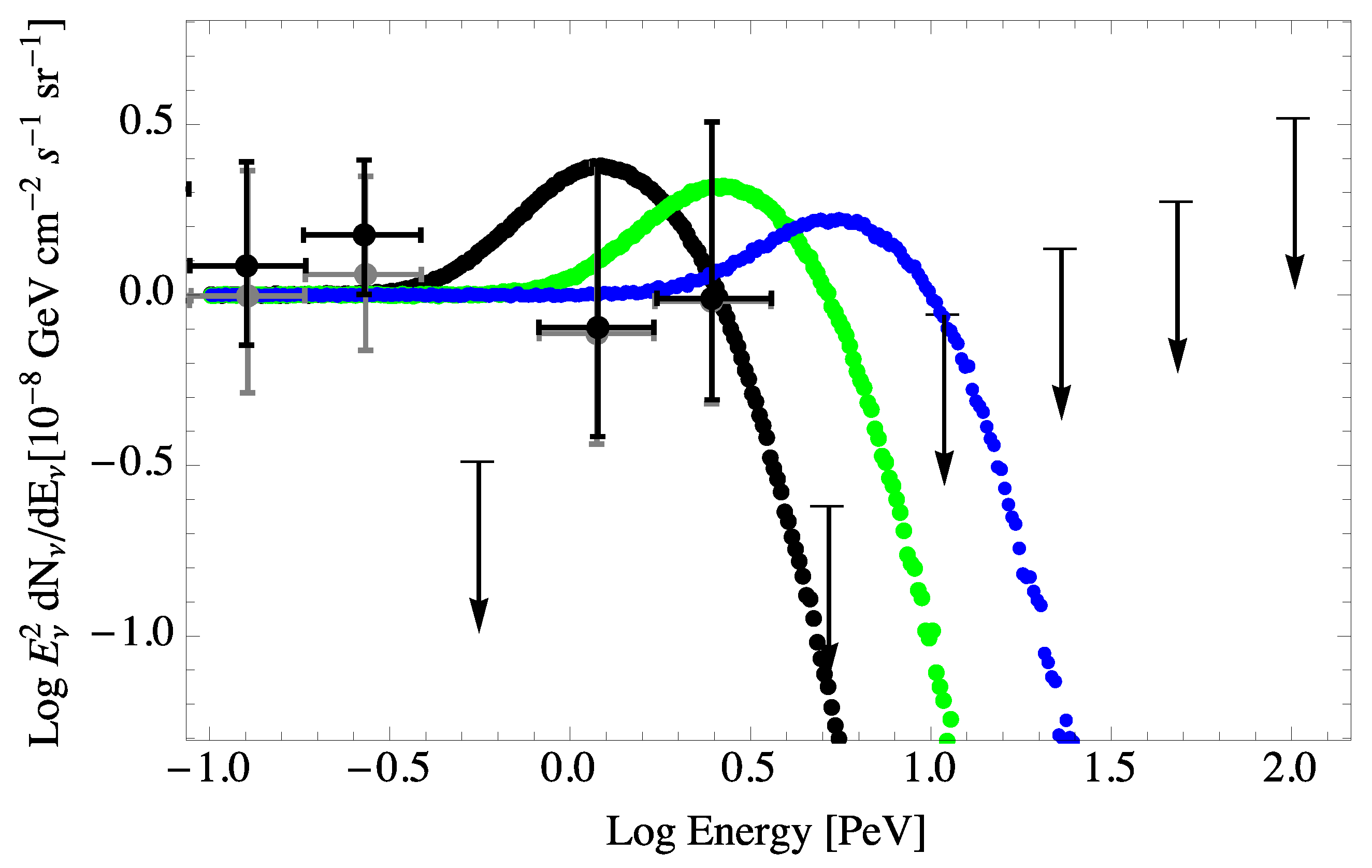
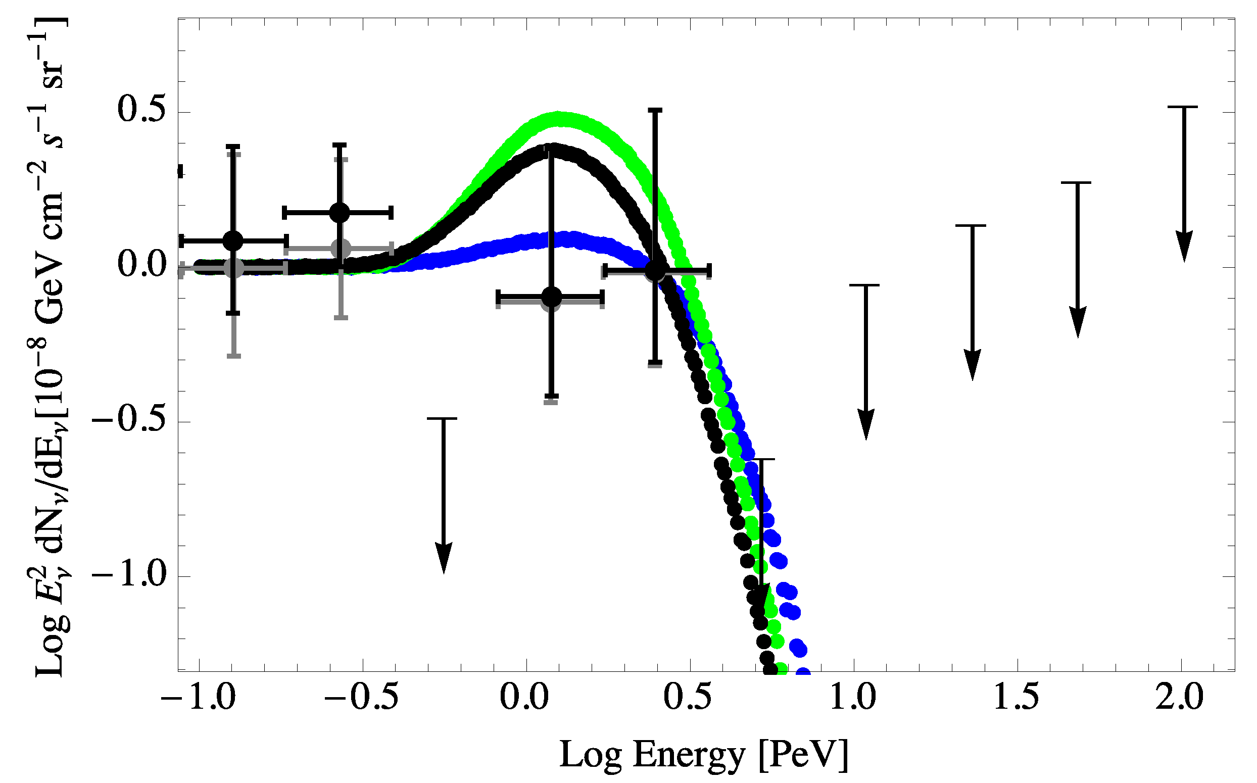
In both the and cases, the best fit matching the theoretical propagated neutrino spectrum, normalized to an energy flux of below 0.3 PeV, with the IceCube data corresponds to a VPE rest-frame threshold energy PeV, as shown in Figure 6 [36,41]. This corresponds to . Given that , it is again found that . As shown in Figure 7, values of less than 10 PeV are inconsistent with the IceCube data. The result for a 10-PeV rest-frame threshold energy is just consistent with the IceCube results, giving a cutoff effect above 2 PeV.
In the case of the conserving operator (n = 2) dominance, as in the case, the results shown in Figure 6 show a high-energy drop off in the propagated neutrino spectrum near the redshifted VPE threshold energy and a pileup in the spectrum below that energy. This predicted drop off may be a possible explanation for the lack of observed neutrinos above 2 PeV [36,41]. This pileup is caused by the propagation of the higher energy neutrinos in energy space down to energies within a factor of ∼5 below the VPE threshold.
The pileup effect caused by the neutrino-splitting process is more pronounced than that caused by the VPE process because neutrino splitting produces two new lower energy neutrinos per interaction. This would be a potential way of distinguishing a dominance of Planck-mass suppressed interactions from interactions. Thus, with better statistics in the energy range above 100 TeV, a significant pileup effect would be a signal of Planck-scale physics. Pileup features are indicative of the fact that fractional energy loss from the last allowed neutrino decay before the VPE process ceases is 78% [42], and that for neutrino splitting is taken to be 1/3. The pileup effect is similar to that of energy propagation for ultrahigh energy protons near the GZK threshold [58].
14.3. [d] = 5 CPT Violating Operator Dominance
In the n = 1 case, the dominant operator violates . Thus, if the is superluminal, the will be subluminal, and vice versa. However, the IceCube detector cannot distinguish neutrinos from antineutrinos. The incoming ) generates a shower in the detector, allowing a measurement of its energy and direction. Even in cases where there is a muon track, the charge of the muon is not determined.
There would be an exception for electron antineutrinos at 6.3 PeV, given an expected enhancement in the event rate at the Glashow resonance since this resonance only occurs with . We note that oscillation measurements would give the strongest constraints on the difference in ’s between ’s and ’s [45].
Since both VPE and neutrino-splitting interactions generate a particle-antiparticle lepton pair, one of the pair particles will be superluminal (), whereas the other particle will be subluminal () [33]. Thus, of the daughter particles, one will be superluminal and interact, while the other will only redshift. The overall result in the case is that no clear spectral cutoff occurs [36].
15. Summary: Results for Superluminal Neutrinos
In the SME EFT formalism [2,32,33], if the apparent cutoff above PeV in the neutrino spectrum shown in Figure 7 is caused by LIV, this would result from an EFT with either a dominant term with , or by a dominant term with GeV [36]. Such a cutoff would not occur if the dominant LIV term is a -violating the operator (However, see [54].) An event with energy significantly above 3 PeV would increase our constraints by as much as an order of magnitude. However, there is still the lack of expected Glashow resonance events to consider.
If the lack of neutrinos at the Glashow resonance is the result of LIV effects as shown in Figure 6 and Figure 7, this would imply that there will be no cosmogenic [59,60] ultrahigh energy neutrinos. A less drastic effect in the cosmogenic neutrino spectrum can be caused by a violation of LIV in the hadronic sector at the level of [21].
A cutoff can naturally occur if it is produced by a maximum acceleration energy in the sources. In that case, the parameters given above would be reduced to upper limits. However, the detection of a pronounced pileup just below the cutoff would be prima facie evidence of a -even LIV effect, possibly related to Planck-scale physics. In fact, -even LIV in the gravitational sector at energies below the Planck energy has been considered in the context of Hořava–Lifshitz gravity [61,62].
16. Stable Pions from LIV
Almost all neutrinos are produced by pion decay. It has been suggested that if LIV effects can prevent the decay of charged pions above a threshold energy, thereby eliminating higher energy neutrinos at the Glashow resonance energy and above [63,64]. In order for the pion to be stable above a critical energy , we require that its effective mass as given by Equation (33) is less than the effective mass of the muon that it would decay to, i.e., . This situation requires the condition that [5]. Then, neglecting the neutrino mass, this critical energy energy is given by:
noting that if, as before, we write ; then, for small , it follows that . In terms of SME formalism with Planck-mass suppressed terms, is given by Equation (21) or Equation (21). For example, if we set = 6 PeV, in order to just avoid the Glashow resonance, we get the requirement, .
If a lack of multi-PeV neutrinos is caused by this effect, there will be no pileup below the cutoff energy as opposed to the superluminal cases previously discussed. This would make the stable pion case difficult to distinguish from a natural cutoff caused by maximum cosmic-ray acceleration energies in the neutrino sources.
17. Conclusions
One of the most profound problems of modern physics is how to reconcile general relativity with quantum physics. A unification of these fundamental principles must somehow occur at the Planck scale. While direct observational evidence on the physics at the Planck scale itself is unattainable, within the EFT framework, clues to “quantum gravity” phenomena can be searched for at energies much lower than . One of these clues may be a tiny violation of Lorentz symmetry that may increase with energy. In this regard, it has been recognized that since cosmic -rays and neutrinos and cosmic-ray nucleons provide the highest observable energies in the universe, high energy astrophysics observations can play an important role in searching for clues to Planck-scale physics.
As discussed in this paper, such astrophysical searches have only thus far yielded strong constraints on LIV, verifying the strength of Lorentz symmetry. However, there may be a hint at possible Lorentz symmetry breaking at the level of in the neutrino sector at PeV energies. Better statistics are needed to explore this possibility further.
Acknowledgments
I thank my collaborators in much of the work discussed here: Stefano Liberati, David Mattingly and Sean Scully.
Conflicts of Interest
The authors declare no conflict of interest.
References
- Planck, M. The Theory of Radiation; Dover Publications: New York, NY, USA, 1959; (Translated from 1906). [Google Scholar]
- Kostelecký, V.A.; Samuel, S. Spontaneous breaking of Lorentz symmetry in string theory. Phys. Rev. D 1989, 39, 683–685. [Google Scholar] [CrossRef]
- Tasson, J.D. What do we know about Lorentz invariance? Rpt. Prog. Phys. 2014, 77, 062901. [Google Scholar] [CrossRef] [PubMed]
- Hees, A.; Bailey, Q.G.; Bourgoin, A.; Pihan-Le Bars, H.; Guerlin, C.; Le Poncin-Lafitte, C. Tests of Lorentz Symmetry in the Gravitational Sector. Universe 2016, 2, 30. [Google Scholar] [CrossRef]
- Coleman, S.R.; Glashow, S.L. High-energy tests of Lorentz invariance. Phys. Rev. D 1999, 59, 116008. [Google Scholar] [CrossRef]
- Stecker, F.W.; Glashow, S.L. New tests of Lorentz invariance following from observations of the highest energy cosmic γ-rays. Astropart. Phys. 2001, 16, 97–99. [Google Scholar] [CrossRef]
- Stecker, F.W. Search for the footprints of new physics with laboratory and cosmic neutrinos. Mod. Phys. Lett. A 2017, 32. [Google Scholar] [CrossRef]
- Tanimori, T.; Sakurazawa, K.; Dazeley, S.A.; Edwards, P.G.; Hara, T.; Hayami, Y.; Kamei, S.; Kifune, T.; Konishi, T.; Matsubara, Y.; et al. Detection of γ-rays up to 50 TeV from the Crab Nebula. Astrophys. J. 1998, 492, L33–L36. [Google Scholar] [CrossRef]
- Nishimura, J.; Fujii, M.; Taira, T.; Aizu, E.; Hiraiwa, H.; Kobayashi, T.; Niu, T.; Ohta, I.; Golden, R.L.; Koss, T.A.; et al. Emulsion chamber observations of primary cosmic-ray electrons in the energy range 30–1000 GeV. Astrophys. J. 1980, 238, 394–409. [Google Scholar] [CrossRef]
- Aharonian, F.A.; Akhperjanian, A.G.; Barrio, J.A.; Bernlöhr, K.; Bolz, O.; Börst, H.; Bojahr, H.; Contreras, J.L.; Cortina, J.; Denninghoff, S.; et al. Reanalysis of the high energy cutoff of the 1997 Mkn 501 TeV energy spectrum. Astron. Astrophys. 2001, 366, 62–67. [Google Scholar] [CrossRef] [Green Version]
- Stecker, F.W.; De Jager, O.C.; Salamon, M.H. TeV gamma rays from 3C 279 - A possible probe of origin and intergalactic infrared radiation fields. Astrophys. J. 1992, 390, L49–L52. [Google Scholar] [CrossRef]
- De Jager, O.C.; Stecker, F.W. Extragalactic Gamma-Ray Absorption and the Intrinsic Spectrum of Markarian 501 during the 1997 Flare. Astrophys. J. 2002, 566, 738–743. [Google Scholar] [CrossRef]
- Konopelko, A.; Mastichiadis, A.; Kirk, J.; De Jager, O.C.; Stecker, F.W. Modeling the TeV Gamma-Ray Spectra of Two Low-Redshift Active Galactic Nuclei: Markarian 501 and Markarian 421. Astrophys. J. 2003, 597, 851–859. [Google Scholar] [CrossRef]
- Jacob, U.; Piran, T. Inspecting absorption in the spectra of extra-galactic gamma-ray sources for insight into Lorentz invariance violation. Phys. Rev. D 2008, 78, 124010. [Google Scholar] [CrossRef]
- Greisen, K. End to the cosmic-Ray spectrum? Phys. Rev. Lett. 1966, 16, 748–750. [Google Scholar] [CrossRef]
- Zatsepin, G.T.; Kuz’min, V.A. Upper Limit of the spectrum of cosmic rays. JETP Lett. 1966, 4, 144–146. [Google Scholar]
- Stecker, F.W. Effect of photomeson production by the universal radiation field on high-energy cosmic rays. Phys. Rev. Lett. 1968, 21, 1016–1018. [Google Scholar] [CrossRef]
- Scully, S.T.; Stecker, F.W. Lorentz invariance violation and the observed spectrum of ultrahigh energy cosmic rays. Astropart. Phys. 2009, 31, 220–225. [Google Scholar] [CrossRef]
- Alfaro, J.; Palma, G. Loop quantum gravity and ultrahigh energy cosmic rays. Phys. Rev. D 2003, 67, 083003. [Google Scholar] [CrossRef]
- Schüssler, F.; Auger Collaboration. The Cosmic Ray Energy Spectrum and Related Measurements with the Pierre Auger Observatory. In Proceedings of the 31st International Cosmic Ray Conference, Łódź, Poland, 7–15 July 2009. [Google Scholar]
- Scully, S.T.; Stecker, F.W. Testing Lorentz invariance with neutrinos from ultrahigh energy cosmic ray interactions. Astropart. Phys. 2011, 34, 575–580. [Google Scholar] [CrossRef]
- Allison, P.; Bard, R.; Beatty, J.J.; Besson, D.Z.; Bora, C.; Chen, C.C.; Chen, C.H.; Chen, P.; Christenson, A.; Connolly, A.; et al. Performance of two Askaryan Radio Array stations and first results in the search for ultrahigh energy neutrinos. Phys. Rev. D 2016, 93, 082003. [Google Scholar] [CrossRef]
- Barwick, S.; Besson, D.Z.; Burgman, A.; Chiem, E.; Hallgren, A.; Hanson, J.C.; Klein, S.R.; Kleinfelder, S.A.; Nelles, A.; Persichilli, C.; et al. Radio detection of air showers with the ARIANNA experiment on the Ross Ice Shelf. Astropart. Phys. 2017, 90, 50–68. [Google Scholar] [CrossRef]
- Stecker, F.W.; Krizmanic, J.F.; Barbier, L.M.; Loh, E.; Mitchell, J.W.; Sokolsky, P.; Streitmatter, R.E. Observing the ultrahigh energy universe with OWL eyes. Nucl. Phys. B 2004, 136C, 433–438. [Google Scholar] [CrossRef]
- Olinto, A. POEMMA: Probe Of extreme multi-messenger astrophysics. In Proceedings of the 35th International Cosmic Ray Conference, Busan, Korea, 12–20 July 2017. [Google Scholar]
- Jacob, U.; Piran, T. Lorentz-violation-induced arrival delays of cosmological particles. J. Cosmol. Astropart. Phys. 2008, 1, 031. [Google Scholar] [CrossRef]
- Vasilieou, V.; Jacholkowska, A.; Piron, F.; Bolmont, J.; Couturier, C.; Granot, J.; Stecker, F.W.; Cohen-Tanugi, J.; Longo, F. Constraints on Lorentz invariance violation from Fermi-Large Area Telescope observations of gamma-ray bursts. Phys. Rev. D 2013, 87, 122001. [Google Scholar] [CrossRef]
- Amelino-Camelia, G.; Ellis, J.; Mavromatos, N.E.; Nanopoulos, D.V.; Sarkar, S. Tests of quantum gravity from observations of gamma-ray bursts. Nature 1998, 393, 763–765. [Google Scholar] [CrossRef]
- Ellis, J.; Mavromatos, N.E.; Nanopoulos, D.V. Vacuum refractive index. Phys. Lett. B 2008, 665, 412–417. [Google Scholar] [CrossRef]
- Kifune, T. Invariance violation extends the cosmic-ray horizon? Astrophys. J. Lett. 1999, 518, L21–L24. [Google Scholar] [CrossRef]
- Myers, R.C.; Pospelov, M. Ultraviolet modifications of dispersion relations in effective field theory. Phys. Rev. Lett. 2003, 90, 211601. [Google Scholar] [CrossRef] [PubMed]
- Colladay, D.; Kostelecky, V.A. Lorentz-violating extension of the standard model. Phys. Rev. D 1998, 58, 116002. [Google Scholar] [CrossRef]
- Kostelecký, V.A.; Mewes, M. Fermions with Lorentz-violating operators of arbitrary dimension. Phys. Rev. D 2013, 88, 096006. [Google Scholar] [CrossRef]
- Stecker, F.W. A new limit on Planck scale Lorentz violation from γ-ray burst polarization. Astropart. Phys. 2011, 35, 95–97. [Google Scholar] [CrossRef]
- Götz, D.; Laurent, P.; Antier, S.; Covino, S.; D’Avanzo, P.; D’Elia, V.; Melandri, A. GRB 140206A: The most distant polarized gamma-ray burst. Mon. Not. R. Astron. Soc. 2014, 444, 2776–2782. [Google Scholar] [CrossRef]
- Stecker, F.W.; Scully, S.; Liberati, S.; Mattingly, D. Searching for traces of Planck-scale physics with high energy neutrinos. Phys. Rev. D 2015, 91, 045009. [Google Scholar] [CrossRef]
- Kostelecký, V.A.; Mewes, M. Neutrinos with Lorentz-violating operators of arbitrary dimension. Phys. Rev. D 2012, 85, 096005. [Google Scholar] [CrossRef]
- Liberati, S. Tests of Lorentz invariance: a 2013 update. Class. Quantum Gravity 2013, 30, 133001. [Google Scholar] [CrossRef]
- Greenberg, O.W. CPT Violation Implies Violation of Lorentz Invariance. Phys. Rev. Lett. 2002, 89, 231602. [Google Scholar] [CrossRef] [PubMed]
- Kostelecký, V.A.; Mewes, M. Electrodynamics with Lorentz-violating operators of arbitrary dimension. Phys. Rev. D 2009, 80, 015020. [Google Scholar] [CrossRef]
- Stecker, F.W. Limiting superluminal electron and neutrino velocities using the 2010 Crab Nebula flare and the IceCube PeV neutrino events. Astropart. Phys. 2014, 56, 16–18. [Google Scholar] [CrossRef]
- Cohen, A.G.; Glashow, S.L. Pair creation constrains superluminal neutrino propagation. Phys. Rev. Lett. 2011, 107, 181803. [Google Scholar] [CrossRef] [PubMed]
- Carmona, J.M.; Cortés, J.L.; Mazón, D. Uncertainties in constraints from pair production on superluminal neutrinos. Phys. Rev. D 2012, 85, 113001. [Google Scholar] [CrossRef]
- Gonzalez-Garcia, M.C.; Maltoni, M. Atmospheric neutrino oscillations and new physics. Phys. Rev. D 2004, 70, 033010. [Google Scholar] [CrossRef]
- Abe, K.; Haga, Y.; Hayato, Y.; Ikeda, M.; Iyogi, K.; Kameda, J.; Kishimoto, Y.; Miura, M.; Moriyama, S.; Nakahata, M.; et al.; Super-Kamiokande Test of Lorentz invariance with atmospheric neutrinos. Phys. Rev. D 2015, 91, 052003. [Google Scholar] [CrossRef]
- Gonzalez-Garcia, M.C.; Maltoni, M. Global analyses of neutrino oscillation experiments. Nucl. Phys. B 2016, 908, 199–217. [Google Scholar] [CrossRef]
- Maccione, L.; Liberati, S.; Mattingly, D. Violations of Lorentz invariance in the neutrino sector: an improved analysis of anomalous threshold constraints. J. Cosmol. Astropart. Phys. 2013, 3, 039. [Google Scholar] [CrossRef]
- Aartsen, M.G.; Ackermann, M.; Adams, J.; Aguilar, J.A.; Ahlers, M.; Ahrens, M.; Altmann, D.; Anderson, T.; Arguelles, C.; Arlen, T.; et al.; IceCube Atmospheric and astrophysical neutrinos above 1 TeV interacting in IceCube. Phys. Rev. D 2015, 91, 022001. [Google Scholar] [CrossRef] [Green Version]
- Aartsen, M.G.; Ackermann, M.; Adams, J.; Aguilar, J.A.; Ahlers, M.; Ahrens, M.; Altmann, D.; Anderson, T.; Arguelles, C.; Arlen, T.; et al.; IceCube Observation of high-energy astrophysical neutrinos in three years of IceCube data. Phys. Rev. Lett. 2014, 113, 101101. [Google Scholar] [CrossRef] [PubMed]
- Aartsen, M.G.; Ackermann, M.; Adams, J.; Aguilar, J.A.; Ahlers, M.; Ahrens, M.; Altmann, D.; Anderson, T.; Arguelles, C.; Arlen, T.; et al.; IceCube The IceCube observatory at the South Pole detected neutrinos from outside our solar system. Science 2013, 342, 1242856. [Google Scholar] [PubMed]
- Stecker, F.W. Diffuse fluxes of cosmic high-energy neutrinos. Astrophys. J. 1979, 228, 919–927. [Google Scholar] [CrossRef]
- Ahlers, M.; Murase, K. Probing the galactic origin of the IceCube excess with gamma-rays. Phys. Rev. D 2014, 90, 023010. [Google Scholar] [CrossRef]
- Glashow, S.L. Resonant Scattering of Antineutrinos. Phys. Rev. 1960, 118, 316–317. [Google Scholar] [CrossRef]
- Aartsen, M.G.; Ackermann, M.; Adams, J.; Aguilar, J.A.; Ahlers, M.; Ahrens, M.; Altmann, D.; Anderson, T.; Arguelles, C.; Arlen, T.; et al.; IceCube Observation and Characterization of a Cosmic Muon Neutrino Flux from the Northern Hemisphere Using Six Years of IceCube Data. Astrophys. J. 2016, 833, 3. [Google Scholar] [CrossRef]
- Behroozi, P.S.; Wechsler, R.H.; Conroy, C. The Average Star Formation Histories of Galaxies in Dark Matter Halos from z = 0-8. Astrophys. J. 2013, 770, 57. [Google Scholar] [CrossRef]
- Gorham, P.W.; Connolly, A.; Allison, P.; Beatty, J.J.; Belov, K.; Besson, D.Z.; Binns, W.R.; Chen, P.; Clem, J.M.; Hoover, S.; et al. Implications of ultrahigh energy neutrino flux constraints for Lorentz-invariance violating cosmogenic neutrinos. Phys. Rev. D 2012, 86, 103006. [Google Scholar] [CrossRef]
- Borriello, E.; Chakraborty, S.; Mirizzi, A. Stringent constraint on neutrino Lorentz invariance violation from the two IceCube PeV neutrinos. Phys. Rev. D 2013, 87, 116009. [Google Scholar] [CrossRef]
- Stecker, F.W. Extragalactic radiation and the ultra-high-energy cosmic-ray spectrum. Nature 1989, 342, 401–403. [Google Scholar] [CrossRef]
- Berezinsky, V.; Zatsepin, G.T. Cosmic rays at ultrahigh energy (neutrino?). Phys. Lett. B 1969, 28, 423–424. [Google Scholar] [CrossRef]
- Stecker, F.W. Ultrahigh energy photons, electrons, and neutrinos, the microwave background, and the universal cosmic-ray hypothesis. Astrophys. Space Sci. 1973, 20, 47–57. [Google Scholar] [CrossRef]
- Hořava, P. Quantum gravity at a Lifshitz point. Phys. Rev. D 2009, 79, 084008. [Google Scholar] [CrossRef]
- Pospelov, M.; Shang, Y. Lorentz violation in Horava-Lifshitz-type theories. Phys. Rev. D 2012, 85, 105001. [Google Scholar] [CrossRef]
- Anchordoqui, L.A.; Barger, V.; Goldberg, H.; Learned, J.G.; Marfatia, D.; Pakvasa, S.; Paul, T.C.; Weiler, T.J. End of the cosmic neutrino energy spectrum. Phys. Lett. B 2014, 739, 99–101. [Google Scholar] [CrossRef] [Green Version]
- Tomar, G.; Mohanty, S.; Pakvasa, S. Lorentz invariance violation and IceCube neutrino events. J. High Energy Phys. 2015, 11, 022. [Google Scholar] [CrossRef]
Figure 1.
The calculated proton inelasticity modified by LIV for as a function of CBR photon energy and proton energy [18].
Figure 1.
The calculated proton inelasticity modified by LIV for as a function of CBR photon energy and proton energy [18].

Figure 2.
The calculated proton attenuation lengths as a function of proton energy modified by LIV for various values of (solid lines), shown with the attenuation length for pair production unmodified by LIV (dashed lines). From top to bottom, the curves are for , , , , , 0 (no Lorentz violation) [18].

Figure 3.
Comparison of Auger data [20] with calculated spectra for various values of , taking (see the text). From top to bottom, the curves give the predicted spectra for , , , , , , 0 (no Lorentz violation) [18].

Figure 4.
Neutrino fluxes (of all species) corresponding to the UHECR models considered in Figure 3. From left to right, the curves give the predicted fluxes for , , , , 0 [21].
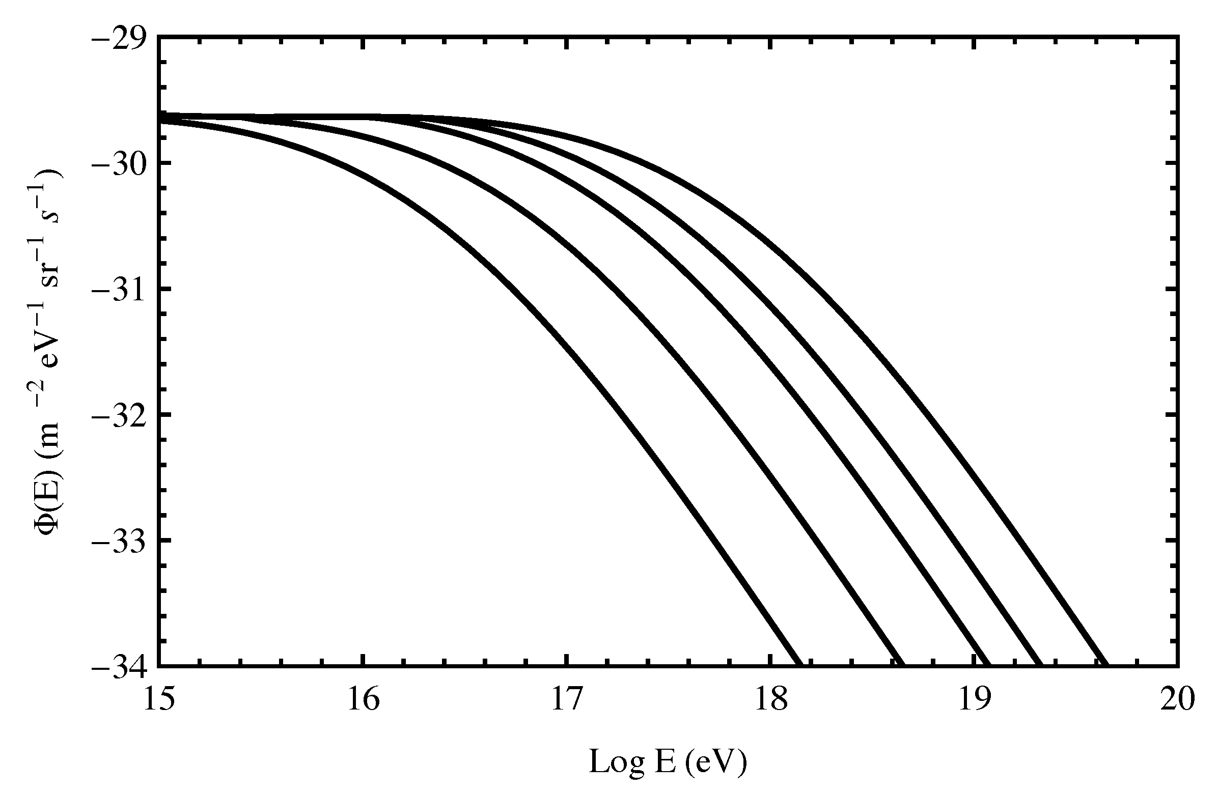
Figure 5.
Diagrams for muon decay (top), charged current-mediated vacuum electron-positron pair emission (VPE) (bottom left) and neutral current-mediated neutrino splitting and VPE (bottom right). Time runs from left to right, and the flavor index i represents , or neutrinos.
Figure 5.
Diagrams for muon decay (top), charged current-mediated vacuum electron-positron pair emission (VPE) (bottom left) and neutral current-mediated neutrino splitting and VPE (bottom right). Time runs from left to right, and the flavor index i represents , or neutrinos.

Figure 6.
Propagated neutrino spectra including energy losses as described in the text [36]. Separately calculated n = 2 neutrino spectra with the VPE case shown in blue and the neutrino splitting case shown in green. The black spectrum takes account of all three processes (redshifting, neutrino splitting and VPE) occurring simultaneously. The rates for all cases are fixed by setting the rest frame threshold energy for VPE at 10 PeV. The neutrino spectra are normalized to the IceCube data both with (gray) and without (black) an estimated flux of prompt atmospheric neutrinos subtracted [49].

© 2017 by the author. Licensee MDPI, Basel, Switzerland. This article is an open access article distributed under the terms and conditions of the Creative Commons Attribution (CC BY) license (http://creativecommons.org/licenses/by/4.0/).
Share and Cite
MDPI and ACS Style
Stecker, F.W. Testing Lorentz Symmetry Using High Energy Astrophysics Observations. Symmetry 2017, 9, 201. https://doi.org/10.3390/sym9100201
AMA Style
Stecker FW. Testing Lorentz Symmetry Using High Energy Astrophysics Observations. Symmetry. 2017; 9(10):201. https://doi.org/10.3390/sym9100201
Chicago/Turabian StyleStecker, Floyd W. 2017. "Testing Lorentz Symmetry Using High Energy Astrophysics Observations" Symmetry 9, no. 10: 201. https://doi.org/10.3390/sym9100201
Note that from the first issue of 2016, this journal uses article numbers instead of page numbers. See further details here.