Scale Effect and Anisotropy Analyzed for Neutrosophic Numbers of Rock Joint Roughness Coefficient Based on Neutrosophic Statistics


1
Key Laboratory of Rock Mechanics and Geohazards, Shaoxing University, 508 Huancheng West Road, Shaoxing 312000, Zhejiang Province, China, [email protected] (J.C.)
2
Department of Electrical and Information Engineering, Shaoxing University, 508 Huancheng West Road, Shaoxing 312000, Zhejiang Province, China
*
Author to whom correspondence should be addressed.
Symmetry 2017, 9(10), 208; https://doi.org/10.3390/sym9100208
Submission received: 21 August 2017
/
Revised: 8 September 2017
/
Accepted: 18 September 2017
/
Published: 1 October 2017
(This article belongs to the Special Issue Neutrosophic Theories Applied in Engineering)
Abstract
:In rock mechanics, the study of shear strength on the structural surface is crucial to evaluating the stability of engineering rock mass. In order to determine the shear strength, a key parameter is the joint roughness coefficient (JRC). To express and analyze JRC values, Ye et al. have proposed JRC neutrosophic numbers (JRC-NNs) and fitting functions of JRC-NNs, which are obtained by the classical statistics and curve fitting in the current method. Although the JRC-NNs and JRC-NN functions contain much more information (partial determinate and partial indeterminate information) than the crisp JRC values and functions in classical methods, the JRC functions and the JRC-NN functions may also lose some useful information in the fitting process and result in the function distortion of JRC values. Sometimes, some complex fitting functions may also result in the difficulty of their expressions and analyses in actual applications. To solve these issues, we can combine the neutrosophic numbers with neutrosophic statistics to realize the neutrosophic statistical analysis of JRC-NNs for easily analyzing the characteristics (scale effect and anisotropy) of JRC values. In this study, by means of the neutrosophic average values and standard deviations of JRC-NNs, rather than fitting functions, we directly analyze the scale effect and anisotropy characteristics of JRC values based on an actual case. The analysis results of the case demonstrate the feasibility and effectiveness of the proposed neutrosophic statistical analysis of JRC-NNs and can overcome the insufficiencies of the classical statistics and fitting functions. The main advantages of this study are that the proposed neutrosophic statistical analysis method not only avoids information loss but also shows its simplicity and effectiveness in the characteristic analysis of JRC.
1. Introduction
The engineering experience shows that rock mass may deform and destroy along the weak structural surfaces. The study of shear strength on the structural surface is crucial to evaluate the stability of engineering rock mass. In order to determine the shear strength in rock mechanics, a key parameter is the joint roughness coefficient (JRC). Since Barton [1] firstly defined the concept of JRC, a lot of methods had been proposed to calculate the JRC value and analyze its anisotropy and scale effect characteristics. Tse et al. [2] gave the linear regression relationship between the JRC value and the root mean square (Z2). Then, Zhang et al. [3] improved the root mean square (Z2) by considering the inclination angle, amplitude of asperities, and their directions, and then introduced a new roughness index (λ) by using the modified root mean square (Z2’) to calculate JRC values. To quantify the anisotropic roughness of joint surfaces effectively, a variogram function and a new index were proposed by Chen et al. [4] based on the digital image processing technique, and then they also studied the scale effect by calculating the JRC values of different sample lengths [5]. However, all of these traditional methods do not consider the uncertainties of JRC values in real rock engineering practice.
Recently, Ye et al. [6] not only utilized the crisp average value to express JRC by using traditional statistical methods, but also considered its interval range (indeterminate range) to express the indeterminate information of JRC by means of the neutrosophic function/interval function. They [6] firstly applied the neutrosophic function to calculate JRC values and shear strength, and got the relations between the sampling length and the maximum JRC values and between the sampling length and the minimum JRC values, and then established the neutrosophic functions (thick/interval functions) of JRC and shear strength. However, these thick/interval functions cannot express such an indeterminate function containing the parameters of neutrosophic numbers (NNs) (i.e., indeterminate parameters), where NN is composed of its determinate part a and its indeterminate part bI with indeterminacy I and as denoted by z = a + bI for a, b R (R is all real numbers) [7,8,9]. Obviously, NN is a very useful mathematical tool for the expression of the partial determinate and/or partial indeterminate information in engineering problems. After that, Ye et al. [10] further proposed two NN functions to express the anisotropic ellipse and logarithmic equations of JRC values corresponding to an actual case and to analyze the anisotropy and scale effect of JRC values by the derivative of the two NN functions, and then they further presented a NN function with two-variables so as to express the indeterminate information of JRC values comprehensively in the sample sizes and measurement orientations, and then they analyzed both the anisotropy and scale effect of JRC values simultaneously by the partial derivative of the NN function with two-variables. However, all of these NN functions are obtained by fitting curves of the measured values, where they may still lose some useful information between 3% and 16% in the fitting process and lack a higher fitting accuracy although the fitting degrees of these functions lie in the interval [84%, 97%] in actual applications [10]. Sometimes, some complex fitting functions may also result in the difficulty of their expressions and analyses in actual applications [10]. To overcome these insufficiencies, it is necessary to improve the expression and analysis methods for the JRC values by some new statistical method so that we can retain more vague, incomplete, imprecise, and indeterminate information in the expression and analysis of JRC and avoid the information loss and distortion phenomenon of JRC values. Thus, the neutrosophic interval statistical number (NISN) presented by Ye et al. [11] is composed of both NN and interval probability, and then it only expresses the JRC value with indeterminate information, but they lack the characteristic analysis of JRC values in [11].
However, determinate and/or indeterminacy information is often presented in the real world. Hence, the NNs introduced by Smarandache [7,8,9] are very suitable for describing determinate and indeterminate information. Then, the neutrosophic statistics presented in [9] is different from classical statistics. The former can deal with indeterminate statistical problems, while the latter cannot do them and can only obtain the crisp values. As mentioned above, since there exist some insufficiencies in the existing analysis methods of JRC, we need a new method to overcome the insufficiencies. For this purpose, we originally propose a neutrosophic statistical method of JRC-NNs to indirectly analyze the scale effect and anisotropy of JRC values by means of the neutrosophic average values and standard deviations of JRC-NNs (JRC values), respectively, to overcome the insufficiencies of existing analysis methods. The main advantages of this study are that the proposed neutrosophic statistical analysis method not only avoid information loss, but also show its simplicity and effectiveness in the characteristic analysis of JRC values.
The rest of this paper is organized as follows. Section 2 introduces some basic concepts of NNs and gives the neutrosophic statistical algorithm to calculate the neutrosophic average value and standard deviation of NNs. Section 3 introduces the source of the JRC data and JRC-NNs in an actual case, where the JRC-NNs of 24 measurement orientations in each sample length and 10 sample lengths in each measurement orientation will be used for neutrosophic statistical analysis of JRC-NNs in the actual case study. In Section 4, the neutrosophic average values and standard deviations of the 24 JRC-NNs of different measurement orientations in each sample length are given based on the proposed neutrosophic statistical algorithm and are used for the scale effect analysis of JRC values. In Section 5, the neutrosophic average values and standard deviations of the 10 JRC-NNs of different sample lengths in each measurement orientations are given based on the proposed neutrosophic statistical algorithm and used for the anisotropic analysis of JRC values. Finally, concluding remarks are given in Section 6.
2. Basic Concepts and Neutrosophic Statistical Algorithm of NNs
NNs and neutrosophic statistics are firstly proposed by Smarandache [7,8,9]. This section will introduce some basic concepts of NNs and give the neutrosophic statistical algorithm of NNs to calculate the neutrosophic average value and the standard deviation of NNs for the neutrosophic statistical analysis of JRC-NNs in the following study.
A NN z = a + bI consists of a determinate part a and an indeterminate part bI, where a and b are real numbers and I [IL, IU] is indeterminacy. It is clear that the NN can express the determinate and/or indeterminate information. Here is a numerical example. A NN is z = 5 + 6I for I [0, 0.3]. Then, the NN is z [5, 6.8] for I [0, 0.3] and its possible range/interval is z = [5, 6.8], where its determinate part is 5 and its indeterminate part is 6I. For the numerical example, z = 5 + 6I for I [0, 0.3] can be also expressed as another form z = 5 + 3I for I [0, 0.6]. Therefore, we can specify some suitable interval range [IL, IU] for the indeterminacy I according to the different applied demands to adapt the actual representation. In fact, NN is a changeable interval number depending on the indeterminacy I [IL, IU].
As we know, data in classical statistics are determinate values/crisp values. On the contrary, data in neutrosophic statistics are interval values/indeterminate values/NNs, which contain indeterminacy. If there is no indeterminacy or crisp value in data, neutrosophic statistics is consistent with classical statistics. Let us consider an example of neutrosophic statistics in the following.
Assume that four NNs are z1 = 1 + 2I, z2 = 2 + 3I, z3 = 3 + 4I, and z4 = 4 + 5I for I [0, 0.2], then the average value of these four neutrosophic numbers can be obtained by the following calculational steps:
Firstly, the average value of the four determinate parts is obtained by the following calculation:
Secondly, the average value of the four coefficients in the indeterminate parts is yielded by the following calculation:
Finally, the neutrosophic average value of the four NNs is given as follows:
This neutrosophic average value is also called the average NN [9], which still includes its determinate and indeterminate information rather than a crisp value.
However, it is difficult to use the Smarandache’s neutrosophic statistics for engineering applications. Thus, Ye et al. [12] presented some new operations of NNs to make them suitable for engineering applications.
Let two NNs be z1 = a1 + b1I and z2 = a2 + b2I for I [IL, IU]. Then, Ye et al. [12] proposed their basic operations:
Then, these basic operations are different from the ones introduced in [9], and this makes them suitable for engineering applications.
Based on Equation (1), we can give the neutrosophic statistical algorithm of the neutrosophic average value and standard deviation of NNs.
Let zi = ai + biI (i = 1, 2,…, n) be a group of NNs for I [IL, IU], then their neutrosophic average value and standard deviation can be calculated by the following neutrosophic statistical algorithm:
Step 1: Calculate the neutrosophic average value of ai (i = 1, 2,…, n):
Step 2: Calculate the average value of bi (i = 1, 2,…, n):
Step 3: Obtain the neutrosophic average value:
Step 4: Get the differences between zi (i = 1, 2,…, n) and :
Step 5: Calculate the square of all the differences between zi (i = 1, 2,…, n) and :
Step 6: Calculate the neutrosophic standard deviation:
In the following sections, we shall apply the proposed neutrosophic statistical algorithm of NNs to the characteristic analysis of JRC data.
3. JRC Values and JRC-NNs in an Actual Case
As an actual case study in this paper, the original roughness profiles were measured by using profilograph and a roughness ruler [13] on a natural rock joint surface in Changshan County of Zhejiang Province, China. In the actual case, based on a classical statistical method we have obtained the average values μij and standard deviations σij (i = 1, 2,…, 24; j = 1, 2,…, 10) of actually measured data in different sample lengths and different measurement orientations, which are shown in Table 1.
Then, we can use NNs zij = aij + bijI (i = 1, 2,…, 24; j = 1, 2,…, 10) to express the JRC values in each orientation θ and in each sample length L. Various NNs of the JRC values are indicated by the real numbers of aij and bij in zij (i = 1, 2,…, 24; j = 1, 2,…, 10). For convenient neutrosophic statistical analysis, the indeterminacy I is specified as the unified form I [0, 1] in all the JRC-NNs. Thus, there is zij = aij + bijI = μij − σij + 2 σijI (i = 1, 2,…, 24; j = 1, 2,…, 10), where aij = μij − σij is the lower bound of the JRC value and zij may choose a robust range/confidence interval [μij − σij, μij + σij] for the symmetry about the average value μij (see the references [10,11] in detail), and then based on μij and σij in Table 1 aij and bij in zij (i = 1, 2,…, 24; j =1, 2,…, 10) are shown in Table 2. For example, when θ = 0° and L = 10 cm for i = 1 and j = 1, we can obtain from Table 2 that the JRC-NN is z11 = 8.3040 + 4.4771I for I [0, 1].
According to the measurement orientation θ and the sample length L in Table 2, the data in the same column consists of a group of the data in each sample length L, and then there are 10 groups in the JRC-NNs. On the other hand, the data in each row are composed of a group of the data in each measurement orientation θ, and then there are 24 groups in the JRC-NNs. In the following, we shall give the neutrosophic statistical analysis of the JRC-NNs based on the proposed neutrosophic statistical algorithm to reflect their scale effect and anisotropy in the actual case.
4. Scale Effect Analysis in Different Sample Lengths Based on the Neutrosophic Statistical Algorithm
In this section, we give the neutrosophic statistical analysis of JRC-NNs of each column in Table 2 based on the neutrosophic statistical algorithm to reflect the scale effect of JRC-NNs in different sample lengths.
In the neutrosophic statistical analysis of JRC-NNs, we need to calculate the neutrosophic average value and the standard deviation of each group of JRC-NNs in each column by using Equations (2)–(7). To show their calculational procedures in detail, we give the following example.
For example, the neutrosophic average value and standard deviation of the JRC-NNs in L = 10 cm is calculated. Then, we give the following calculational steps based on the neutrosophic statistical algorithm.
Step 1: By Equation (2), calculate the average value of the determinate parts ai1 (i = 1, 2,…, 24) in the JRC-NNs corresponding to the first column as follows:
Step 2: By Equation (3), calculate the average value of the indeterminate coefficients bi1 (i = 1, 2,…, 24) in the JRC-NNs:
Step 3: By Equation (4), obtain the neutrosophic average value of the JRC-NNs in the first column:
Step 4: By Equation (5), calculate the differences between zi1 (i = 1, 2,…, 24) and :
Step 5: By Equation (6), calculate the square of all the differences:
Step 6: By Equation (7), calculate the neutrosophic standard deviation:
Thus, the neutrosophic average value and the standard deviation of the JRC-NNs in the first column are obtained by the above calculational steps. By the similar calculational steps, the neutrosophic average values and standard deviations of JRC-NNs in other columns can be also obtained and all of the results are shown in Table 3. Then, the neutrosophic average values and standard deviations of JRC-NNs in different sample lengths are depicted in Figure 1 and Figure 2.
Figure 1 shows that the neutrosophic average values (ranges) of JRC-NNs decrease with the sample length increases. It is obvious that they can reflect the scale effect in different lengths. In other words, the larger the length L is, the smaller the average value (range) of JRC-NNs is. Thus, the scale effect in different lengths is consistent with that of the literature [10].
In Figure 2, we can see that the neutrosophic standard deviations of JRC-NNs decrease with the sample length increases. Since the standard deviation is used to indicate the dispersion degree of data, the neutrosophic standard deviation in some length L means the dispersion degree of the JRC-NNs. The larger the standard deviation is, the more discrete the JRC-NNs is. Under some sample lengths, its standard deviation means the dispersion degree of the JRC-NNs in different orientations. The larger the neutrosophic standard deviation is, the more obvious the anisotropy of the JRC-NNs under this length is. Hence, the neutrosophic standard deviations of JRC-NNs can also indicate the scale effect of the anisotropy of JRC-NNs. What’s more, when the sample length is large enough, the anisotropy of the JRC values may decrease to some stable tendency. This situation is consistent with the tendency in [10].
Obviously, both neutrosophic average values and neutrosophic standard deviations of JRC-NNs can reflect the scale effect of JRC-NNs. Then, the neutrosophic average values reflect the scale effect of JRC values, while the neutrosophic standard deviations reflect the scale effect of the anisotropy of JRC values.
5. Anisotropic Analysis in Different Measurement Orientations Based on the Neutrosophic Statistical Algorithm
In this section, we give the neutrosophic statistical analysis of JRC-NNs of each row in Table 2 based on the neutrosophic statistical algorithm to reflect the anisotropy of JRC-NNs in different measurement orientations.
To indicate the neutrosophic statistical process, we take the orientation of θ = 0° for i = 1 as an example to show the detailed calculational steps of the neutrosophic average value and the standard deviation of the JRC-NNs in the orientation based on the neutrosophic statistical algorithm.
Step 1: By Equation (2), calculate the average value of the determinate parts a1j (j = 1, 2,…, 10) of the JRC-NNs in the first row (i = 1) as follows:
Step 2: By Equation (3), calculate the average value of b1j (j = 1, 2,…, 10) in the indeterminate parts of the JRC-NNs:
Step 3: By Equation (4), get the neutrosophic average value of the JRC-NNs in the first row:
Step 4: By Equation (5), calculate the differences between z1j (j = 1, 2,…, 10) and :
Step 5: By Equation (6), calculate the square of these differences:
Step 6: By Equation (7), calculate the neutrosophic standard deviation:
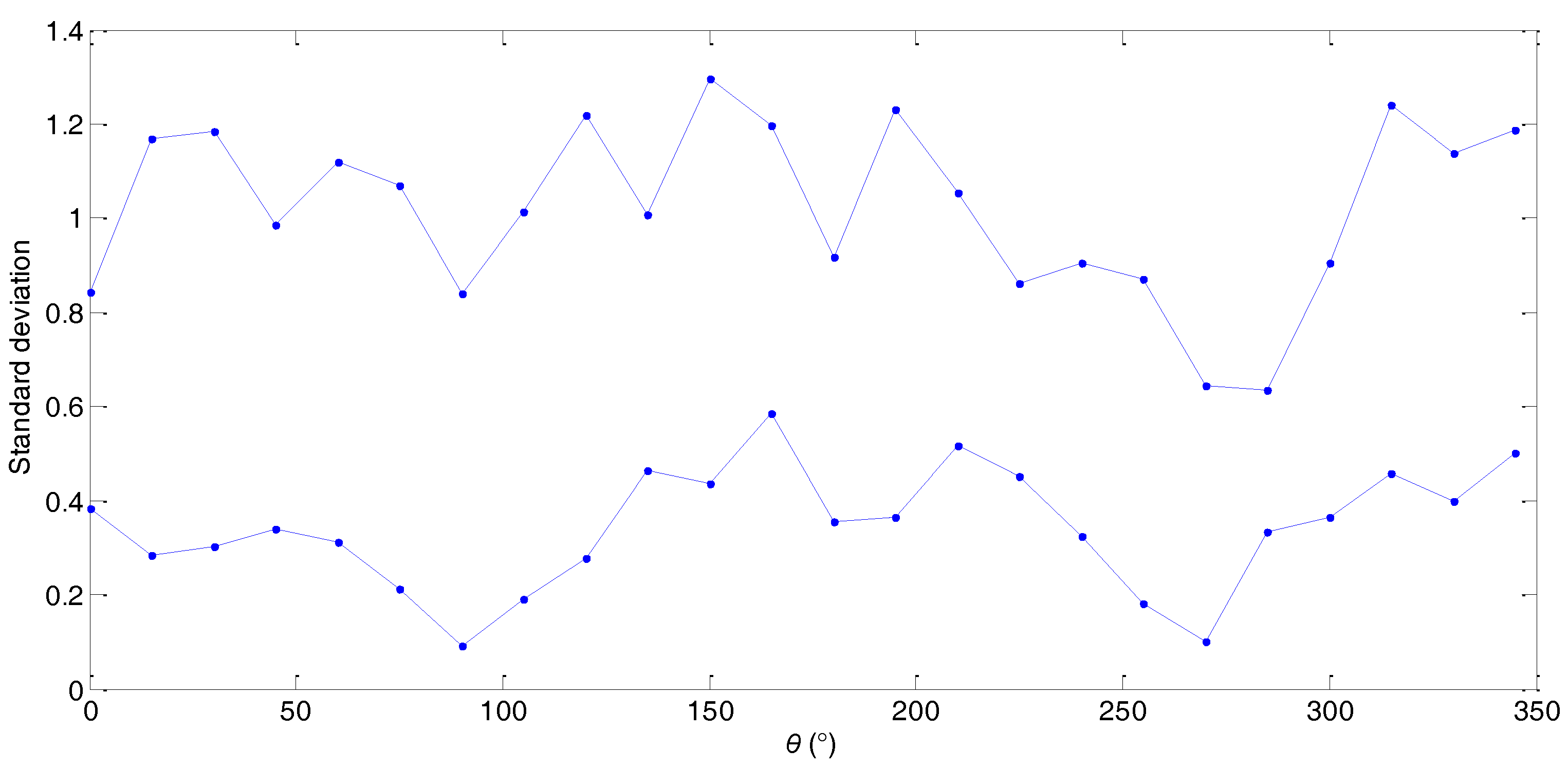
By the similar calculational steps, the neutrosophic average values and standard deviations of JRC-NNs in other rows can be also obtained and all the results are shown in Table 4. Then, the neutrosophic average values and standard deviations of JRC-NNs in different orientations are depicted in Figure 3 and Figure 4.
Figure 3 shows that the neutrosophic average values (ranges) of JRC-NNs are very different in every orientation. Their changing curves look somewhat like trigonometric functions, which show the anisotropy of JRC-NNs.
In Figure 4, the neutrosophic standard deviations indicate the dispersion degrees of JRC-NNs under different sample lengths in some orientation. The larger the neutrosophic standard deviation is, the more discrete the JRC-NNs is. This case indicates that the scale effect of JRC-NNs is more obvious in the orientation. Although the changing curves in Figure 4 are irregular, it is clear that the dispersion degree of each orientation is very different. For example, the neutrosophic standard deviation of θ = 270° is obviously smaller than that of other orientations. Especially, if the JRC-NNs of all rows have the same neutrosophic standard deviations in such a special case, then the two curve area in Figure 4 will be reduced to the area between two parallel lines without the anisotropy in each sample scale.
From the above analysis, it is obvious that the neutrosophic average values and standard deviations of JRC-NNs (JRC values) also imply the anisotropy in different orientations. Thus, the neutrosophic average values reflect the anisotropy of JRC values, while the neutrosophic standard deviations reflect the anisotropy of the scale effect. Obviously, this neutrosophic statistical analysis method is more detailed and more effective than existing methods and avoids the difficulty of the curve fitting and analysis in some complex cases.
6. Conclusion Remarks
According to the JRC data obtained in an actual case and the expressions and operations of JRC-NNs, we provided a new neutrosophic statistical analysis method based on the neutrosophic statistical algorithm of the neutrosophic average values and the standard deviations of JRC-NNs in different columns (different sample lengths) and different rows (different measurement orientations). It is obvious that the two characteristic analyses (scale effect and anisotropy) of JRC values were indicated in this study. For the first characteristic, we analyzed the scale effect of JRC-NNs in different sample lengths, where the neutrosophic average values reflect the scale effect of JRC-NNs, while the neutrosophic standard deviations reflect the scale effect of the anisotropy of JRC-NNs. For the second characteristic, we analyzed the anisotropy of JRC values in different measurement orientations, where the neutrosophic average values reflect the anisotropy of JRC-NNs, while the neutrosophic standard deviations reflect the anisotropy of the scale effect. Therefore, the neutrosophic statistical analysis of the actual case demonstrates that the neutrosophic average values and neutrosophic standard deviations of JRC-NNs can reflect the scale effect and anisotropic characteristics of JRC values reasonably and effectively.
However, the obtained analysis results and the performance benefits of the presented neutrosophic statistical algorithm in this study are summarized as follows:
- (1)
- The neutrosophic statistical analysis method without fitting functions is more feasible and more reasonable than the existing method [10].
- (2)
- The neutrosophic statistical analysis method based on the neutrosophic average values and neutrosophic standard deviations of JRC-NNs can retain much more information and reflect the scale effect and anisotropic characteristics of JRC values in detail.
- (3)
- The presented neutrosophic statistical algorithm can analyze the scale effect and the anisotropy of JRC-NNs (JRC values) directly and effectively so as to reduce the information distortion.
- (4)
- The presented neutrosophic statistical algorithm based on the neutrosophic statistical averages and standard deviations of JRC-NNs is more convenient and simpler than the existing curve fitting and derivative analysis of JRC-NN functions in [10].
- (5)
- The presented neutrosophic statistical algorithm can overcome the insufficiencies of the existing method in the fitting and analysis process [10].
- (6)
From what has been discussed above, the proposed neutrosophic statistical analysis method of JRC-NNs provides a more convenient and feasible new way for the scale effect and anisotropic characteristic analysis of JRC values in rock mechanics.
Acknowledgments
This paper was supported by the National Natural Science Foundation of China (Nos. 71471172, 41427802).
Author Contributions
Jun Ye proposed the neutrosophic statistical algorithm; Jun Ye and Jiqian Chen gave the neutrosophic statistical analysis of the actual case to indicate the scale effect and anisotropic characteristics of JRC values in rock mechanics; Shigui Du and Jiqian Chen provided actual measuring data and statistical analysis in the actual case; we wrote the paper together.
Conflicts of Interest
The authors declare no conflicts of interest.
References
- Barton, N. Review of a new shear-strength criterion for rock joints. Eng. Geol. 1973, 7, 287–332. [Google Scholar] [CrossRef]
- Tse, R.; Cruden, D.M. Estimating joint roughness coefficients. Int. J. Rock Mech. Min. Sci. Geomech. Abstr. 1979, 16, 303–307. [Google Scholar] [CrossRef]
- Zhang, G.C.; Karakus, M.; Tang, H.M.; Ge, Y.F.; Zhang, L. A new method estimating the 2D joint roughness coefficient for discontinuity surfaces in rock masses. Int. J. Rock Mech. Min. Sci. 2014, 72, 191–198. [Google Scholar] [CrossRef]
- Chen, S.J.; Zhu, W.C.; Yu, Q.L.; Liu, X.G. Characterization of anisotropy of joint surface roughness and aperture by variogram approach based on digital image processing technique. Rock Mech. Rock Eng. 2016, 49, 855–876. [Google Scholar] [CrossRef]
- Chen, S.J.; Zhu, W.C.; Liu, S.X.; Zhang, F.; Guo, L.F. Anisotropy and size effects of surface roughness of rock joints. Chin. J. Rock Mech. Eng. 2015, 34, 57–66. [Google Scholar]
- Ye, J.; Yong, R.; Liang, Q.F.; Huang, M.; Du, S.G. Neutrosophic functions of the joint roughness coefficient and the shear strength: A case study from the pyroclastic rock mass in Shaoxing City, China. Math. Probl. Eng. 2016. [Google Scholar] [CrossRef]
- Smarandache, F. Neutrosophy: Neutrosophic Probability, Set, and Logic; American Research Press: Rehoboth, DE, USA, 1998. [Google Scholar]
- Smarandache, F. Introduction to Neutrosophic Measure, Neutrosophic Integral, and Neutrosophic Probability; Sitech & Education Publisher: Craiova, Romania, 2013. [Google Scholar]
- Smarandache, F. Introduction to Neutrosophic Statistics; Sitech & Education Publisher: Craiova, Romania, 2014. [Google Scholar]
- Ye, J.; Chen, J.Q.; Yong, R.; Du, S.G. Expression and analysis of joint roughness coefficient using neutrosophic number functions. Information 2017, 8, 69. [Google Scholar] [CrossRef]
- Chen, J.Q.; Ye, J.; Du, S.G.; Yong, R. Expressions of rock joint roughness coefficient using neutrosophic interval statistical numbers. Symmetry 2017, 9, 123. [Google Scholar] [CrossRef]
- Ye, J. Neutrosophic number linear programming method and its application under neutrosophic number environments. Soft Comput. 2017. [Google Scholar] [CrossRef]
- Du, S.G.; Hu, Y.J.; Hu, X.F. Measurement of joint roughness coefficient by using profilograph and roughness ruler. J. Earth Sci. 2009, 20, 890–896. [Google Scholar] [CrossRef]
Figure 1.
The neutrosophic average values of JRC-NNs in different sample lengths L.
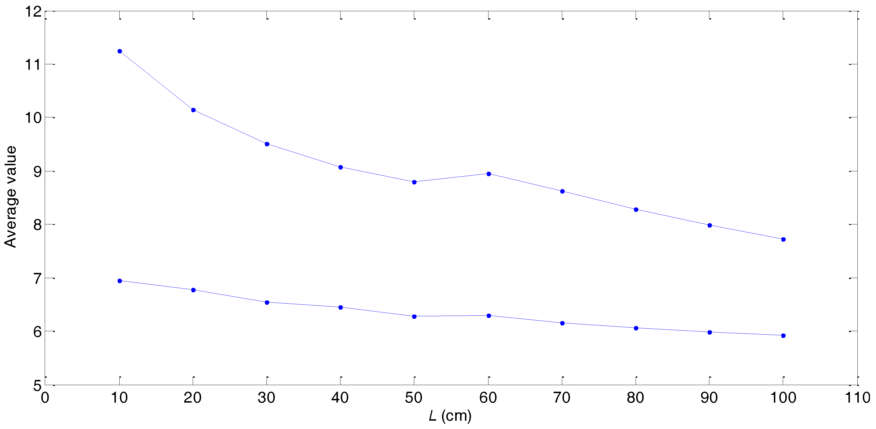
Figure 2.
The neutrosophic standard deviations of JRC-NNs in different sample lengths L.
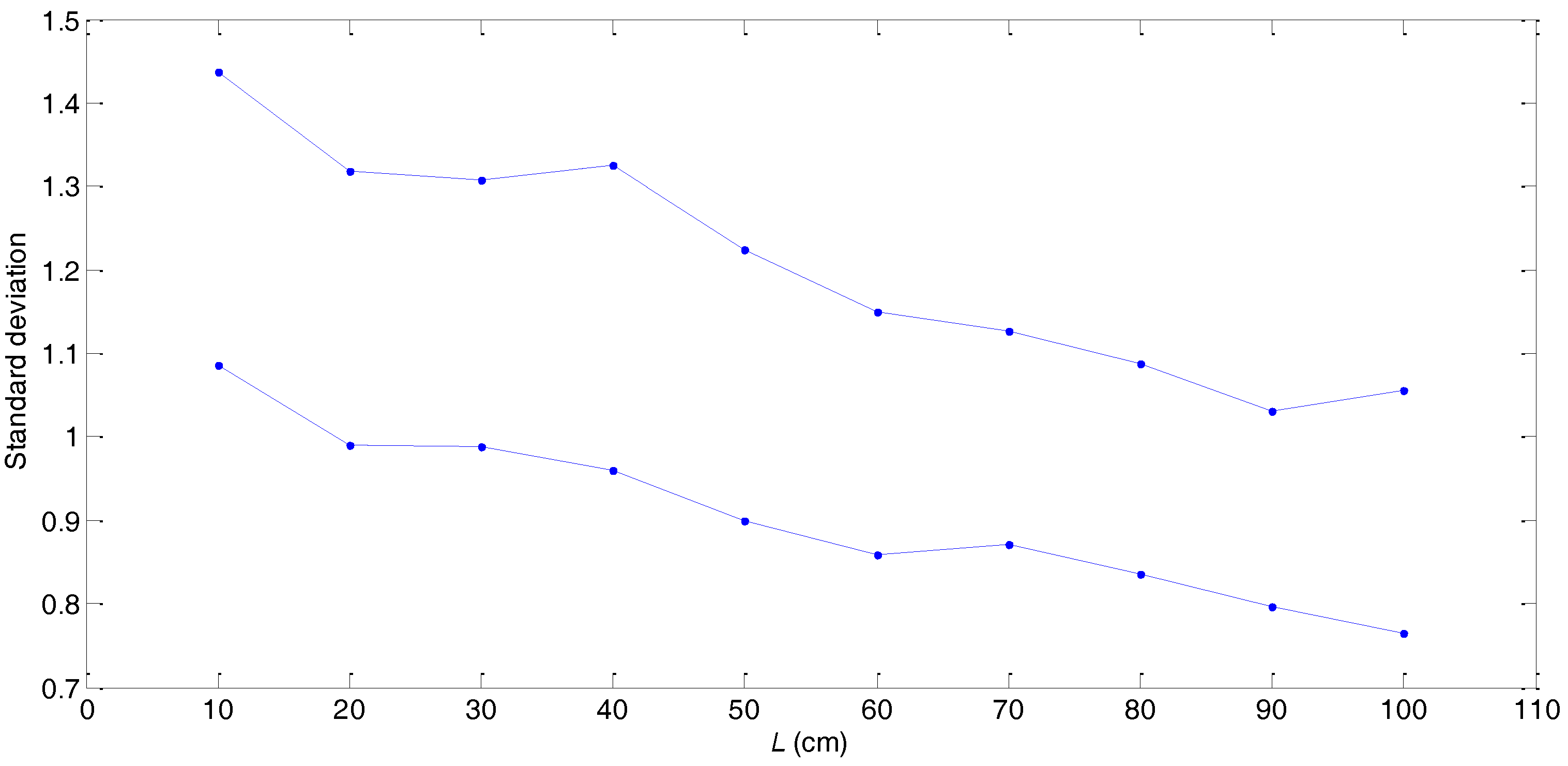
Figure 3.
The neutrosophic average values of JRC-NNs in different orientations θ.
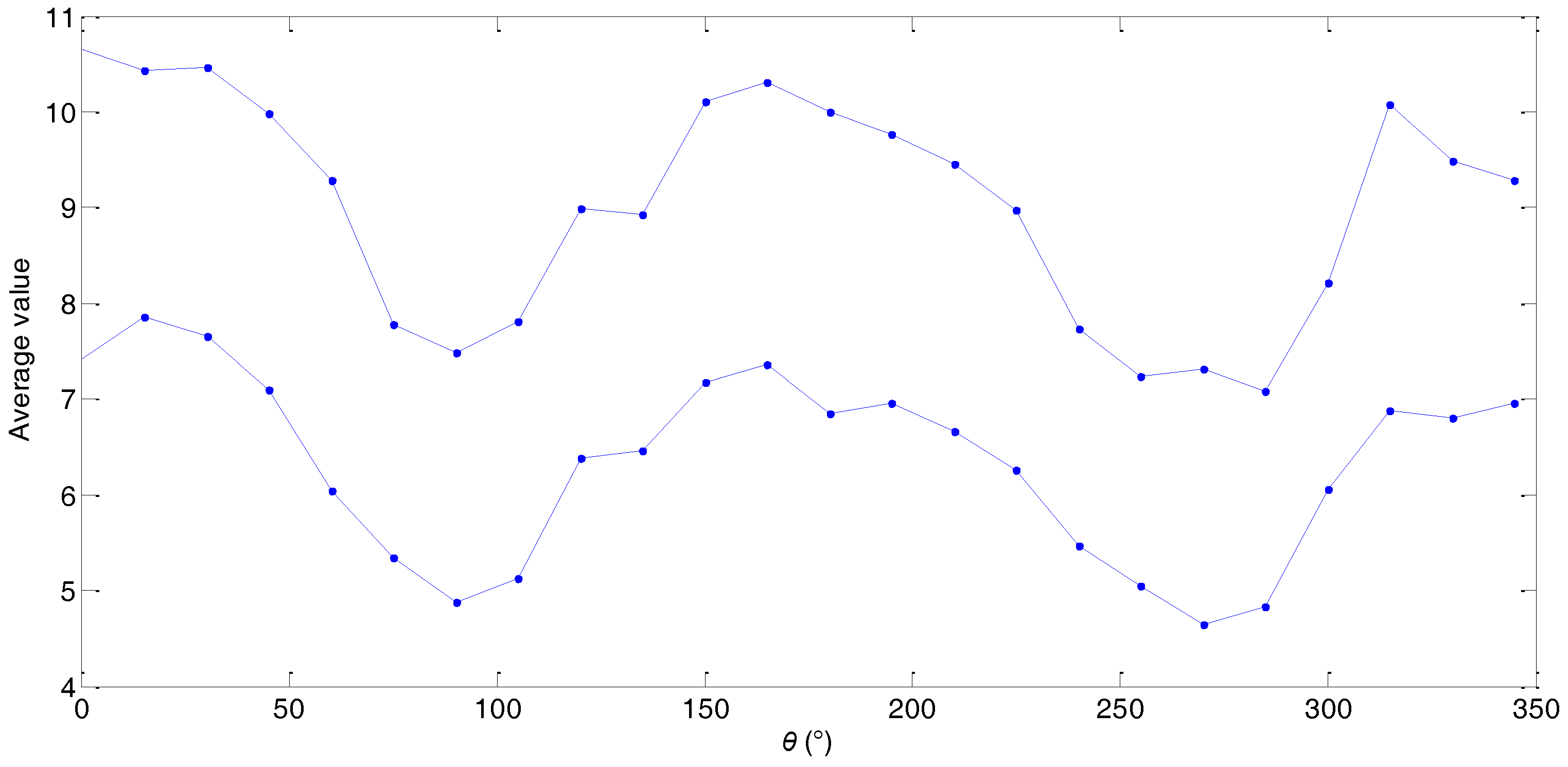
Figure 4.
The neutrosophic standard deviations of JRC-NNs in different orientations θ.

Table 1.
The average values μij and standard deviations σij of actually measured data in different sample lengths L and different measurement orientations θ.
Table 1.
The average values μij and standard deviations σij of actually measured data in different sample lengths L and different measurement orientations θ.
| L | 10 cm | 20 cm | 30 cm | 40 cm | 50 cm | 60 cm | 70 cm | 80 cm | 90 cm | 100 cm | ||||||||||
|---|---|---|---|---|---|---|---|---|---|---|---|---|---|---|---|---|---|---|---|---|
| θ | μi1 | σi1 | μi2 | σi2 | μi3 | σi3 | μi4 | σi4 | μi5 | σi5 | μi6 | σi6 | μi7 | σi7 | μi8 | σi8 | μi9 | σi9 | μi10 | σi10 |
| 0° | 10.5425 | 2.2385 | 9.6532 | 1.7162 | 9.2733 | 1.5227 | 8.9745 | 1.7092 | 8.8222 | 1.6230 | 8.8016 | 1.6069 | 8.6815 | 1.6066 | 8.6009 | 1.5043 | 8.5681 | 1.3465 | 8.4630 | 1.2806 |
| 15° | 10.7111 | 2.2392 | 9.9679 | 1.7379 | 9.3433 | 1.5555 | 9.2708 | 1.2743 | 9.2299 | 1.2850 | 8.9729 | 1.3071 | 8.8332 | 1.1706 | 8.5868 | 0.9413 | 8.3604 | 0.7673 | 8.1404 | 0.6372 |
| 30° | 10.5943 | 2.3528 | 9.9289 | 2.0286 | 9.5715 | 1.6665 | 9.1209 | 1.4207 | 9.0920 | 1.4119 | 8.6006 | 0.9899 | 8.7596 | 1.1489 | 8.5713 | 1.0776 | 8.2927 | 1.0128 | 8.1041 | 0.9664 |
| 45° | 9.9244 | 2.3120 | 9.2005 | 1.7237 | 9.0081 | 1.6464 | 8.5078 | 1.1376 | 8.3336 | 1.431 | 8.6237 | 1.3427 | 8.3262 | 1.2184 | 8.0768 | 1.2717 | 7.8458 | 1.2096 | 7.5734 | 1.1294 |
| 60° | 9.0253 | 2.4592 | 8.4047 | 1.9813 | 7.8836 | 1.8199 | 7.7941 | 1.8829 | 7.1873 | 1.167 | 8.2678 | 1.7830 | 7.3595 | 1.5956 | 7.1381 | 1.4082 | 6.8722 | 1.2178 | 6.7131 | 0.9627 |
| 75° | 7.9352 | 2.1063 | 7.4604 | 1.7756 | 6.7725 | 1.4153 | 6.3056 | 1.0241 | 6.5446 | 1.2140 | 6.4993 | 1.3108 | 6.2440 | 1.1208 | 6.0933 | 0.9171 | 5.9499 | 0.7311 | 5.8317 | 0.5855 |
| 90° | 7.0467 | 2.4054 | 6.6915 | 1.8482 | 6.3378 | 1.4743 | 5.9993 | 1.1700 | 6.1481 | 1.1920 | 6.0893 | 1.1850 | 5.9543 | 1.1021 | 5.8932 | 0.9630 | 5.8259 | 0.9181 | 5.8219 | 0.8355 |
| 105° | 7.7766 | 2.4105 | 7.2221 | 1.7560 | 6.6770 | 1.2608 | 6.2318 | 0.985 | 6.4634 | 1.2288 | 6.4609 | 1.5029 | 6.1670 | 1.3236 | 5.9923 | 1.1016 | 5.8903 | 0.9868 | 5.8359 | 0.8479 |
| 120° | 9.1324 | 2.3250 | 8.5206 | 1.8963 | 8.1998 | 1.5792 | 7.9671 | 1.4094 | 7.3207 | 1.0418 | 7.8245 | 1.1807 | 7.2472 | 1.0637 | 7.0649 | 0.9507 | 6.8537 | 0.8122 | 6.6909 | 0.7715 |
| 135° | 9.2258 | 1.9104 | 8.5670 | 1.5412 | 8.0898 | 1.3452 | 7.8194 | 0.9910 | 7.3735 | 0.9848 | 7.6660 | 1.2845 | 7.3846 | 1.1608 | 7.0872 | 1.1589 | 6.9154 | 1.0345 | 6.7586 | 0.9157 |
| 150° | 10.4673 | 2.4365 | 9.5650 | 1.9065 | 8.9102 | 1.6863 | 8.9059 | 1.4562 | 8.3930 | 1.1855 | 8.8162 | 1.5870 | 8.2064 | 1.3432 | 8.0153 | 1.1287 | 7.6556 | 1.0101 | 7.4443 | 0.9080 |
| 165° | 10.6035 | 2.2090 | 9.9647 | 1.6606 | 9.5320 | 1.5695 | 8.8760 | 1.5994 | 8.6121 | 1.4899 | 8.6463 | 1.5942 | 8.3931 | 1.3637 | 8.1107 | 1.2203 | 7.9051 | 1.0893 | 7.7175 | 1.0050 |
| 180° | 9.8501 | 2.1439 | 9.0984 | 1.8556 | 8.7574 | 1.7300 | 8.6002 | 1.6753 | 8.2973 | 1.5862 | 8.1266 | 1.6278 | 7.9647 | 1.4864 | 7.8981 | 1.3395 | 7.8338 | 1.1935 | 7.8291 | 1.0616 |
| 195° | 9.9383 | 2.2254 | 9.2299 | 1.8331 | 8.6781 | 1.6791 | 8.7993 | 1.4556 | 8.5308 | 1.5551 | 8.1016 | 1.5598 | 7.9219 | 1.2559 | 7.6562 | 0.9674 | 7.4610 | 0.8060 | 7.3131 | 0.7402 |
| 210° | 9.5903 | 1.9444 | 8.9414 | 1.5298 | 8.6532 | 1.6227 | 8.2601 | 1.5626 | 8.2065 | 1.5438 | 7.3828 | 1.2507 | 7.7527 | 1.2989 | 7.5050 | 1.1484 | 7.2495 | 1.0876 | 7.0479 | 0.9558 |
| 225° | 8.9167 | 1.9764 | 8.2550 | 1.4256 | 8.1330 | 1.4751 | 7.7012 | 1.2124 | 7.6798 | 1.4502 | 7.4365 | 1.1748 | 7.3183 | 1.2086 | 7.1309 | 1.2749 | 6.8652 | 1.2190 | 6.6742 | 1.1571 |
| 240° | 7.8582 | 1.8456 | 7.3032 | 1.4385 | 6.8241 | 1.1626 | 6.7427 | 1.2022 | 6.3250 | 0.8971 | 6.8181 | 1.1123 | 6.3526 | 1.0430 | 6.1521 | 0.9953 | 5.9138 | 0.8906 | 5.7515 | 0.7329 |
| 255° | 7.2166 | 1.9341 | 6.8638 | 1.3901 | 6.3349 | 1.2705 | 6.1050 | 1.0350 | 6.0333 | 0.9671 | 6.0693 | 1.1394 | 5.8924 | 0.9417 | 5.7122 | 0.8153 | 5.7803 | 0.8598 | 5.3946 | 0.5627 |
| 270° | 6.8025 | 2.1165 | 6.3123 | 1.6374 | 6.0061 | 1.3786 | 5.8815 | 1.3700 | 5.7871 | 1.1783 | 5.9707 | 1.2858 | 5.8530 | 1.2711 | 5.7376 | 1.1886 | 5.8259 | 0.9181 | 5.5856 | 1.0273 |
| 285° | 7.0061 | 1.5474 | 6.4941 | 1.1183 | 6.1107 | 0.9586 | 5.8455 | 0.9821 | 5.7563 | 0.9033 | 6.0606 | 1.3603 | 5.8403 | 1.2714 | 5.6386 | 1.1359 | 5.4716 | 1.0374 | 5.3629 | 0.9501 |
| 300° | 8.4720 | 1.7448 | 7.8124 | 1.3531 | 7.5303 | 1.2127 | 7.2813 | 1.0247 | 6.9533 | 1.1089 | 7.0673 | 0.8880 | 6.8002 | 0.9202 | 6.6414 | 0.8727 | 6.4460 | 0.8434 | 6.3104 | 0.7904 |
| 315° | 10.1428 | 2.4790 | 9.4554 | 2.1149 | 8.9644 | 1.7308 | 8.5698 | 1.4949 | 8.1224 | 1.4089 | 8.6863 | 1.5162 | 8.3659 | 1.5934 | 7.6582 | 1.3811 | 7.4641 | 1.1563 | 7.3537 | 1.0960 |
| 330° | 9.8295 | 2.2844 | 9.0011 | 1.6139 | 8.3261 | 1.6005 | 8.3290 | 1.3232 | 7.8712 | 1.2376 | 8.0526 | 1.2755 | 7.9134 | 1.1209 | 7.6498 | 1.0157 | 7.3466 | 0.9740 | 7.0927 | 0.9342 |
| 345° | 9.6831 | 2.0192 | 9.1761 | 1.6305 | 8.7732 | 1.1686 | 8.4741 | 1.1887 | 7.8597 | 1.1436 | 7.8485 | 1.0332 | 7.7270 | 1.0174 | 7.4667 | 0.9254 | 7.1781 | 0.821 | 7.0038 | 0.7346 |
Table 2.
The values of aij and bij in JRC neutrosophic numbers (JRC-NNs) zij (i = 1, 2,…, 24; j =1, 2,…, 10) for each orientation θ and each sample length L.
Table 2.
The values of aij and bij in JRC neutrosophic numbers (JRC-NNs) zij (i = 1, 2,…, 24; j =1, 2,…, 10) for each orientation θ and each sample length L.
| L | 10 cm | 20 cm | 30 cm | 40 cm | 50 cm | 60 cm | 70 cm | 80 cm | 90 cm | 100 cm | ||||||||||
|---|---|---|---|---|---|---|---|---|---|---|---|---|---|---|---|---|---|---|---|---|
| θ | ai1 | bi1 | ai2 | bi2 | ai3 | bi3 | ai4 | bi4 | ai5 | bi5 | ai6 | bi6 | ai7 | bi7 | ai8 | bi8 | ai9 | bi9 | ai10 | bi10 |
| 0° | 8.3040 | 4.4771 | 7.9370 | 3.4325 | 7.7506 | 3.0454 | 7.2653 | 3.4184 | 7.1992 | 3.2459 | 7.1947 | 3.2138 | 7.0750 | 3.2132 | 7.0966 | 3.0085 | 7.2216 | 2.6930 | 7.1824 | 2.5612 |
| 15° | 8.4719 | 4.4784 | 8.2300 | 3.4759 | 7.7878 | 3.1110 | 7.9964 | 2.5487 | 7.9449 | 2.5700 | 7.6657 | 2.6142 | 7.6627 | 2.3412 | 7.6456 | 1.8825 | 7.5931 | 1.5347 | 7.5032 | 1.2745 |
| 30° | 8.2415 | 4.7057 | 7.9003 | 4.0572 | 7.9051 | 3.3330 | 7.7002 | 2.8414 | 7.6801 | 2.8239 | 7.6107 | 1.9798 | 7.6107 | 2.2977 | 7.4938 | 2.1552 | 7.2799 | 2.0256 | 7.1377 | 1.9328 |
| 45° | 7.6124 | 4.6240 | 7.4768 | 3.4474 | 7.3616 | 3.2929 | 7.3701 | 2.2753 | 6.9018 | 2.8636 | 7.2810 | 2.6853 | 7.1078 | 2.4369 | 6.8051 | 2.5434 | 6.6362 | 2.4192 | 6.4440 | 2.2589 |
| 60° | 6.5660 | 4.9185 | 6.4234 | 3.9627 | 6.0638 | 3.6397 | 5.9112 | 3.7658 | 6.0203 | 2.3341 | 6.4848 | 3.5660 | 5.7639 | 3.1912 | 5.7299 | 2.8163 | 5.6544 | 2.4355 | 5.7504 | 1.9253 |
| 75° | 5.8289 | 4.2126 | 5.6847 | 3.5513 | 5.3573 | 2.8306 | 5.2815 | 2.0483 | 5.3307 | 2.4279 | 5.1885 | 2.6216 | 5.1232 | 2.2416 | 5.1762 | 1.8342 | 5.2188 | 1.4622 | 5.2462 | 1.1710 |
| 90° | 4.6413 | 4.8108 | 4.8432 | 3.6965 | 4.8635 | 2.9486 | 4.8293 | 2.3399 | 4.9561 | 2.3841 | 4.9043 | 2.3701 | 4.8522 | 2.2043 | 4.9302 | 1.9260 | 4.9078 | 1.8362 | 4.9865 | 1.6709 |
| 105° | 5.3661 | 4.821 | 5.4661 | 3.5119 | 5.4162 | 2.5216 | 5.2460 | 1.9717 | 5.2346 | 2.4576 | 4.9580 | 3.0058 | 3.0054 | 2.6472 | 4.8907 | 2.2031 | 4.9034 | 1.9737 | 4.9881 | 1.6957 |
| 120° | 6.8074 | 4.6500 | 6.6243 | 3.7926 | 6.6206 | 3.1584 | 6.5577 | 2.8188 | 6.2789 | 2.0837 | 6.6438 | 2.3614 | 6.1834 | 2.1274 | 6.1142 | 1.9014 | 6.0415 | 1.6243 | 5.9194 | 1.5430 |
| 135° | 7.3153 | 3.8208 | 7.0258 | 3.0824 | 6.7446 | 2.6904 | 6.8283 | 1.9821 | 6.3887 | 1.9696 | 6.3815 | 2.5690 | 6.2238 | 2.3216 | 5.9283 | 2.3178 | 5.8810 | 2.0689 | 5.8429 | 1.8314 |
| 150° | 8.0308 | 4.8731 | 7.6585 | 3.8130 | 7.2240 | 3.3725 | 7.4497 | 2.9125 | 7.2075 | 2.3710 | 7.2292 | 7.2291 | 6.8633 | 2.6863 | 6.8866 | 2.2573 | 6.6454 | 2.0203 | 6.5363 | 1.8161 |
| 165° | 8.3945 | 4.4180 | 8.3040 | 3.3213 | 7.9625 | 3.1391 | 7.2766 | 3.1988 | 7.1222 | 2.9799 | 7.0521 | 3.1884 | 7.0294 | 2.7274 | 6.8904 | 2.4406 | 6.8158 | 2.1787 | 6.7124 | 2.0101 |
| 180° | 7.7062 | 4.2877 | 7.2427 | 3.7113 | 7.0273 | 3.4601 | 6.9249 | 3.3506 | 6.7111 | 3.1724 | 6.4988 | 3.2556 | 6.4782 | 2.9729 | 6.5586 | 2.6790 | 6.6403 | 2.3871 | 6.7675 | 2.1232 |
| 195° | 7.7130 | 4.4507 | 7.3968 | 3.6661 | 6.9990 | 3.3583 | 7.3437 | 2.9113 | 6.9757 | 3.1102 | 6.5419 | 3.1195 | 6.6660 | 2.5119 | 6.6888 | 1.9348 | 6.6550 | 1.6120 | 6.5729 | 1.4803 |
| 210° | 7.6459 | 3.8887 | 7.4116 | 3.0596 | 7.0305 | 3.2453 | 6.6975 | 3.1252 | 6.6628 | 3.0875 | 6.1321 | 2.5014 | 6.4538 | 2.5977 | 6.3566 | 2.2967 | 6.1619 | 2.1752 | 6.0921 | 1.9116 |
| 225° | 6.9402 | 3.9529 | 6.8294 | 2.8512 | 6.6580 | 2.9502 | 6.4888 | 2.4248 | 6.2296 | 2.9004 | 6.2617 | 2.3495 | 6.1097 | 2.4172 | 5.8560 | 2.5498 | 5.6462 | 2.4379 | 5.5170 | 2.3143 |
| 240° | 6.0125 | 3.6913 | 5.8648 | 2.8769 | 5.6615 | 2.3252 | 5.5405 | 2.4044 | 5.4280 | 1.7941 | 5.7058 | 2.2246 | 5.3096 | 2.0861 | 5.1568 | 1.9906 | 5.0231 | 1.7812 | 5.0186 | 1.4658 |
| 255° | 5.2825 | 3.8683 | 5.4738 | 2.7801 | 5.0644 | 2.5410 | 5.0700 | 2.0701 | 5.0662 | 1.9343 | 4.9300 | 2.2788 | 4.9507 | 1.8834 | 4.8968 | 1.6307 | 4.9204 | 1.7197 | 4.8319 | 1.1253 |
| 270° | 4.6859 | 4.2330 | 4.6748 | 3.2749 | 4.6275 | 2.7571 | 4.5115 | 2.7401 | 4.6088 | 2.3565 | 4.6849 | 2.5716 | 4.5820 | 2.5422 | 4.5490 | 2.3772 | 4.9078 | 1.8362 | 4.5584 | 2.0545 |
| 285° | 5.4587 | 3.0948 | 5.3757 | 2.2367 | 5.1521 | 1.9172 | 4.8634 | 1.9642 | 4.8530 | 1.8066 | 4.7003 | 2.7205 | 4.5688 | 2.5429 | 4.5027 | 2.2719 | 4.4341 | 2.0749 | 4.4128 | 1.9002 |
| 300° | 6.7272 | 3.4897 | 6.4594 | 2.7061 | 6.3176 | 2.4254 | 6.2566 | 2.0494 | 5.8444 | 2.2178 | 6.1793 | 1.7760 | 5.8800 | 1.8404 | 5.7687 | 1.7453 | 5.6025 | 1.6869 | 5.5200 | 1.5808 |
| 315° | 7.6638 | 4.9579 | 7.3405 | 4.2297 | 7.2336 | 3.4616 | 7.0749 | 2.9898 | 6.7135 | 2.8178 | 7.1701 | 3.0324 | 6.7725 | 3.1868 | 6.2771 | 2.7622 | 6.3079 | 2.3125 | 6.2577 | 2.1921 |
| 330° | 7.5450 | 4.5689 | 7.3872 | 3.2277 | 6.7256 | 3.2009 | 7.0058 | 2.6464 | 6.6335 | 2.4751 | 6.7770 | 2.5510 | 6.7925 | 2.2418 | 6.6340 | 2.0314 | 6.3726 | 1.9480 | 6.1586 | 1.8684 |
| 345° | 7.6639 | 4.0383 | 7.5456 | 3.2610 | 7.6046 | 2.3372 | 7.2854 | 2.3774 | 6.7161 | 2.2872 | 6.8153 | 2.0664 | 6.7096 | 2.0348 | 6.5413 | 1.8508 | 6.3570 | 1.6421 | 6.2692 | 1.4692 |
Table 3.
The neutrosophic average values and standard deviations of JRC-NNs in different sample lengths.
Table 3.
The neutrosophic average values and standard deviations of JRC-NNs in different sample lengths.
| Sample Length L | Average Value | Standard Deviation | ||
|---|---|---|---|---|
| (I [0, 1]) | ||||
| 10 cm | 6.9427 | 4.3055 | [6.9427, 11.2482] | [1.0866, 1.4375] |
| 20 cm | 6.7740 | 3.3761 | [6.7740, 10.1501] | [0.9894, 1.3176] |
| 30 cm | 6.5483 | 2.9609 | [6.5483, 9.5092] | [0.9878, 1.3073] |
| 40 cm | 6.4490 | 2.6322 | [6.4490, 9.0812] | [0.9607, 1.3257] |
| 50 cm | 6.2795 | 2.5196 | [6.2795, 8.7991] | [0.8988, 1.2243] |
| 60 cm | 6.2913 | 2.6582 | [6.2913, 8.9495] | [0.8594, 1.1493] |
| 70 cm | 6.1505 | 2.4706 | [6.1505, 8.6211] | [0.8711, 1.1260] |
| 80 cm | 6.0573 | 2.2253 | [6.0573, 8.2826] | [0.8352, 1.0883] |
| 90 cm | 5.9928 | 1.9952 | [5.9928, 7.9880] | [0.7960, 1.0300] |
| 100 cm | 5.9261 | 1.7990 | [5.9261, 7.7251] | [0.7644, 1.0553] |
Table 4.
The average values and standard deviations in each orientation θ.
| Orientation θ | Average Value | Standard Deviation | ||
|---|---|---|---|---|
| (I [0, 1]) | ||||
| 0° | 7.4226 | 3.2309 | [7.4226, 10.6535] | [0.3844, 0.8420] |
| 15° | 7.8501 | 2.5831 | [7.8501, 10.4332] | [0.2843, 1.1698] |
| 30° | 7.6560 | 2.8152 | [7.6560, 10.4712] | [0.3013, 1.1842] |
| 45° | 7.0997 | 2.8847 | [7.0997, 9.9844] | [0.3385, 0.9850] |
| 60° | 6.0368 | 3.2555 | [6.0368, 9.2923] | [0.3130, 1.1182] |
| 75° | 5.3436 | 2.4401 | [5.3436, 7.7837] | [0.2130, 1.0704] |
| 90° | 4.8714 | 2.6187 | [4.8714, 7.4901] | [0.0907, 0.8406] |
| 105° | 5.1312 | 2.6809 | [5.1312, 7.8121] | [0.1902, 1.0122] |
| 120° | 6.3791 | 2.6061 | [6.3791, 8.9852] | [0.2789, 1.2189] |
| 135° | 6.4560 | 2.4654 | [6.4560, 8.9214] | [0.4636, 1.0067] |
| 150° | 7.1731 | 2.9296 | [7.1731, 10.1027] | [0.4368, 1.2946] |
| 165° | 7.3560 | 2.9602 | [7.3560, 10.3162] | [0.5843, 1.1961] |
| 180° | 6.8556 | 3.1400 | [6.8556, 9.9956] | [0.3554, 0.9170] |
| 195° | 6.9553 | 2.8155 | [6.9553, 9.7708] | [0.3640, 1.2298] |
| 210° | 6.6645 | 2.7889 | [6.6645, 9.4534] | [0.5157, 1.0531] |
| 225° | 6.2537 | 2.7148 | [6.2537, 8.9685] | [0.4522, 0.8612] |
| 240° | 5.4721 | 2.2640 | [5.4721, 7.7361] | [0.3255, 0.9058] |
| 255° | 5.0487 | 2.1831 | [5.0487, 7.2318] | [0.1818, 0.8701] |
| 270° | 4.6391 | 2.6743 | [4.6391, 7.3134] | [0.1003, 0.6426] |
| 285° | 4.8322 | 2.2530 | [4.8322, 7.0852] | [0.3335, 0.6340] |
| 300° | 6.0556 | 2.1518 | [6.0556, 8.2074] | [0.3653, 0.9042] |
| 315° | 6.8812 | 3.1943 | [6.8812, 10.0755] | [0.4565, 1.2396] |
| 330° | 6.8032 | 2.6760 | [6.8032, 9.4792] | [0.3983, 1.1377] |
| 345° | 6.9508 | 2.3364 | [6.9508, 9.2872] | [0.5018, 1.1878] |
© 2017 by the authors. Licensee MDPI, Basel, Switzerland. This article is an open access article distributed under the terms and conditions of the Creative Commons Attribution (CC BY) license (http://creativecommons.org/licenses/by/4.0/).
Share and Cite
MDPI and ACS Style
Chen, J.; Ye, J.; Du, S. Scale Effect and Anisotropy Analyzed for Neutrosophic Numbers of Rock Joint Roughness Coefficient Based on Neutrosophic Statistics. Symmetry 2017, 9, 208. https://doi.org/10.3390/sym9100208
AMA Style
Chen J, Ye J, Du S. Scale Effect and Anisotropy Analyzed for Neutrosophic Numbers of Rock Joint Roughness Coefficient Based on Neutrosophic Statistics. Symmetry. 2017; 9(10):208. https://doi.org/10.3390/sym9100208
Chicago/Turabian StyleChen, Jiqian, Jun Ye, and Shigui Du. 2017. "Scale Effect and Anisotropy Analyzed for Neutrosophic Numbers of Rock Joint Roughness Coefficient Based on Neutrosophic Statistics" Symmetry 9, no. 10: 208. https://doi.org/10.3390/sym9100208
Note that from the first issue of 2016, this journal uses article numbers instead of page numbers. See further details here.