Convergence Analysis on a Second Order Algorithm for Orthogonal Projection onto Curves
by
 ,
,
Xiaowu Li
1,† ,
,
Lin Wang
1,†,
Zhinan Wu
2,†,
Linke Hou
3,*,†,
Juan Liang
4,*,† and
Qiaoyang Li
5,*,† 1
College of Data Science and Information Engineering, Guizhou Minzu University, Guiyang 550025, China
2
School of Mathematics and Computer Science, Yichun University, Yichun 336000, China
3
Center for Economic Research, Shandong University, Jinan 250100, China
4
Department of Science, Taiyuan Institute of Technology, Taiyuan 030008, China
5
Center for the World Ethnic Studies, Guizhou Minzu University, Guiyang 550025, China
*
Authors to whom correspondence should be addressed.
†
These authors contributed equally to this work.
Symmetry 2017, 9(10), 210; https://doi.org/10.3390/sym9100210
Submission received: 11 August 2017
/
Revised: 6 September 2017
/
Accepted: 27 September 2017
/
Published: 1 October 2017
(This article belongs to the Special Issue Advances in Computer Graphics, Geometric Modeling, and Virtual and Augmented Reality)
Abstract
:Regarding the point projection and inversion problem, a classical algorithm for orthogonal projection onto curves and surfaces has been presented by Hu and Wallner (2005). The objective of this paper is to give a convergence analysis of the projection algorithm. On the point projection problem, we give a formal proof that it is second order convergent and independent of the initial value to project a point onto a planar parameter curve. Meantime, for the point inversion problem, we then give a formal proof that it is third order convergent and independent of the initial value.
1. Introduction
A vital problem is the projection of a point onto a surface or parametric curve in order to get the foot point and calculate the corresponding parameter values, which is widely applied in the field of Geometric Modeling [1,2,3,4,5,6,7], Computer Graphics and Computer Vision [5,6,7], Computer Aided Geometric Design [8,9,10,11,12], geometric design [13,14,15], geometry sculpt [16], scientific research and engineering applications [17] and computer animation [18,19,20].
To find the orthogonal projection of a point onto surfaces or parametric curves, Limaien and Trochu [1] constructed an auxiliary function and obtain all its zeros. Based on the geometric method [4], Li et al. [2] use the geometric iterative method with second order approximation properties. The common features of [2] and [4] are that they both use the curvature information, and they are independent of the initial value, respectively. If the algorithm in Hu et al. [4] is applied in the spatial parametric curve, the order of convergence will be one rather than two. In addition, the line segment between the center of circle, test point and osculating circle will not intersect in some cases.
Pottmann et al. [3] adopt the idea of the ICP algorithm and provide a new method to geometrically align a point cloud to a surface and to the related registration problems. An alternative notion has been presented in [3], which depends on both instantaneous kinematics and the geometry of the squared distance function corresponding to a surface. Evidenced by local convergence analysis, as well as by experiment results, the newly proposed ICP method is faster to converge than the classic one. Piegl et al. [5] present a method to project a point onto NURBS surfaces with three stpes: decompose a NURBS surface into quadrilaterals, project the test point onto the nearest quadrilateral, and finally get the parameter from the nearest quadrilateral. Mortenson [21] converted the projection problem into the problem of obtaining a polynomial’s root, and then adopted the Newton-Raphson approach to get the root.
Chen et al. [18] used clipping circle technology and proposed an approach to find the minimum distance between a point and a NURBS curve. In the same vein, Chen et al. [19] used clipping sphere technology and provided an approach to find the minimum distance between a clamped B-Spline surface and a point. Similar to [18,19], Young-Taek Oh et al. [22] used an efficient culling technique to reduce redundant curves and surfaces and proposed an efficient method to project a point to its nearest point on a set of freeform surfaces and curves. Chen et al. [20] proposed a new quadratic clipping approach to calculate a root of a polynomial of degree n within an interval. Distinct from the classic method in space, it approximates and gets three quadratic curves in space, which results in a higher order of approximation. Among various methods to find the roots to a polynomial equation in computer graphics and computer aided geometric design, clipping methods with the Bernstein–Bézier form demonstrate great numerical stability. To search the roots of a polynomial in an interval, Chen et al. [11] proposed a rational cubic clipping method, of which the approximation order and the corresponding convergence rate to search a single root are both seven. Based on their previous method in [11], Chen et al. [12] revise a rational cubic clipping approach to get two bounding cubic within time, which could get a faster convergence rate of five instead of four in a previous attempt. For Bézier curves, Chen et al. [23] improved the algebraic pruning method to prevent invalid roots after conversion of the point projection problem into a root finding problem, which is applicable for NURBS curves because, in NURBS curves, is not hard to be changed into Bézier form.
Song et al. [24] presented an algorithm to solve the problem of orthogonal projection of parametric curves onto B-spline surfaces. They use a tracing method and then create a polyline approximating the pre-image curve of the projection curve. Bharath Ram Sundar et al. [25] have constructed a measure of distance computation between surfaces and curves. To find point inversion for a parametric surface, Wang et al. [26] proposed a new method to give a simple procedure to get the parameters determined by a given point on a surface. They essentially formulate ordinary differential equation systems, which are determined by the intersection curve segment or by the projection curve segment. Li et al. [27] combined a first order algorithm with Newton’s second order algorithm to propose the hybrid second order approach, which goes faster than the current methods and does not depend on the initial value. The adoption of ADMM in [28] contributes to refine the estimate in each iteration because it can incorporate information about the direction of estimates gotten in previous steps. In sum, those methods use lots of techniques, for instance, converting the projection problem into a root searching problem for a nonlinear equation system, subdivision approaches, and geometric approaches as well as circular clipping approaches.
One widely used, fast and robust method is introduced by the paper [4] and consists of two steps: calculate parameter values by projecting points onto curvature circles in the first step and then compute parameter increments using Taylor’s expansion of the surface or curve in the second step. The paper [4] claims to be quadratic in its convergence rate but does not prove that. In this paper, regarding the point projection problem, we formally prove that projecting a point onto a planar parameter curve is of second order convergence and independent of the initial value. On the point inversion problem, we formally prove that it is of third order convergence and independent of the initial value.
2. Convergence Analysis
In this part, we conduct a convergence analysis of iteration, presented in formula Equation (5) in paper [4]. We parameterize the curvature circle such that it shares the same Taylor’s polynomial with the curve c. Then this equality holds:
In , we deal with the Equation (1) using the method in the paper [4] and get , which yields the iterative formula
On the point projection problem, to verify that the algorithm defined by Equation (2) (hereafter, the iterative method (2)) is quadratically convergent, we firstly derive the expression of the footpoint q. The corresponding parameter is denoted as when we orthogonally project a test point p onto a parameter curve , where and . By the definition of the minimum distance between a curve and a point, we will get the relation as follows
where and normal vector . The unit normal vector, the curvature, the relative curvature, and the radius of curvature circle of curve can be expressed as follows, respectively,
In this paper, we prove the case where . Additionally, the proof method also holds for the case only with an opposite sign to the previous case. So the formula Equation (7) can be written as
The center of curvature circle of the planar curve is
The line connecting the test point p and the center of curvature circle m can be parameterized as
where u is a parameter. Also, the equation of the curvature circle is
As the footpoint is the intersection of the line Equation (12) and the curvature circle Equation (13), substituting Equation (12) into Equation (13), we get
Solving Equation (14), we have
Since the footpoint q lies between the center of curvature circle m and the test point p, the parameter u must belong to . By Equation (15), the parameter u will be
From Equation (17), we have
From Equation (18), we get
Till now, we provide the detailed illustration of the iterative method (2). Next, we will use a method similar to those in the literature [29,30,31] to prove the theorem. The standard convergence analysis method in numerical analysis in [29,30,31] are used, namely, , where , k is a positive integer, is constant.
Theorem 1.
Let be a real parametric curve function in two dimensions, suppose has first and second derivatives within an interval I. When has only a single root , and stays close sufficiently to α, then the iterative method (2) will be of second order convergence for the point projection problem.
Proof.
Let , . Assume that is a simple root of , i.e., . For , we take the Taylor’s expansion around ,
Furthermore, we have
and
For the sake of simplicity, we use the Maple 18 package to calculate the Taylor’s expansion in the following way. Combine the derivation of Equations (4)–(20) with the orthogonal projection condition for Equation (3) and Equation (21)–(26), and then simplify these equations, we acquire parameterized increment as follows:
where , and also satisfies the relationship , which is transformed from the Equation (3).
Because
Substituting Equations (28) into (27), we can get the following error equation similar to that in [32],
This implies that the algorithm defined by the iterative method (2) is quadratically convergent for the point projection problem. The proof is completed. ☐
Then, we will illustrate that the algorithm expressed by the iterative method (2) is third order convergent for the point inversion problem.
Theorem 2.
Let be a real parametric curve function in two dimensions, suppose has first and second derivatives within an interval. When has only one single root , and stays close sufficiently to α, so the iterative method (2) will be of cubic convergence for point the inversion problem.
Proof.
Given the point inversion problem is a special case of the point projection problem, the proof of this theorem will use the results in the proof of Theorem 1. For the same part, we will not repeat. Since the test point p is on the parametric curve , from Equation (3), we can know that . From Equation (29) and , we acquire the following error equation in [32],
This implies that the algorithm expressed by the iterative method (2) is third order convergent for the point inversion problem. The proof is completed. ☐
Theorem 3.
The iterative method (2) is independent of the initial value for point projection and inversion problem.
Proof.
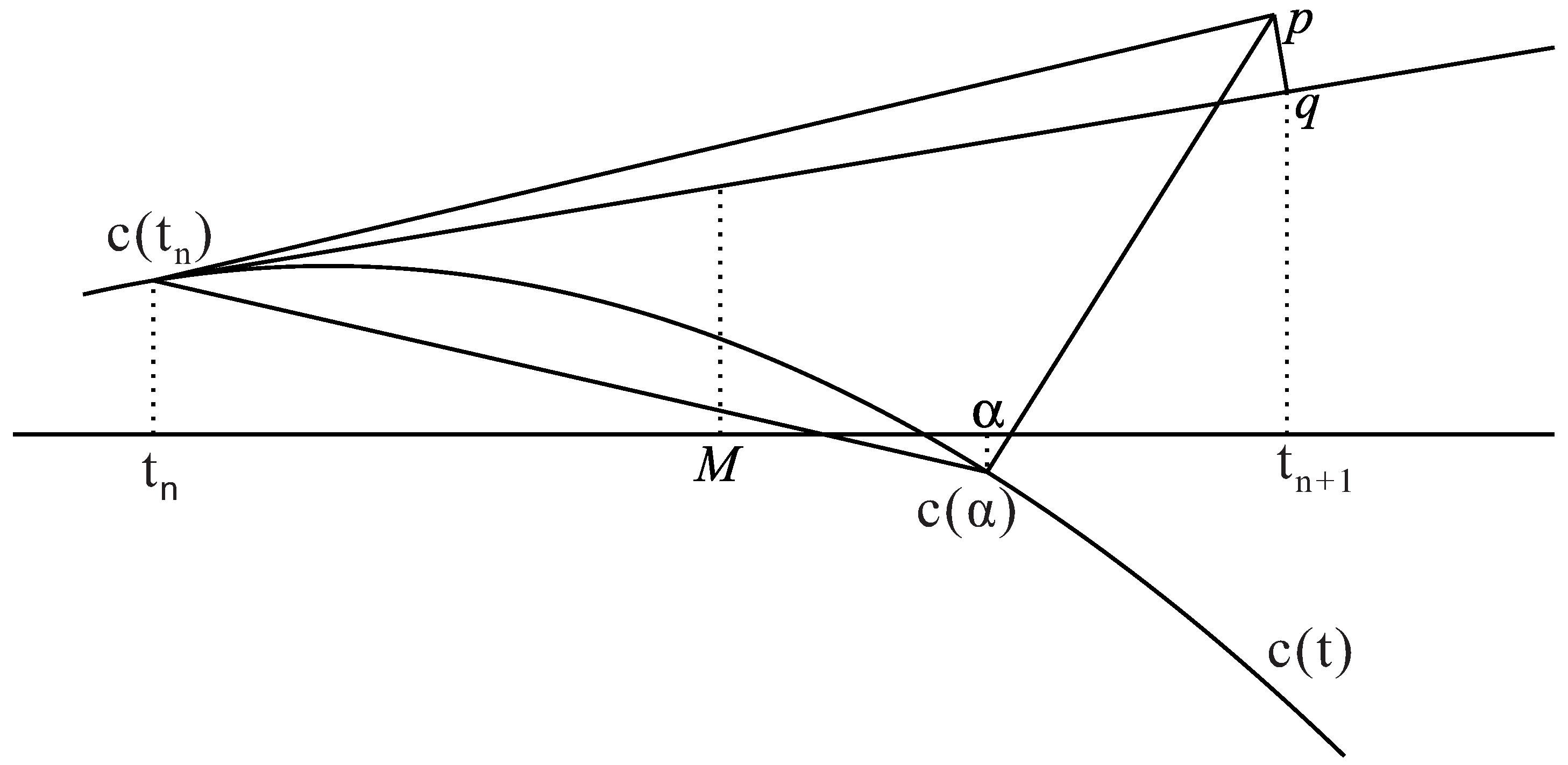
Firstly, we presents the interpretation for Figure 1. Assume there exists a horizontal axis t and planar parametric curve . There are two points on the planar parametric curve : the first point with on the horizontal axis, and the second point is the corresponding orthogonal projection point of the test point p onto the planar parametric curve , where is the corresponding parameter value on the horizontal axis. While, according to the iterative method (2), the line segment determined by point p and point and tangent line of planar parametric curve at are mutually perpendicular. The tangent line of the planar parametric curve through point will determine a footpoint q, which is obtained by orthogonally projecting test point p onto the tangent line of the curve at . The corresponding parametric value of footpoint q on the horizontal axis is obviously the next iterative value used by the iterative method (2). The corresponding parametric value of the middle point of the line segment determined by the point and the footpoint q is M.
Secondly, we present the proof of Theorem 3. When the iterative method (2) only has one solution, it is independent of the initial value for point projection and inversion problem.
The proof method is similar to the ones in references [33,34,35]. It is not difficult to show that the corresponding parameter of the first dimensional for the planar parametric curve on the two-dimensional horizontal plane is t. When the iterative method (2) begins to iterate, as the iterative parameter value satisfies the inequality relationship , by the graphical demonstration, the parameter corresponding to the footpoint q will be . The middle point of point and point is , which implies the relationship . Additionally, because of , there is an inequality relationship . This result sufficiently yields the inequality , namely, there is an iterative error expression , where . If , then the proving method is similar to the case with . Thus, for the planar parametric curve , there is an iterative error expression in the two-dimensional horizontal plane, namely, the iterative method (2) is independent of the initial iterative parametric value.
Alternatively, we will present a descriptive proof that the iterative method (2) is independent of the initial iterative parametric value. This proof method is also similar to the one in the literature [33,34,35]. Suppose that the starting point lies on the left of , then footpoint q will lie on the right to the starting point, and hence will be positive. By the iterative method (2), the iterative sequence is expressed as follows,
where
If , the sequence is strictly monotonically increasing. If , by at most three iterations, the sequence converge to . Notice that this iterative sequence performs like an attenuated pendulum and converges to . Furthermore, when the starting point lies to the right of , the convergence holds in the same way. To summarize, the footpoint q depends on the test point p all the time, rather than on the starting iteration point. So the iterative method (2) is independent of the initial value. The proof is completed. ☐
Remark 1.
The iterative method (2) is independent of the initial value, but it only requires that is , while the methods in the literature [33,34,35] need to satisfy the sufficient conditions for global convergence. In addition, the iterative method (2) fits in with robustness and stabilization in Professor Les A. Piegl’s view [36].
Remark 2.
If of the Equation (5), then . Hence, we calculate the distance between the point on the curve and the test point p, i.e., . At the same time, in order to deal with the possible failure of the projection or inversion, we use the parameter perturbation method and increment the parameter by a small positive constant ε, , so that the iteration can continue. During the iteration process, when the derivative of the curve at becomes zero, the same perturbation approach is applied. Eventually, min becomes the minimum distance between the curve and the test point p.
3. Numerical Experiments
This section provides numerical evidence to compare the behavior of the Newton iterative algorithm and the iterative method (2) discussed above.
Example 1.
We consider the curve with test point and the corresponding parameter of projection point . Table 1 shows the results of Newton iteration and the iterative method (2). The results verify that the iterative method (2) has better convergence and robustness, while the Newton algorithm is dependent on the initial value but is unstable (See Figure 2).
Example 2.
We use the curve with test point and the corresponding parameter of projection point . Table 2 shows the results of Newton iteration and the iterative method (2). The results also verify that the iterative method (2) has better convergence and robustness, while Newton algorithm is dependent on the initial value but is unstable (See Figure 3).
Example 3.
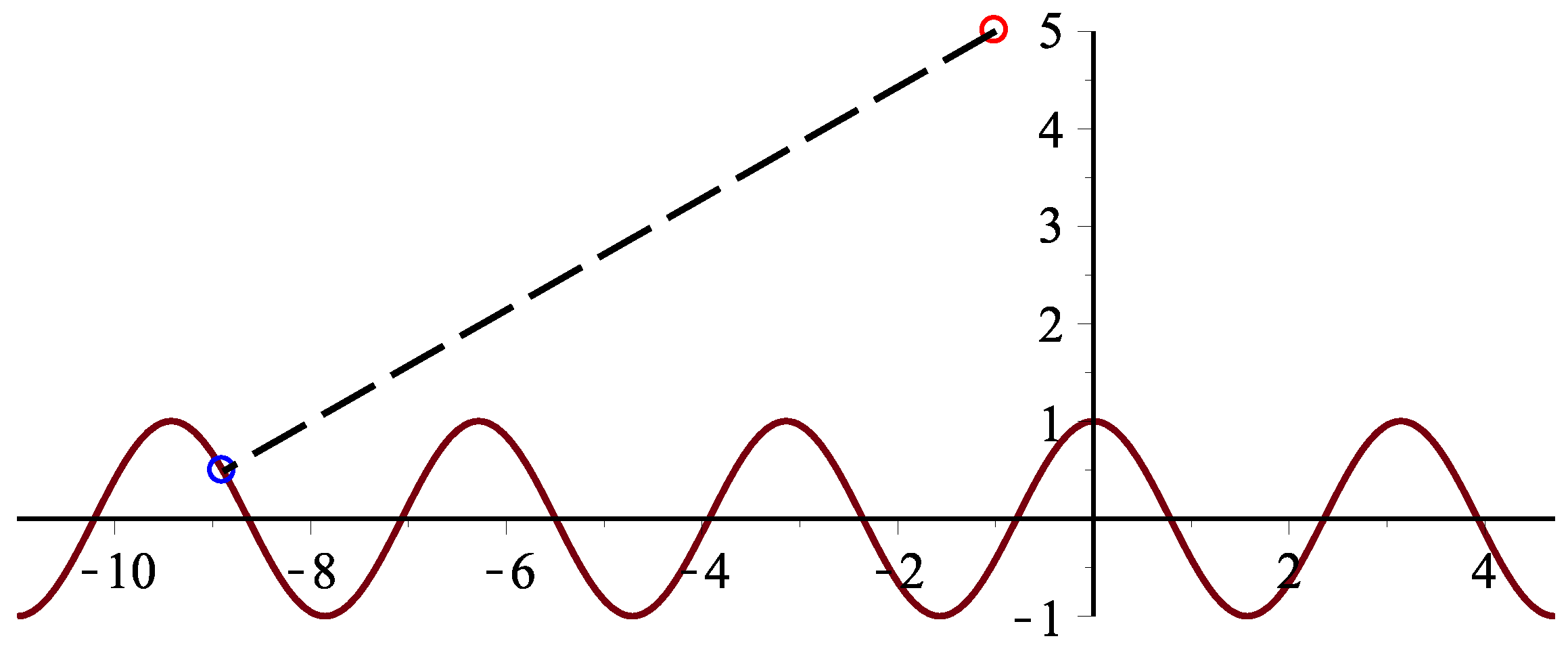
We consider the curve with test point is p and the corresponding parameter of projection point . Table 3 shows the number of iterations for the Newton iteration and the iterative method (2). The results show the iterative method (2) has better convergence and robustness, at the same time, the Newton’s method sometimes converges slowly and depends on the initial value but is unstable (See Figure 4).
Example 4.
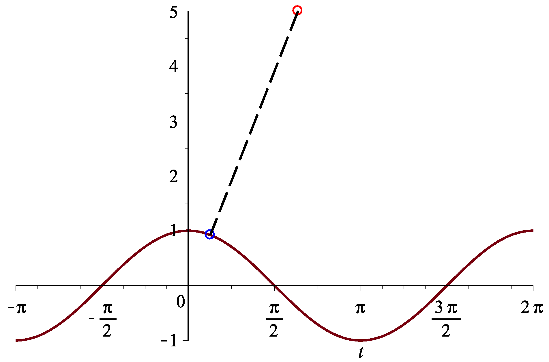
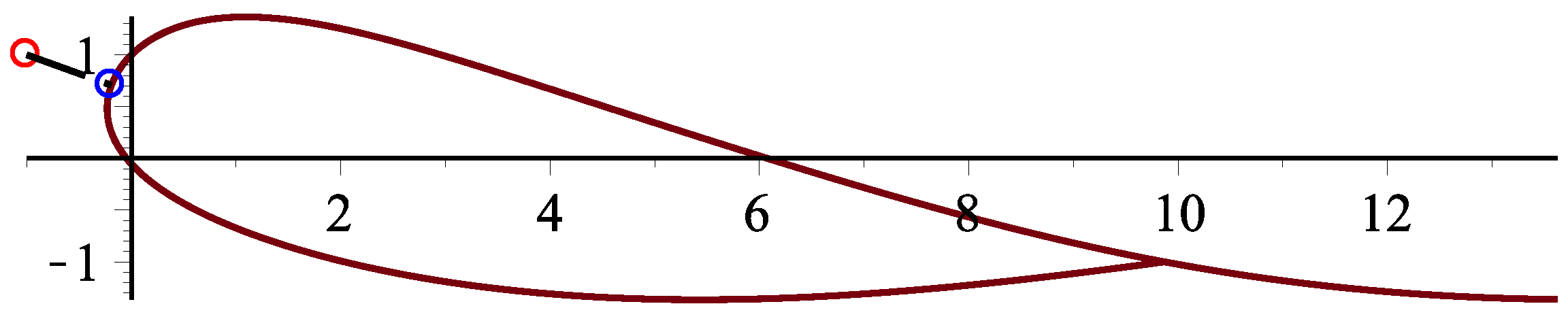
We use the curve . Test point and the corresponding parameter of projection point is . Table 4 shows the number of iterations for Newton iteration and the iterative method (2). Results show the iterative method (2) has better convergence and robustness, at the same time, Newton’s method is sometimes dependent on the initial value but is unstable (See Figure 5).
Example 5.
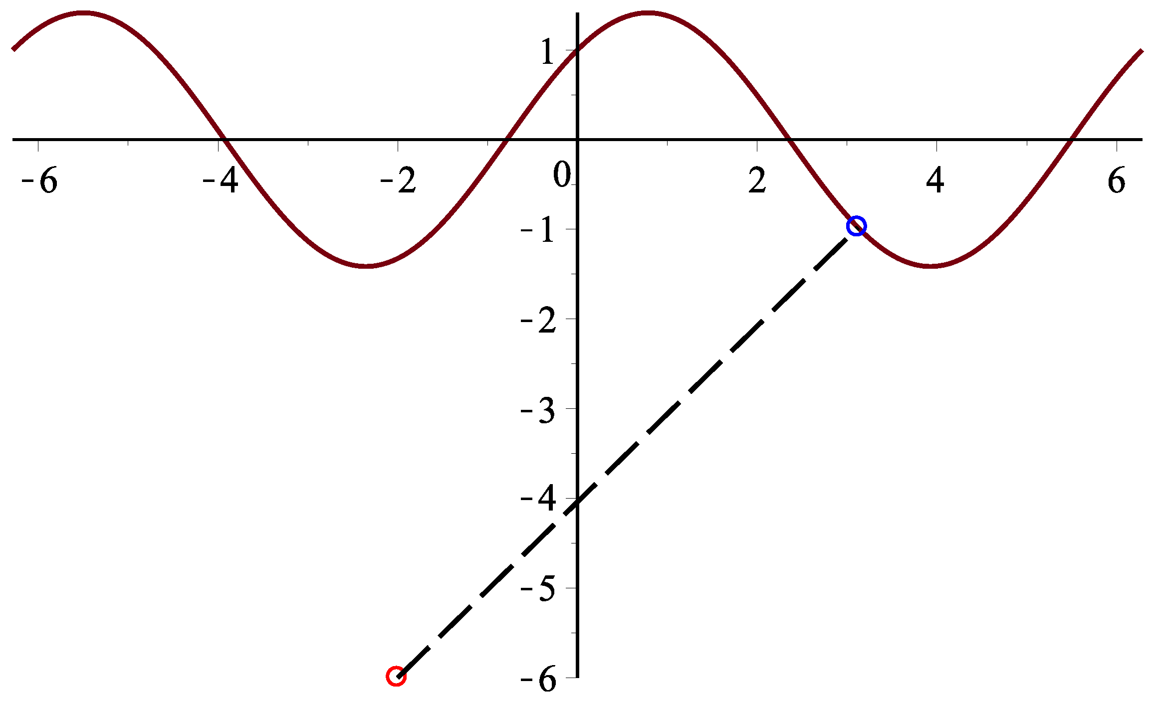
We consider the curve . Test point is , and the corresponding parameter of projection point is . Table 5 shows number of iterations for Newton iteration and the iterative method (2). Results show the the iterative method (2) has better convergence and robustness, at the same time, Newton’s method is sometimes dependent on the initial value but is unstable (See Figure 6).
Example 6.
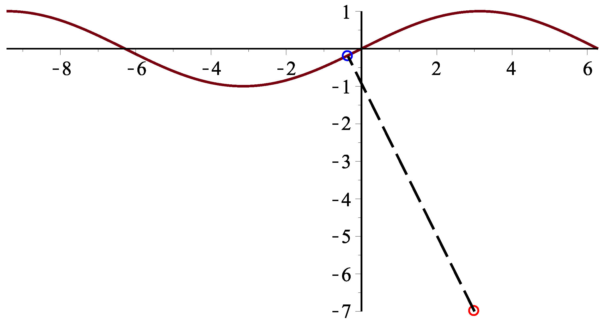
We use the curve . The test point is , and the corresponding parameter of projection point is . Table 6 shows the number of iterations for Newton iteration and the iterative method (2). Results show the iterative method (2) has better convergence and robustness, at the same time, Newton’s method is sometimes dependent on the initial value but is unstable (See Figure 7).
Remark 3.
The iterative method (2) orthogonally projects a test point onto a parametric curve . For the case with multiple orthogonal points, our approach is changed in the following way:
- (1)
- Divide a parameter interval of parametric curve into M subintervals with equal length.
- (2)
- Randomly select an initial iterative parametric value in each subinterval.
- (3)
- Using the iterative method (2) and using each initial iterative parametric value, iterate, respectively. Suppose that the iterative parametric values are , ,…,, respectively.
- (4)
- Calculate the local minimum distances , where .
- (5)
- Calculate the global minimum distance .
If we attempt to search all the solutions as fast as possible, divide a parameter interval into M subintervals with equal length such that M is sufficiently large.
According to Figure 5 and Figure 7, either blue point is the only orthogonal projection point of the test point, but not the point with minimum distance. For in Figure 5, four parameter values are , , , , respectively. According to Remark 3, it is easy to find that the orthogonal projection point determined by the parameter value of −2.3086073340017088 is the one with minimum distance, but the orthogonal projection points determined by the other parameter values are not. For in Figure 7, eight parameter values are , , , , , , , , respectively. In the same way, only the orthogonal projection point determined by the parameter value of is the one with minimum distance.
4. Conclusions
In this paper, regarding the point projection problem, we formally prove that projection of a point onto a planar parameter curve is quadratically convergent and independent of the initial value. On the point inversion problem, we formally prove that the inversion problem is cubically convergent and independent of the initial value. In the future, we would like to present a formal proof of convergence on projecting a point onto a spatial parametric curve and surface in literature [4].
Acknowledgments
We would like to thank the editor and two anonymous reviewers for their efforts to improve greatly the manuscript. We acknowledge the support by the National Natural Science Foundation of China (Grant No. 61263034, Grant No. 71772106), Scientific and Technology Foundation Funded Project of Guizhou Province (Grant No. [2014]2092, Grant No. [2014]2093), Feature Key Laboratory for Regular Institutions of Higher Education of Guizhou Province (Grant No. [2016]003), National Bureau of Statistics Foundation Funded Project (Grant No. 2014LY011), Key Laboratory of Pattern Recognition and Intelligent System of Construction Project of Guizhou Province (Grant No. [2009]4002), Information Processing and Pattern Recognition for Graduate Education Innovation Base of Guizhou Province. Linke Hou is supported by Shandong Provincial Natural Science Foundation of China (Grant No. ZR2016GM24). Juan Liang is supported by Scientific and Technology Key Foundation of Taiyuan Institute of Technology (Grant No. 2016LZ02). Qiaoyang Li is supported by Fund of National Social Science (No. 14XMZ001) and Fund of Chinese Ministry of Education (No. 15JZD034).
Author Contributions
The contributions of all of the authors are the same. All of them have worked together to develop the present manuscript.
Conflicts of Interest
The authors declare no conflict of interest.
References
- Limaiem, A.; Trochu, F. Geometric algorithms for the intersection of curves and surfaces. Comput. Graph. 1995, 19, 391–403. [Google Scholar] [CrossRef]
- Li, X.; Wu, Z.; Hou, L.; Wang, L.; Yue, C.; Xin, Q. A geometric orthogonal projection strategy for computing the minimum distance between a point and a spatial parametric curve. Algorithms 2016, 9, 15. [Google Scholar] [CrossRef]
- Pottmann, H.; Leopoldseder, S.; Hofer, M. Registration without ICP. Comput. Vis. Image Underst. 2004, 95, 54–71. [Google Scholar] [CrossRef]
- Hu, S.M.; Wallner, J. A second order algorithm for orthogonal projection onto curves and surfaces. Comput. Aided Geom. Des. 2005, 22, 251–260. [Google Scholar] [CrossRef]
- Piegl, L.A.; Tiller, W. Parameterization for surface fitting in reverse engineering. Comput. Aided Des. 2001, 33, 593–603. [Google Scholar] [CrossRef]
- Ma, Y.L.; Hewitt, W.T. Point inversion and projection for NURBS curve and surface: Control polygon approach. Comput. Aided Geom. Des. 2000, 20, 79–99. [Google Scholar] [CrossRef]
- Oh, Y.T.; Kim, Y.J.; Lee, J.; Kim, M.S.; Elber, G. Continuous point projection to planar freeform curves using spiral curves. Vis. Comput. 2011, 28, 111–123. [Google Scholar] [CrossRef]
- Srijuntongsiri, G. An iterative/subdivision hybrid algorithm for curve/curve intersection. Vis. Comput. 2011, 27, 365–371. [Google Scholar] [CrossRef]
- Chen, X.D.; Ma, W. Geometric point interpolation method in R3 space with tangent directional constraint. Comput. Aided Des. 2012, 44, 1217–1228. [Google Scholar] [CrossRef]
- Chen, X.D.; Yang, C.; Ma, W. Coincidence condition of two Bézier curves of an arbitrary degree. Comput. Graph. 2016, 54, 121–126. [Google Scholar] [CrossRef]
- Chen, X.D.; Ma, W.; Ye, Y. A rational cubic clipping method for computing real roots of a polynomial. Comput. Aided Geom. Des. 2015, 38, 40–50. [Google Scholar] [CrossRef]
- Chen, X.D.; Ma, W. Rational cubic clipping with linear complexity for computing roots of polynomials. Appl. Math. Comput. 2016, 273, 1051–1058. [Google Scholar] [CrossRef]
- Lin, H.W. Local progressive-iterative approximation format for blending curves and patches. Comput. Aided Geom. Des. 2010, 27, 322–339. [Google Scholar] [CrossRef]
- Lin, H.W. The convergence of the geometric interpolation algorithm. Comput. Aided Des. 2010, 42, 505–508. [Google Scholar] [CrossRef]
- Lin, H.; Qin, Y.; Liao, H.; Xiong, Y. Affine arithmetic-based B-Spline surface intersection with gpu acceleration. IEEE Trans. Vis. Comput. Graph. 2014, 20, 172–181. [Google Scholar] [PubMed]
- Sederberg, T.W.; Lin, H.; Li, X. Curvature of singular Bézier curves and surfaces. Comput. Aided Geom. Des. 2011, 28, 233–244. [Google Scholar] [CrossRef]
- Lin, H.; Zhang, Z. An efficient method for fitting large data sets using T-Splines. SIAM J. Sci. Comput. 2013, 35, A3052–A3068. [Google Scholar] [CrossRef]
- Chen, X.D.; Yong, J.H.; Wang, G.; Paul, J.C.; Xu, G. Computing the minimum distance between a point and a NURBS curve. Comput. Aided Des. 2008, 40, 1051–1054. [Google Scholar] [CrossRef] [Green Version]
- Chen, X.D.; Xu, G.; Yong, J.H.; Wang, G.; Paul, J.C. Computing the minimum distance between a point and a clamped B-spline surface. Graph. Model. 2009, 71, 107–112. [Google Scholar] [CrossRef] [Green Version]
- Chen, X.D.; Ma, W. A planar quadratic clipping method for computing a root of a polynomial in an interval. Comput. Graph. 2015, 46, 89–98. [Google Scholar] [CrossRef]
- Mortenson, M.E. Geometric Modeling; Wiley: New York, NY, USA, 1985; pp. 305–317. [Google Scholar]
- Oh, Y.T.; Kim, Y.J.; Lee, J.; Kim, M.S.; Elber, G. Efficient point-projection to freeform curves and surfaces. Comput. Aided Geom. Des. 2012, 29, 242–254. [Google Scholar] [CrossRef]
- Chen, X.; Zhou, Y.; Shu, Z.; Su, H. Improved Algebraic Algorithm On Point Projection For Bézier Curves. In Proceedings of the Second International Multi-Symposium of Computer and Computational Sciences (IMSCCS 2007), the University of Iowa, Iowa City, IA, USA, 13–15 August 2007. [Google Scholar]
- Song, H.C.; Yong, J.H.; Yang, Y.J.; Liu, X.M. Algorithm for orthogonal projection of parametric curves onto B-spline surfaces. Comput. Aided Des. 2011, 43, 381–393. [Google Scholar] [CrossRef]
- Sundar, B.R.; Chunduru, A.; Tiwari, R.; Gupta, A.; Muthuganapathy, R. Footpoint distance as a measure of distance computation between curves and surfaces. Comput. Graph. 2014, 38, 300–309. [Google Scholar] [CrossRef]
- Wang, X.; Zhang, W.; Huang, X. Computation of point inversion and ray-surface intersection through tracing along the base surface. Vis. Comput. 2015, 31, 1487–1500. [Google Scholar] [CrossRef]
- Li, X.; Wang, L.; Wu, Z.; Hou, L.; Liang, J.; Li, Q. Hybrid second-order iterative algorithm for orthogonal projection onto a parametric surface. Symmetry 2017, 9, 146. [Google Scholar] [CrossRef]
- Li, K.; Sundin, M.; Rojas, C.R.; Chatterjee, S.; Jansson, M. Alternating strategies with internal ADMM for low-rank matrix reconstruction. Signal Process. 2016, 121, 153–159. [Google Scholar] [CrossRef]
- Li, X.; Mu, C.; Ma, J.; Wang, C. Sixteenth-order method for nonlinear equations. Appl. Math. Comput. 2010, 215, 3754–3758. [Google Scholar] [CrossRef]
- Li, X.; Mu, C.; Ma, J.; Hou, L. Fifth-order iterative method for finding multiple roots of nonlinear equations. Numer. Algoritm. 2011, 57, 389–398. [Google Scholar] [CrossRef]
- Li, X.; Xin, Q.; Wu, Z.; Zhang, M.; Zhang, Q. A geometric strategy for computing intersections of two spatial parametric curves. Vis. Comput. 2013, 29, 1151–1158. [Google Scholar] [CrossRef]
- Traub, J.F. Iterative Methods for Solution of Equations; Prentice-Hall: Englewood Cliffs, NJ, USA, 1964. [Google Scholar]
- Melman, A. Geometry and Convergence of Euler’s and Halley’s Methods. SIAM Rev. 1997, 39, 728–735. [Google Scholar] [CrossRef]
- Melman, A. Analysis of third order Methods for Secular Equations. Math. Comput. 1998, 67, 271–286. [Google Scholar] [CrossRef]
- Traub, J.F. A Class of Globally Convergent Iteration Functions for the Solution of Polynomial Equations. Math. Comput. 1966, 20, 113–138. [Google Scholar] [CrossRef]
- Piegl, L.A. Ten challenges in computer-aided design. Comput. Aided Des. 2005, 37, 461–470. [Google Scholar] [CrossRef]
Figure 1.
Graphic demonstration for convergence analysis.

Figure 2.
Graphic demonstration for Example 1.
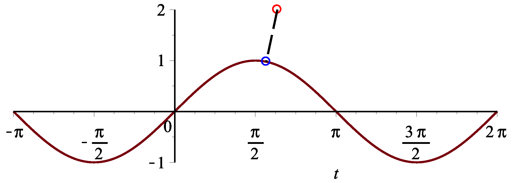
Figure 3.
Graphic demonstration for Example 2.

Figure 4.
Graphic demonstration for Example 3.

Figure 5.
Graphic demonstration for Example 4.

Figure 6.
Graphic demonstration for Example 5.

Figure 7.
Graphic demonstration for Example 6.

Table 1.
Step sizes , in Example 1 for the Newton method and the iterative method (2).
| iterative methods | Step | 1 | 2 | 3 | 4 | 5 | 6 |
| Newton method | NC | NC | NC | NC | NC | NC | |
| The iterative method (2) | 1.82 | 0 | |||||
| iterative methods | Step | 2 | 3 | 4 | 5 | 6 | 7 |
| Newton method | NC | NC | NC | NC | NC | NC | |
| The iterative method (2) | 0 | ||||||
Table 2.
Step sizes , in Example 2 for the Newton method and the iterative method (2).
| , | ||||||||
| iterative methods | Step | 4 | 5 | 6 | 7 | 8 | 9 | 10 |
| Newton method | NC | NC | NC | NC | NC | NC | NC | |
| The iterative method (2) | −1.04 | 0.0 | ||||||
| iterative methods | Step | 5 | 6 | 7 | 8 | 9 | 10 | 11 |
| Newton method | NC | NC | NC | NC | NC | NC | NC | |
| The iterative method (2) | −1.34 | −0.461 | 0 | |||||
Table 3.
Comparison of the robustness and effectiveness for the Newton’s method and the iterative method (2).
Table 3.
Comparison of the robustness and effectiveness for the Newton’s method and the iterative method (2).
| −20 | −16 | −13 | −10 | −7 | −2 | 0 | 1 | 5 | 8 | 11 | 15 | 18 | 20 | |
| The iterative method (2) | 7 | 7 | 7 | 7 | 6 | 5 | 4 | 5 | 6 | 7 | 7 | 7 | 8 | 8 |
| Newton’s method | NC | 11 | 11 | 10 | 10 | 7 | 5 | 6 | 9 | 10 | 11 | 11 | 12 | NC |
Table 4.
Comparison of the robustness and effectiveness for the Newton’s method and the iterative method (2).
Table 4.
Comparison of the robustness and effectiveness for the Newton’s method and the iterative method (2).
| 5.75 | 5.76 | 5.77 | 5.78 | 5.79 | 5.80 | 5.82 | 5.84 | 5.85 | 5.87 | |
| The iterative method (2) | 5 | 5 | 6 | 6 | 6 | 7 | 7 | 7 | 7 | 7 |
| Newton method | NC | NC | NC | NC | NC | NC | NC | NC | NC | NC |
| 5.88 | 5.89 | 5.90 | 5.92 | 5.93 | 5.95 | 5.96 | 5.97 | 5.99 | 6.00 | |
| The iterative method (2) | 7 | 6 | 6 | 8 | 10 | 25 | 23 | 24 | 21 | 22 |
| Newton method | NC | NC | NC | NC | NC | NC | NC | NC | NC | NC |
Table 5.
Comparison of the robustness and effectiveness for the Newton’s method and the iterative method (2).
Table 5.
Comparison of the robustness and effectiveness for the Newton’s method and the iterative method (2).
| −5.6 | −5.5 | −5.3 | −5.2 | −5.0 | −4.9 | −4.8 | −4.7 | −4.6 | −4.5 | |
| The iterative method (2) | 11 | 11 | 11 | 12 | 14 | 11 | 13 | 14 | 11 | 14 |
| Newton method | NC | NC | NC | NC | NC | NC | NC | NC | NC | NC |
| −4.3 | −4.0 | −3.8 | −3.4 | −3.0 | −2.3 | −2.0 | −1.0 | 0.4 | 1.0 | |
| The iterative method (2) | 13 | 11 | 16 | 7 | 10 | 6 | 11 | 11 | 12 | 14 |
| Newton method | NC | NC | NC | NC | NC | NC | NC | NC | NC | NC |
Table 6.
Comparison of the robustness and effectiveness for the Newton’s method and the iterative method (2).
Table 6.
Comparison of the robustness and effectiveness for the Newton’s method and the iterative method (2).
| −12.8 | −12.4 | −12.1 | −11.9 | −11.7 | −11.0 | −10.8 | −10.7 | −10.4 | −10.0 | |
| The iterative method (2) | 59 | 55 | 59 | 46 | 46 | 53 | 41 | 42 | 39 | 32 |
| Newton method | NC | NC | NC | NC | NC | NC | NC | NC | NC | NC |
© 2017 by the authors. Licensee MDPI, Basel, Switzerland. This article is an open access article distributed under the terms and conditions of the Creative Commons Attribution (CC BY) license (http://creativecommons.org/licenses/by/4.0/).
Share and Cite
MDPI and ACS Style
Li, X.; Wang, L.; Wu, Z.; Hou, L.; Liang, J.; Li, Q. Convergence Analysis on a Second Order Algorithm for Orthogonal Projection onto Curves. Symmetry 2017, 9, 210. https://doi.org/10.3390/sym9100210
AMA Style
Li X, Wang L, Wu Z, Hou L, Liang J, Li Q. Convergence Analysis on a Second Order Algorithm for Orthogonal Projection onto Curves. Symmetry. 2017; 9(10):210. https://doi.org/10.3390/sym9100210
Chicago/Turabian StyleLi, Xiaowu, Lin Wang, Zhinan Wu, Linke Hou, Juan Liang, and Qiaoyang Li. 2017. "Convergence Analysis on a Second Order Algorithm for Orthogonal Projection onto Curves" Symmetry 9, no. 10: 210. https://doi.org/10.3390/sym9100210
Note that from the first issue of 2016, this journal uses article numbers instead of page numbers. See further details here.