Exact Finite Differences. The Derivative on Non Uniformly Spaced Partitions

Abstract

We define a finite-differences derivative operation, on a non uniformly spaced partition, which has the exponential function as an exact eigenvector. We discuss some properties of this operator and we propose a definition for the components of a finite-differences momentum operator. This allows us to perform exact discrete calculations.

1. Introduction

Early works on discrete quantum mechanics [1,2,3,4,5,6] only consider discrete, uniform jumps along some variable and along its conjugate direction. However, a question is if it is possible to perform continuous translations along the conjugate variable instead of periodic discrete jumps. A previous paper answers this question for systems with a uniform spacing between a mesh of points representing a variable [7], but it would also be very useful to develop the theory for non-uniform mesh points. After all, very few energy spectra have uniformly separated points.

In this paper, we focus on realizing continuous translations on discrete systems with non uniform separation between the discrete values of a given variable, which we will call the coordinate variable.

The results in this paper help to solve a paradox pointed out by Pauli in 1926 [8,9]. We begin by introducing a first-order finite-differences definition of a derivative operator acting on vectors on a non-uniform mesh. Our definition is based on a simple equality and is characterized by having the exponential function as an exact eigenfunction. This is done in Section 2.

In Section 3, we find expressions for higher order derivatives in such a way that the exponential function is still an exact eigenfunction of them all. Some properties of the finite-differences derivative and a summation by parts theorem are the subjects of Section 4.

The eigenvalues and eigenfunctions of the matrix formed with the expressions for the derivative are found in Section 5. These eigenvalues and eigenfunctions are consistent with the corresponding ones for the continuous variable case. The commutator between the coordinate and derivative matrices is the subject of Section 6.

At the end there is a discussion about the use of the results in this paper to propose a definition for finite-differences components of self-adjoint operators.

2. Exact, First-Order, Finite-Differences Derivative

We will consider a mesh $\mathcal{M}\left(N\right):={\left\{q_i\right\}}_1^N$ of N non equally spaced points $q_i$ on the finite interval $[a,b]\in \mathbb{R}$, $a<b<\infty$, with separations ${\Delta }_j=q_{j+1}-q_j$ between them.

An equality is:

$$\begin{array}{c}\hfill e^{v{q}_{j+1}}-e^{v{q}_j}=e^{v{q}_j}(e^{v(q_{j+1}-q_j)}-1),\end{array}$$

(1)

where $v\in \mathbb{C}$. This equality can be rewritten as:

$$\begin{array}{c}\hfill \frac{e^{v{q}_{j+1}}-e^{v{q}_j}}{{\chi }_1(v,j)}=\frac{v}{e^{v{\Delta }_j}-1}(e^{v{q}_{j+1}}-e^{v{q}_j})=v{e}^{v{q}_j},\end{array}$$

(2)

where ${\chi }_1(v,j)=(e^{v{\Delta }_j}-1)/v\approx {\Delta }_j+v{\Delta }_j^2/2+\dots$. This equation suggests that we can define a forward finite differences derivative at $q_j$ as:

$${\left({\mathrm{D}}_{f}g\right)}_j:=\frac{g_{j+1}-g_j}{{\chi }_1(v,j)},$$

(3)

where $g\in \mathbb{C}$ is any bounded complex function evaluated at the points of $\mathcal{M}\left(N\right)$. Similarly, the backward finite-differences derivative of g at $q_j$ is defined as:

$${\left({\mathrm{D}}_{b}g\right)}_j:=\frac{g_j-g_{j-1}}{{\chi }_2(v,j-1)},$$

(4)

where ${\chi }_2(v,j)=(1-e^{-v{\Delta }_j})/v\approx {\Delta }_j-v{\Delta }_j^2/2+\dots$

For small ${\Delta }_j$, the definitions (3) and (4) take the usual forms:

$$\begin{array}{c}\hfill {\left({\mathrm{D}}_{b}g\right)}_j\approx \frac{g_j-g_{j-1}}{{\Delta }_{j-1}},\mathrm{and}{\left({\mathrm{D}}_{f}g\right)}_j\approx \frac{g_{j+1}-g_j}{{\Delta }_j}.\end{array}$$

(5)

The nice property of these finite-differences operators is that the exponential function is an exact eigenvector of them. We will discuss some additional properties of these operators in the next sections.

3. Higher Order Derivatives

The derivatives, (3) and (4), for the whole mesh $\mathcal{M}\left(N\right)$, can be represented with the help of $N\times N$ matrices. For the backward finite differences derivative we propose:

$$\begin{array}{c}\hfill {\mathbf{D}}_b:=\left(\begin{array}{cccccccc}\frac{-1}{{\chi }_1(v,1)}& \frac{1}{{\chi }_1(v,1)}& 0& 0& \dots & 0& 0& 0\\ \frac{-1}{{\chi }_2(v,1)}& \frac{1}{{\chi }_2(v,1)}& 0& 0& \dots & 0& 0& 0\\ 0& \frac{-1}{{\chi }_2(v,2)}& \frac{1}{{\chi }_2(v,2)}& 0& \dots & 0& 0& 0\\ 0& 0& \frac{-1}{{\chi }_2(v,3)}& \frac{1}{{\chi }_2(v,3)}& \dots & 0& 0& 0\\ ⋮\\ 0& 0& 0& 0& \dots & \frac{-1}{{\chi }_2(v,N-2)}& \frac{1}{{\chi }_2(v,N-2)}& 0\\ 0& 0& 0& 0& \dots & 0& \frac{-1}{{\chi }_2(v,N-1)}& \frac{1}{{\chi }_2(v,N-1)}\end{array}\right).\end{array}$$

(6)

Note that we have used a forward derivative at the first mesh point so that we can have a square matrix. The forward finite-differences derivative is associated with the matrix.

$$\begin{array}{c}\hfill {\mathbf{D}}_f:=\left(\begin{array}{cccccccc}\frac{-1}{{\chi }_1(v,1)}& \frac{1}{{\chi }_1(v,1)}& 0& 0& \dots & 0& 0& 0\\ 0& \frac{-1}{{\chi }_1(v,2)}& \frac{1}{{\chi }_1(v,2)}& 0& \dots & 0& 0& 0\\ 0& 0& \frac{-1}{{\chi }_1(v,3)}& \frac{1}{{\chi }_1(v,3)}& \dots & 0& 0& 0\\ ⋮\\ 0& 0& 0& 0& \dots & \frac{-1}{{\chi }_1(v,N-2)}& \frac{1}{{\chi }_1(v,N-2)}& 0\\ 0& 0& 0& 0& \dots & 0& \frac{-1}{{\chi }_1(v,N-1)}& \frac{1}{{\chi }_1(v,N-1)}\\ 0& 0& 0& 0& \dots & 0& \frac{-1}{{\chi }_2(v,N-1)}& \frac{1}{{\chi }_2(v,N-1)}\end{array}\right).\end{array}$$

(7)

This time, we have used a backward derivative at the last point. These are matrices that act on complex vectors $\mathbf{g}={(g_1,g_2,\dots ,g_N)}^T$ on the mesh.

By computing the matrices ${\mathbf{D}}_{b,f}^2$, we obtain expressions for second derivatives at each of the mesh points. For instance, expressions for the second derivative are:

$$\begin{array}{cc}\hfill {\left({\mathrm{D}}_b^{2}g\right)}_1& =v\frac{g_2-g_1}{{\chi }_1(v,1)}=v{\left({\mathrm{D}}_{f}g\right)}_1,\hfill \end{array}$$

(8)

$$\begin{array}{c}\hfill {\left({\mathrm{D}}_b^{2}g\right)}_2=v\frac{g_2-g_1}{{\chi }_2(v,1)}=v{\left({\mathrm{D}}_{b}g\right)}_2,\end{array}$$

(9)

$$\begin{array}{c}\hfill {\left({\mathrm{D}}_b^{2}g\right)}_j=\frac{1}{{\chi }_2(v,j-1)}\left(\frac{g_j-g_{j-1}}{{\chi }_2(v,j-1)}-\frac{g_{j-1}-g_{j-2}}{{\chi }_2(v,j-2)}\right)=\frac{{\left({\mathrm{D}}_{b}g\right)}_j-{\left({\mathrm{D}}_{b}g\right)}_{j-1}}{{\chi }_2(v,j-1)},\end{array}$$

(10)

where $j=3,\dots ,N$.

Expressions for the third derivatives are:

$$\begin{array}{c}\hfill {\left({\mathrm{D}}_b^{3}g\right)}_1=v^2\frac{g_2-g_1}{{\chi }_1(v,1)}=v^2{\left({\mathrm{D}}_{f}g\right)}_1,\end{array}$$

(11)

$$\begin{array}{c}\hfill {\left({\mathrm{D}}_b^{3}g\right)}_2=v^2\frac{g_2-g_1}{{\chi }_2(v,1)}=v^2{\left({\mathrm{D}}_{b}g\right)}_2,\end{array}$$

(12)

$$\begin{array}{cc}\hfill {\left({\mathrm{D}}_b^{3}g\right)}_3& =\frac{1}{{\chi }_2(v,2)}\left[\frac{g_3-g_2}{{\chi }_2^2(v,2)}-\left(\frac{1}{{\chi }_2(v,2)}+v\right)\frac{g_2-g_1}{{\chi }_2(v,1)}\right]\hfill \\ & =\frac{{\left({\mathrm{D}}_{b}g\right)}_3-{\left({\mathrm{D}}_{b}g\right)}_2}{{\chi }_2^2(v,2)}-v\frac{{\left({\mathrm{D}}_{b}g\right)}_2}{{\chi }_2(v,2)}\hfill \\ & =\frac{{\left({\mathrm{D}}_b^{2}g\right)}_3-{\left({\mathrm{D}}_b^{2}g\right)}_2}{{\chi }_2(v,2)},\hfill \end{array}$$

(13)

and

$$\begin{array}{c}{\left({\mathrm{D}}_b^{3}g\right)}_j\hfill \\ =\frac{1}{{\chi }_2(v,j-1)}\left[\frac{g_j}{{\chi }_2^2(v,j-1)}\right.-\left(\frac{1}{{\chi }_2^2(v,j-1)}+\frac{1}{{\chi }_2(v,j-2){\chi }_2(v,j-1)}+\frac{1}{{\chi }_2^2(v,j-2)}\right)g_{j-1}\hfill \\ +\left(\frac{1}{{\chi }_2(v,j-3)}+\frac{1}{{\chi }_2(v,j-2)}+\frac{1}{{\chi }_2(v,j-1)}\right)\frac{g_{j-2}}{{\chi }_2(v,j-2)}\hfill \\ \left.-\frac{g_{j-3}}{{\chi }_2(v,j-3){\chi }_2(v,j-2)}\right]\hfill \\ =\frac{1}{{\chi }_2(v,j-1)}\left[\frac{{\left({\mathrm{D}}_{b}g\right)}_{j-2}}{{\chi }_2(v,j-2)}-\left(\frac{1}{{\chi }_2(v,j-1)}+\frac{1}{{\chi }_2(v,j-2)}\right){\left({\mathrm{D}}_{b}g\right)}_{j-1}\right.\hfill \\ \left.+\frac{{\left({\mathrm{D}}_{b}g\right)}_j}{{\chi }_2(v,j-1)}\right]\hfill \\ =\frac{{\left({\mathrm{D}}_b^{2}g\right)}_j-{\left({\mathrm{D}}_b^{2}g\right)}_{j-1}}{{\chi }_2(v,j-1)},\hfill \end{array}$$

(14)

where $4\le j\le N$. These results provide expressions for backward finite-differences third order derivatives for all the points of the mesh in such a way that the exponential function is still one of its eigenfunctions.

Similar expressions for the forward finite-differences derivatives can be obtained.

4. Summation by Parts Theorem

An important result for continuous functions is the integration by parts theorem. We will look for the discrete version of that theorem but we need some previous results.

The derivative matrices ${\mathbf{D}}_{b,f}$ are singular and they do not have an inverse. However, the inverse operation to the first order finite-differences derivatives D${}_{b,f}$ at some mesh point is the summation with weights ${\chi }_1(v,j)$ or ${\chi }_2(v,j)$. For integers $m,n$ we have:

$$\begin{array}{c}\hfill \sum _{j=n}^m{\chi }_1(v,j){\left({\mathrm{D}}_{f}g\right)}_j=\sum _{j=n}^m(g_{j+1}-g_j)=g_{m+1}-g_n,\end{array}$$

(15)

where $1\le n<m<N$ and

$$\begin{array}{c}\hfill \sum _{j=n}^m{\chi }_2(v,j-1){\left({\mathrm{D}}_{b}g\right)}_j=g_m-g_{n-1},\end{array}$$

(16)

where $1<n<m\le N$.

The usual integral of the exponential function is also obtainable as a finite-differences equality. According to (15) and (16), we have:

$$\begin{array}{cc}\hfill \sum _{j=n}^m{\chi }_1(v,j)v{e}^{v{q}_j}& =\sum _{j=n}^m{\chi }_1(v,j){\left({\mathrm{D}}_f{e}^{vq}\right)}_j=e^{v{q}_{m+1}}-e^{v{q}_n},\hfill \end{array}$$

(17)

where $1\le n<m<N$, and

$$\begin{array}{c}\hfill \sum _{j=n}^m{\chi }_2(v,j-1)v{e}^{v{q}_j}=e^{v{q}_m}-e^{v{q}_{n-1}},\end{array}$$

(18)

where $1<n<m\le N$.

The finite-differences version of the chain rule is:

$$\begin{array}{cc}\hfill {\left({\mathrm{D}}_{f}g\left(h\left(q\right)\right)\right)}_j& =\frac{g\left(h\left(q_{j+1}\right)\right)-g\left(h\left(q_j\right)\right)}{{\chi }_1(v,j)}=v\frac{g\left(h\left(q_{j+1}\right)\right)-g\left(h\left(q_j\right)\right)}{e^{v(h\left(q_{j+1}\right)-h\left(q_j\right))}-1}\frac{e^{v(h\left(q_{j+1}\right)-h\left(q_j\right))}-1}{v{\chi }_1(v,j)}\hfill \\ & ={\left({\mathrm{D}}_{f}g\right)}_j\frac{{\chi }_1(v,{\Delta }_{h,j})}{{\chi }_1(v,j)},\hfill \end{array}$$

(19)

where

$${\left({\mathrm{D}}_{f}g\right)}_j:=v\frac{g\left(h\left(q_{j+1}\right)\right)-g\left(h\left(q_j\right)\right)}{e^{v(h\left(q_{j+1}\right)-h\left(q_j\right))}-1}$$

(20)

${\chi }_1(v,{\Delta }_{h,j})=(e^{v(h\left(q_{j+1}\right)-h\left(q_j\right))}-1)/v$ and ${\Delta }_{h,j}=h\left(q_{j+1}\right)-h\left(q_j\right)$. Also

$$\begin{array}{c}\hfill {\left({\mathrm{D}}_{b}g\left(h\left(q\right)\right)\right)}_j={\left({\mathrm{D}}_{b}g\right)}_j\frac{{\chi }_2(v,{\Delta }_{h,j-1})}{{\chi }_2(v,j-1)},\end{array}$$

(21)

where ${\chi }_2(v,{\Delta }_{h,j-1})=(1-e^{-v(h\left(q_j\right)-h\left(q_{j-1}\right))})/v$, and

$${\left({\mathrm{D}}_{b}g\right)}_j:=v\frac{g\left(h\left(q_j\right)\right)-g\left(h\left(q_{j-1}\right)\right)}{1-e^{-v(h\left(q_j\right)-h\left(q_{j-1}\right))}}.$$

(22)

Now, the exact finite-differences derivative of a product is:

$$\begin{array}{cc}\hfill {\left({\mathrm{D}}_{f}gh\right)}_j& =\frac{g_{j+1}{h}_{j+1}-g_j{h}_j}{{\chi }_1(v,j)}=g_{j+1}\frac{h_{j+1}-h_j}{{\chi }_1(v,j)}+\frac{g_{j+1}-g_j}{{\chi }_1(v,j)}{h}_j=g_{j+1}{\left({\mathrm{D}}_{f}h\right)}_j+h_j{\left({\mathrm{D}}_{f}g\right)}_j\hfill \\ & =e^{-v{\Delta }_j}{g}_{j+1}{\left({\mathrm{D}}_{b}h\right)}_{j+1}+h_j{\left({\mathrm{D}}_{f}g\right)}_j,\hfill \end{array}$$

(23)

where $1\le j<N$ and $h\left(q\right)$ is any bounded complex function on $[a,b]$. Also

$$\begin{array}{c}\hfill {\left({\mathrm{D}}_{b}gh\right)}_j=g_j{\left({\mathrm{D}}_{b}h\right)}_j+h_{j-1}{\left({\mathrm{D}}_{b}g\right)}_j=g_j{\left({\mathrm{D}}_{b}h\right)}_j+e^{v{\Delta }_{j-1}}{h}_{j-1}{\left({\mathrm{D}}_{f}g\right)}_{j-1},\end{array}$$

(24)

where $1<j\le N$.

For the finite differences derivative of the ratio of two functions we have:

$$\begin{array}{cc}\hfill {\left({\mathrm{D}}_b\frac{g}{h}\right)}_j& =\frac{1}{{\chi }_2(v,j-1)}\left(\frac{g_j}{h_j}-\frac{g_{j-1}}{h_{j-1}}\right)=\frac{1}{{\chi }_2(v,j-1)}\left(-\frac{g_j(h_j-h_{j-1})}{h_j{h}_{j-1}}+\frac{(g_j-g_{j-1})h_j}{h_j{h}_{j-1}}\right)\hfill \\ & =\frac{{\left({\mathrm{D}}_{b}g\right)}_j}{h_{j-1}}-g_j\frac{{\left({\mathrm{D}}_{b}h\right)}_j}{h_j{h}_{j-1}},\hfill \end{array}$$

(25)

$$\begin{array}{c}\hfill {\left({\mathrm{D}}_b\frac{g}{h}\right)}_j=\frac{{\left({\mathrm{D}}_{b}g\right)}_j}{h_j}-g_{j-1}\frac{{\left({\mathrm{D}}_{b}h\right)}_j}{h_{j-1}{h}_j},\end{array}$$

(26)

$$\begin{array}{c}\hfill {\left({\mathrm{D}}_f\frac{g}{h}\right)}_j=\frac{{\left({\mathrm{D}}_{f}g\right)}_j}{h_{j+1}}-g_j\frac{{\left({\mathrm{D}}_{f}h\right)}_j}{h_j{h}_{j+1}},\end{array}$$

(27)

$$\begin{array}{c}\hfill {\left({\mathrm{D}}_f\frac{g}{h}\right)}_j=\frac{{\left({\mathrm{D}}_{f}g\right)}_j}{h_j}-g_{j+1}\frac{{\left({\mathrm{D}}_{f}h\right)}_j}{h_j{h}_{j+1}}.\end{array}$$

(28)

A couple of equalities that will be needed below are:

$$\begin{array}{c}\hfill \frac{1}{{\chi }_2(v,j)}-\frac{1}{{\chi }_1(v,j)}=v,\mathrm{and}\frac{{\chi }_1(v,j)}{{\chi }_2(v,j)}=e^{v{\Delta }_j}.\end{array}$$

(29)

Thus, the sum of equalities (23) and (24) will provide the exact finite-differences summation by parts theorems,

$$\begin{array}{c}\sum _{j=n}^m{\chi }_2(v,j)g_{j+1}{\left({\mathrm{D}}_{b}h\right)}_{j+1}+\sum _{j=n}^m{\chi }_1(v,j)h_j{\left({\mathrm{D}}_{f}g\right)}_j=g_{m+1}{h}_{m+1}-g_n{h}_n,\hfill \end{array}$$

(30)

where $1\le j<N$, and

$$\begin{array}{c}\sum _{j=n}^m{\chi }_2(v,j-1)g_j{\left({\mathrm{D}}_{b}h\right)}_j+\sum _{j=n}^m{\chi }_1(v,j-1)h_{j-1}{\left({\mathrm{D}}_{f}g\right)}_{j-1}=g_m{h}_m-g_{n-1}{h}_{n-1},\hfill \end{array}$$

(31)

where $1<j\le N$.

5. Eigenvalues and Eigenvectors

The eigenvalues of the matrix ${\mathbf{D}}_f$ are given as the solution to the equation:

$$\begin{array}{c}\left|\begin{array}{cccccc}\frac{-1}{{\chi }_1\left(1\right)}-\lambda & \frac{1}{{\chi }_1\left(1\right)}& 0& \dots & 0& 0\\ 0& \frac{-1}{{\chi }_1\left(2\right)}-\lambda & \frac{1}{{\chi }_1\left(2\right)}& \dots & 0& 0\\ 0& 0& \frac{-1}{{\chi }_1\left(3\right)}-\lambda & \dots & 0& 0\\ ⋮\\ 0& 0& 0& \dots & \frac{1}{{\chi }_1(N-2)}& 0\\ 0& 0& 0& \dots & \frac{-1}{{\chi }_1(N-1)}-\lambda & \frac{1}{{\chi }_1(N-1)}\\ 0& 0& 0& \dots & \frac{-1}{{\chi }_2(N-1)}& \frac{1}{{\chi }_2(N-1)}-\lambda \end{array}\right|\hfill \\ =\lambda (\lambda -v)\left(\frac{-1}{{\chi }_1(v,1)}-\lambda \right)\left(\frac{-1}{{\chi }_1(v,2)}-\lambda \right)\cdots \left(\frac{-1}{{\chi }_1(v,N-2)}-\lambda \right)\hfill \\ =0,\hfill \end{array}$$

(32)

i.e., there is an eigenvalue $\lambda =0$, $N-2$ eigenvalues $\lambda =-1/{\chi }_1(v,j)$, $j=1,\dots ,N-2$, and $\lambda =v$.

When the eigenvalue is zero, we have the following simultaneous system of equations for the components of the eigenvector denoted by ${\mathbf{e}}_0={(e_{0,1},e_{0,2},\dots ,e_{0,N})}^T$

$$\frac{e_{0,j}-e_{0,j-1}}{{\chi }_2(v,j-1)}=0,j=2,\dots ,N,$$

(33)

with solution

$${\mathbf{e}}_0=\frac{1}{\sqrt{N}}{(1,1,1,\dots ,1)}^T.$$

(34)

The eigenvalue $\lambda =-1/{\chi }_1(v,{\Delta }_j)$ gives rise to the following set of equations for the components of the eigenvector, denoted by ${\mathbf{e}}_{j+1}$, $j=1,2,\dots ,N-2$,

$$\begin{array}{cc}\hfill \left(\frac{-1}{{\chi }_1(v,1)}+\frac{1}{{\chi }_1(v,j)}\right)e_{j+1,1}+\frac{e_{j+1,2}}{{\chi }_1(v,1)}& =0,\hfill \end{array}$$

(35)

$$\begin{array}{cc}\hfill \left(\frac{-1}{{\chi }_1(v,2)}+\frac{1}{{\chi }_1(v,j)}\right)e_{j+1,2}+\frac{e_{j+1,3}}{{\chi }_1(v,2)}& =0,\hfill \\ \hfill ⋮& \end{array}$$

(36)

$$\begin{array}{cc}\hfill \left(\frac{-1}{{\chi }_1(v,j-1)}+\frac{1}{{\chi }_1(v,j)}\right)e_{j+1,j-1}+\frac{e_{j+1,j}}{{\chi }_1(v,j-1)}& =0,\hfill \end{array}$$

(37)

$$\begin{array}{cc}\hfill \left(\frac{-1}{{\chi }_1(v,j)}+\frac{1}{{\chi }_1(v,j)}\right)e_{j+1,j}+\frac{e_{j+1,j+1}}{{\chi }_1(v,j)}& =0,\hfill \end{array}$$

(38)

$$\begin{array}{cc}\hfill \left(\frac{-1}{{\chi }_1(v,j+1)}+\frac{1}{{\chi }_1(v,j)}\right)e_{j+1,j+1}+\frac{e_{j+1,j+2}}{{\chi }_1(v,j+1)}& =0,\hfill \\ \hfill ⋮& \end{array}$$

(39)

$$\begin{array}{cc}\hfill \left(\frac{-1}{{\chi }_1(v,N-2)}+\frac{1}{{\chi }_1(v,j)}\right)e_{j+1,N-2}+\frac{e_{j+1,N-1}}{{\chi }_1(v,N-2)}& =0,\hfill \end{array}$$

(40)

$$\begin{array}{cc}\hfill \left(\frac{-1}{{\chi }_1(v,N-1)}+\frac{1}{{\chi }_1(v,j)}\right)e_{j+1,N-1}+\frac{e_{j+1,N}}{{\chi }_1(v,N-1)}& =0,\hfill \end{array}$$

(41)

$$\begin{array}{cc}\hfill \left(\frac{-1}{{\chi }_2(v,N-1)}+\frac{1}{{\chi }_1(v,j)}\right)e_{j+1,N-1}+\frac{e_{j+1,N}}{{\chi }_2(v,N-1)}& =0,\hfill \end{array}$$

(42)

with solution

$$\begin{array}{cc}\hfill \left(1-\frac{{\chi }_1(v,m)}{{\chi }_1(v,j)}\right)e_{j+1,m}& =e_{j+1,m+1},m=1,\dots ,j-1\hfill \end{array}$$

(43)

$$\begin{array}{cc}\hfill e_{j+1,m}& =0,m=j+1,\dots ,N.\hfill \end{array}$$

(44)

These are approximately the vectors ${(1,0,\dots ,0)}^T$ and the null vector when $e_{j+1,1}=0$. The components of the eigenvector fluctuate in the first components; if the values of ${\chi }_1(v,j)$ are similar, the left hand side of these equalities are close to vanish, and they actually vanish for an equally spaced partition.

More interestingly, the eigenvector corresponding to the eigenvalue v is an exponential function, i.e.,

$${\mathbf{e}}_v:={(e^{v(q_1-q_0)},e^{v(q_2-q_0)},e^{v(q_3-q_0)},\dots ,e^{v(q_{N-1}-q_0)},e^{v(q_N-q_0)})}^T,$$

(45)

where $q_0$ is an arbitrary constant. This is the exponential function evaluated at the mesh points $\left\{q_i\right\}$ relative to the arbitrary $q_0$.

Because the exponential function is one of the eigenvectors of the derivative matrix, we can say that:

$$\begin{array}{cc}\hfill e^{u{\mathbf{D}}_f}{\mathbf{e}}_v& =\sum _{n=0}^{\infty }\frac{1}{n!}{\left(u{\mathbf{D}}_f\right)}^n{\mathbf{e}}_v=\sum _{n=0}^{\infty }\frac{1}{n!}{\left(vu\right)}^n{\mathbf{e}}_v=e^{vu}{\mathbf{e}}_v\hfill \\ & ={(e^{v(u+q_1-q_0)},e^{v(u+q_2-q_0)},\dots ,e^{v(u+q_{N-1}-q_0)},e^{v(u+q_N-q_0)})}^T,\hfill \end{array}$$

(46)

which is a translation of the eigenvector ${\mathbf{e}}_v$ by an amount u along the coordinate direction. This can be seen as having the same function but now the domain has changed, it was translated by the amount u and the function is now evaluated at the new points of the domain, a continuous translation [10].

6. The Commutator

Next, the commutator between the coordinate matrix $\mathbf{Q}=\mathrm{diag}(q_1,q_2,\dots ,q_N)$, and the forward derivative matrix, ${\mathbf{D}}_f$ is:

$$\begin{array}{c}\hfill [{\mathbf{D}}_f,\mathbf{Q}]=\left(\begin{array}{ccccccc}0& \frac{{\Delta }_1}{{\chi }_1(v,1)}& 0& \dots & 0& 0& 0\\ 0& 0& \frac{{\Delta }_2}{{\chi }_1(v,2)}& \dots & 0& 0& 0\\ ⋮\\ 0& 0& 0& \dots & 0& \frac{{\Delta }_{N-2}}{{\chi }_1(v,N-2)}& 0\\ 0& 0& 0& \dots & 0& 0& \frac{{\Delta }_{N-1}}{{\chi }_1(v,N-1)}\\ 0& 0& 0& \dots & 0& \frac{{\Delta }_{N-1}}{{\chi }_2(v,N-1)}& 0\end{array}\right).\end{array}$$

(47)

The small ${\Delta }_j$ approximation is just:

$$\begin{array}{c}[{\mathbf{D}}_f,\mathbf{Q}]\underset{{\Delta }_j\to 0}{⟶}\left(\begin{array}{ccccccc}0& 1& 0& \dots & 0& 0& 0\\ 0& 0& 1& \dots & 0& 0& 0\\ ⋮\\ 0& 0& 0& \dots & 0& 1& 0\\ 0& 0& 0& \dots & 0& 0& 1\\ 0& 0& 0& \dots & 0& 1& 0\end{array}\right),\hfill \end{array}$$

(48)

as expected. Note that this is a backward translation matrix of the first $N-1$ points, a forward translation of the point $N-1$, and the elimination of the value for the first point.

7. Quantum momentum and time operators

We can apply the results in this paper to discrete Quantum Mechanics theory. Let us apply Equation (30) to wave functions $\psi ,\varphi \in {\ell }^2\left(\mathcal{M},\mathcal{N}\right)$ defined on the mesh $\mathcal{M}\left(N\right)$. We obtain:

$$\begin{array}{c}\sum _{j=1}^{N-1}{\chi }_2(v,j){\psi }_{j+1}^{*}{(-i\hslash {\mathrm{D}}_b\varphi )}_{j+1}-\sum _{j=1}^{N-1}{\chi }_1^{*}(v,j){\varphi }_j{(-i\hslash {\mathrm{D}}_f\psi )}_j^{*}=-i\hslash ({\psi }_N^{*}{\varphi }_N-{\psi }_1^{*}{\varphi }_1).\hfill \end{array}$$

(49)

We rewrite this equality as:

$${(\psi |{\widehat{P}}_b\varphi )}_b-{({\widehat{P}}_f\psi |\varphi )}_f=-i\hslash ({\psi }_N^{*}{\varphi }_N-{\psi }_1^{*}{\varphi }_1),$$

(50)

where the momentum like operators ${\widehat{P}}_b$ and ${\widehat{P}}_f$ are defined as:

$$\begin{array}{c}\hfill {\widehat{P}}_b:=-i\hslash {\mathrm{D}}_b,{\widehat{P}}_f:=-i\hslash {\mathrm{D}}_f,\end{array}$$

(51)

and the bilinear forms ${\left(\psi \right|\varphi )}_b$ and ${\left(\psi \right|\varphi )}_f$ are defined as:

$$\begin{array}{cc}\hfill {\left(\psi \right|\varphi )}_b& :=\sum _{j=1}^{N-1}{\chi }_2(v,j){\psi }_{j+1}^{*}{\varphi }_{j+1},\hfill \end{array}$$

(52)

$$\begin{array}{cc}\hfill {\left(\psi \right|\varphi )}_f& :=\sum _{j=1}^{N-1}{\chi }_1^{*}(v,j){\psi }_j^{*}{\varphi }_j.\hfill \end{array}$$

(53)

We recognize Equation (50) as the finite differences version of the equation that is used to define the adjoint and the symmetry of an operator in continuous Quantum Mechanics. This is the main result of this paper. Thus, we can say that the momentum like operators ${\widehat{P}}_b$ and ${\widehat{P}}_f$ are discrete symmetric, on a finite interval $[a,b]$, when

$${(\psi |{\widehat{P}}_b\varphi )}_b={({\widehat{P}}_f\psi |\varphi )}_f,$$

(54)

together with the boundary condition on the wave functions $\psi$ and $\varphi$

$${\psi }_N=e^{i\theta }{\psi }_1,{\varphi }_N=e^{i\theta }{\varphi }_1,$$

(55)

where $\theta \in [0,2\pi )$ is an arbitrary constant. This gets rid of boundary terms.

As matrices, the momentum-like operators are:

$$\begin{array}{c}{\mathbf{P}}_b:=\left(\begin{array}{cccccc}\frac{i\hslash }{{\chi }_1(v,1)}& \frac{-i\hslash }{{\chi }_1(v,1)}& 0& \dots & 0& 0\\ \frac{i\hslash }{{\chi }_2(v,1)}& \frac{-i\hslash }{{\chi }_2(v,1)}& 0& \dots & 0& 0\\ 0& \frac{i\hslash }{{\chi }_2(v,2)}& \frac{-i\hslash }{{\chi }_2(v,2)}& \dots & 0& 0\\ 0& 0& \frac{i\hslash }{{\chi }_2(v,3)}& \dots & 0& 0\\ ⋮\\ 0& 0& 0& \dots & \frac{-i\hslash }{{\chi }_2(v,N-2)}& 0\\ 0& 0& 0& \dots & \frac{i\hslash }{{\chi }_2(v,N-1)}& \frac{-i\hslash }{{\chi }_2(v,N-1)}\end{array}\right),\hfill \end{array}$$

(56)

and

$$\begin{array}{c}{\mathbf{P}}_f:=\left(\begin{array}{cccccc}\frac{i\hslash }{{\chi }_1(v,1)}& \frac{-i\hslash }{{\chi }_1(v,1)}& 0& \dots & 0& 0\\ 0& \frac{i\hslash }{{\chi }_1(v,2)}& \frac{-i\hslash }{{\chi }_1(v,2)}& \dots & 0& 0\\ 0& 0& \frac{i\hslash }{{\chi }_1(v,3)}& \dots & 0& 0\\ ⋮\\ 0& 0& 0& \dots & \frac{-i\hslash }{{\chi }_1(v,N-2)}& 0\\ 0& 0& 0& \dots & \frac{i\hslash }{{\chi }_1(v,N-1)}& \frac{-i\hslash }{{\chi }_1(v,N-1)}\\ 0& 0& 0& \dots & \frac{i\hslash }{{\chi }_2(v,N-1)}& \frac{-i\hslash }{{\chi }_2(v,N-1)}\end{array}\right).\hfill \end{array}$$

(57)

If we remove from these matrices the first and last rows and columns, we obtain two matrices that are near the conjugate of each other, i.e., the complex transpose of each other. This becomes more accurate as the ${\Delta }_j$ become smaller ($N\to \infty$).

With these definitions, we can have a finite-differences version of a self-adjoint momentum operator [11,12] for use in discrete Quantum Mechanics. The operators $-i\hslash {\mathrm{D}}_{b,f}$ are the components of an operator that can be represented by a Hermitian matrix, an idea that will be the topic of a future paper.

We were able to perform continuous translations for discrete systems and with non uniform mesh points spacing. Previous works analyzed the case of discrete jumps by the same amounts instead of the case of continuous translations. The main application of the results in this paper is the finding of an operator conjugate to the quantum Hamiltonian. In that case, the independent variable is the energy eigenvalues. Those eigenvalues can be continuous or discrete, uniformly and non-uniformly spaced and exact derivatives for all of those cases are needed.

For instance, a simple system with non-uniformly spaced spectrum is the particle in an infinite well with potential function:

$$V\left(q\right)=\left\{\begin{array}{cc}0,\hfill & \left|q\right|<1,\hfill \\ \infty ,\hfill & \left|q\right|\ge 1,\hfill \end{array}\right.$$

(58)

energy eigenvalues:

$$\begin{array}{c}\hfill E_n^{(-)}=n^2\frac{{\pi }^2}{2},\mathrm{and}{E}_n^{(+)}={\left(n-\frac{1}{2}\right)}^2\frac{{\pi }^2}{2},n=1,2,\dots ,\end{array}$$

(59)

and eigenfunctions, in coordinate representation, given by:

$$\begin{array}{c}\hfill u_n^{(-)}\left(q\right)=sin\left(n\pi q\right),\mathrm{and}{u}_n^{(+)}\left(q\right)=\cos \left(\left(n-\frac{1}{2}\right)\pi q\right)\end{array}$$

(60)

a system that can be dealt with the help of the results in this paper. A time-like operator is defined as:

$$\begin{array}{c}\hfill \widehat{T}\left(t\right)=i\hslash |n\rangle \frac{\langle n+1|-\langle n|}{{\chi }_1(-it/\hslash ,n)},n=1,2,\dots \end{array}$$

(61)

where

$${\chi }_1(-it/\hslash ,n)=\frac{i\hslash }{t}(e^{-it(E_{n+1}-E_n)/\hslash }-1).$$

(62)

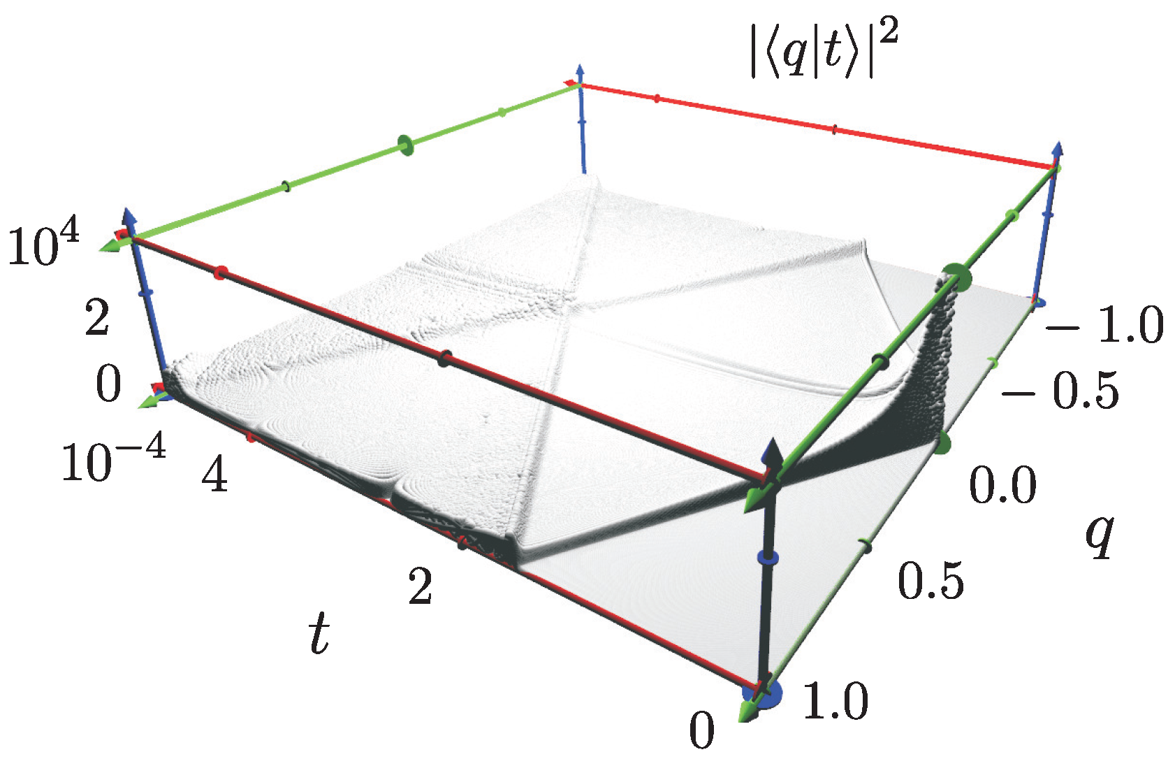
A three dimensional representation of the modulus squared of the time eigenstate ${\left|\langle q|t\rangle \right|}^2$, formed with the odd eigenfunctions $u_n^{(-)}\left(q\right)$ and coefficients $a_n\left(t\right)=e^{-it{E}_n^{(-)}/\hslash }$, can be seen in Figure 1. We see from the plot that the density follows the classical trajectories including the bouncing of the particle from the walls of the potential well.

Coordinate, momentum, and translations operations on equally spaced mesh points were studied earlier by other authors. [1,2] By considering equally spaced points on a finite interval, it was easy to introduce translations by discrete jumps and the periodicity of the mesh, extending, that way, a finite interval to an unbounded interval. However, not always do we find a set of points that are equally spaced, for example, the energy spectrum of some Hamiltonian operator $\widehat{H}$. Only in few cases there is an equal separation between the values of the energy spectrum. Non-equally spaced partitions of an interval allowed us to think on the possibility of performing more general than periodic translations, as was illustrated in this paper.

8. Conclusions

In conclusion, we can improve finite differences to the point of being exact, as it was shown in the example of the time eigenstate for the particle in an infinite well. There are many operators and functions that are in use in Quantum Mechanics theory. Thus we can find the exact finite differences for them.

We hope that our results will lead to a sound definition of a discrete momentum operator and to the discovery of a time operator in Quantum Mechanics.

References

- Santhanam, T.S.; Tekumalla, A.R. Quantum mechanics in finite dimensions. Found. Phys. 1976, 6, 583–587. [Google Scholar] [CrossRef]
- De la Torre, A.C.; Goyeneche, D. Quantum mechanics in finite-dimensional Hilbert space. Am. J. Phys. 2003, 71, 49–54. [Google Scholar] [CrossRef]
- Galapon, E.A. Self-adjoint time operator is the rule for discrete semi-bounded Hamiltonians. Proc. R. Soc. Lond. A 2002, 458, 2671–2689. [Google Scholar] [CrossRef]
- Asao, A.; Yasumichi, M. Time operators of a Hamiltonian with purely discrete spectrum. Rev. Math. Phys. 2008, 20, 951–978. [Google Scholar] [CrossRef]
- Asao, A. Necessary and sufficient conditions for a hamiltonian with discrete eigenvalues to have time operators. Lett. Math. Phys. 2009, 87, 67–80. [Google Scholar] [CrossRef]
- Torres-Vega, G. Universal raising and lowering operators for a discrete energy spectrum. Found. Phys. 2016, 46, 689–701. [Google Scholar] [CrossRef]
- Martínez-Pérez, A.; Torres-Vega, G. Exact finite differences. The derivative on equally spaced mesh points. submitted.
- Pauli, W. Handbuch der Physik Vol. 23; Springer: Berlin, Germany, 1926; ISBN 3-540-02289-9. [Google Scholar]
- Pauli, W. General Principles of Quantum Mechanics; Springer: Berlin, Germany, 1980; ISBN 3-540-09842-9. [Google Scholar]
- Martínez-Pérez, A.; Torres-Vega, G. Translations in quantum mechanics revisited. The point spectrum case. Can. J. Phys. 2016, 94, 1365–1368. [Google Scholar] [CrossRef]
- Gitman, D.M.; Tyutin, I.V.; Voronov, B.L. Self-Adjoint Extensions in Quantum Mechanics. General Theory and Applications to Schrödinger and Dirac Equations with Singular Potentials; Birkhäuser: New York, NY, USA, 2012; ISBN 978-0-8176-4400-0. [Google Scholar]
- Schmüdgen, K. Unbounded Self-Adjoint Operators on Hilbert Space; Springer: Heidelberg, Germany, 2012; ISBN 978-94-007-4752-4. [Google Scholar]
Figure 1.
Three dimensional plot of the squared modulus of the un-normalized time eigenstate, in coordinate representation , using 2000 energy terms. Dimensionless units. The probability has larger values around classical trajectories starting at , including the ones with zero, negative and positive momentum. We also can notice the bouncing of the particle from the walls.
© 2017 by the authors. Licensee MDPI, Basel, Switzerland. This article is an open access article distributed under the terms and conditions of the Creative Commons Attribution (CC BY) license (http://creativecommons.org/licenses/by/4.0/).
Share and Cite
MDPI and ACS Style
Martínez-Pérez, A.; Torres-Vega, G. Exact Finite Differences. The Derivative on Non Uniformly Spaced Partitions. Symmetry 2017, 9, 217. https://doi.org/10.3390/sym9100217
AMA Style
Martínez-Pérez A, Torres-Vega G. Exact Finite Differences. The Derivative on Non Uniformly Spaced Partitions. Symmetry. 2017; 9(10):217. https://doi.org/10.3390/sym9100217
Chicago/Turabian StyleMartínez-Pérez, Armando, and Gabino Torres-Vega. 2017. "Exact Finite Differences. The Derivative on Non Uniformly Spaced Partitions" Symmetry 9, no. 10: 217. https://doi.org/10.3390/sym9100217
Note that from the first issue of 2016, this journal uses article numbers instead of page numbers. See further details here.