On Elastic Symmetry Identification for Polycrystalline Materials


Department of Mathematical Modelling of Systems and Processes, Perm National Research Polytechnic University, Perm 614990, Russia
*
Author to whom correspondence should be addressed.
Symmetry 2017, 9(10), 240; https://doi.org/10.3390/sym9100240
Submission received: 17 September 2017
/
Revised: 14 October 2017
/
Accepted: 15 October 2017
/
Published: 20 October 2017
Abstract
:The products made by the forming of polycrystalline metals and alloys, which are in high demand in modern industries, have pronounced inhomogeneous distribution of grain orientations. The presence of specific orientation modes in such materials, i.e., crystallographic texture, is responsible for anisotropy of their physical and mechanical properties, e.g., elasticity. A type of anisotropy is usually unknown a priori, and possible ways of its determination is of considerable interest both from theoretical and practical viewpoints. In this work, emphasis is placed on the identification of elasticity classes of polycrystalline materials. By the newly introduced concept of “elasticity class” the union of congruent tensor subspaces of a special form is understood. In particular, it makes it possible to consider the so-called symmetry classification, which is widely spread in solid mechanics. The problem of identification of linear elasticity class for anisotropic material with elastic moduli given in an arbitrary orthonormal basis is formulated. To solve this problem, a general procedure based on constructing the hierarchy of approximations of elasticity tensor in different classes is formulated. This approach is then applied to analyze changes in the elastic symmetry of a representative volume element of polycrystalline copper during numerical experiments on severe plastic deformation. The microstructure evolution is described using a two-level crystal elasto-visco-plasticity model. The well-defined structures, which are indicative of the existence of essentially inhomogeneous distribution of crystallite orientations, were obtained in each experiment. However, the texture obtained in the quasi-axial upsetting experiment demonstrates the absence of significant macroscopic elastic anisotropy. Using the identification framework, it has been shown that the elasticity tensor corresponding to the resultant microstructure proves to be almost isotropic.
1. Introduction
The most important and promising trends in the development of modern material science are related to designing functionally graded materials for production of elements and structures with improved operating characteristics. It is well known that physical and mechanical properties of materials depend on their microstructures. Therefore, the control of their formation during different technological processes makes it possible to obtain desired macroscopic properties. Such problems are usually solved in two stages: first, an optimal microstructure is determined to fit each specific case, and then the process regimes are devised to create conditions for its formation. With this approach, the identification of parameters, which will provide the most adequate description of the developed material microstructure, is the matter of particular importance.
Numerous theoretical and experimental studies show that macroscopic properties of polycrystals significantly depend both on the physico-mechanical characteristics of the crystallites, and on their dimensions, forms and orientations. An essential change in the topological and stereological parameters of microstructure can be achieved with the use of thermomechanical treatment methods, which are related to severe plastic deformation. Control of the fragmentation mechanisms and rotational modes of inelastic deformation offers considerable scope for producing metals and alloys with a grain structure exhibiting the best properties for the preset operating conditions.
Different issues related to the problems of designing functionally graded materials are discussed, e.g., in [1,2,3,4,5,6,7,8,9,10,11,12,13,14]. General methodology of designing such materials based on multi-level modeling [15,16,17,18,19] is described in detail in [8].
In [2], the problem of minimization of the length of a flexible beam at a given deflection of its end is considered. The structure is supposed to operate in the elastic range under the constraint of the minimal value of the restoring force. An approach used by the authors involves an expansion of microstructure parameters including a crystallite orientation distribution function (ODF) into a Fourier series with respect to the generalized spherical harmonics [20]. The formulation of the optimization problem is developed in terms of the Fourier series coefficients. In [21,22], the same technique is used to maximize the load-carrying capacity of a plate with a circular hole, which does not produce inelastic deformation. Here, an optimal distribution of crystallite orientation is determined within the class of orthorhombic crystallographic textures. Estimates of the effective elastic moduli and yield strength for a polycrystalline aggregate with such symmetry properties are presented in [10].
An alternative way to represent ODF in a reduced form is considered in [1,4,5,11,12,13,14,23]. To control the texture-dependent parameters, a finite element representation of the ODF conservation equation [3,24] within a fundamental region of the Rodrigues space [24,25,26] is used. The inelastic strain evolution until desired properties are formed is determined by the gradient descent method. To accelerate the optimization procedure, the authors propose an approach that is based on the data-mining techniques applied to a specially organized database of microstructures [11,12,14,23].
Optimization of technological processing of the aluminum alloy sheet, using a direct multi-scale modeling method is described in [7,9]. In these studies, the numerical simulation is based on the finite element discretization of a computational domain on the macro- and meso-levels. Texture control is realized by correlating the grain orientation to the integration points of the mesoscopic representative volume element (RVE).
A characteristic feature of polycrystalline products obtained by plastic forming is a rather high inhomogeneity of the orientation distribution. By virtue of the fact that physical and mechanical characteristics of crystallites are anisotropic, such inhomogeneity provides, as well, anisotropy on the macro-level. Furthermore, the isotropy group [27] of such materials is usually not known a priori. The identification of the group elements, or in a more broad sense, determination of conformity of physico-mechanical properties with the known forms of anisotropy plays an important role in material design, thermomechanical treatment, strength analysis and subsequent exploitation of produced structural components and constructions. Knowledge of anisotropy type of a particular material allows one to simplify its constitutive equations, which are used for numerical implementation of the models describing different technological processes, and also to reduce the number of macro-experiments, which should be performed to identify its parameters. Moreover, there is a special interest in studying the relations between the microstructure and symmetry properties of the macroscopic RVE.
In this work, the emphasis is placed on the identification of the elasticity class, to which a Hookean solid belongs. One should note that the majority of papers on this topic focuses on the so-called symmetry identification problem, which is related to a search for orthogonal transformations, to which the elasticity tensor of the material under investigation is invariant.
A criterion of the existence of a symmetry plane for the elasticity tensor was obtained in [28]. The authors provide a theorem, according to which a material can be assigned to one of the six classes, depending on the number of such planes and their mutual orientations.
Another possible way to solve the identification problem is to examine a full system of algebraic invariants [29] of the elasticity tensors, which uniquely determine the material properties [30,31]. Such type of system, which has clear mechanical meaning but is not polynomial [32], is proposed in [31]. As mentioned in [31,33], for physical and mechanical problems the requirement that the invariants must be polynomial is not essential.
One can distinguish a group of techniques, which are based on the separation of an additive part of the elasticity tensor (e.g., by way projecting), possessing one or another type of symmetry [34,35,36,37]. In this case, the identification problem is reduced to determination of the symmetric part, which is the closest in some metric to a given tensor, as e.g., in [38,39,40,41,42,43,44,45]. Note that depending on the choice of the metric, the separated parts may have special properties.
It should be emphasized that the application of the above identification procedures implies knowledge of all elastic components of the examined material within some basis. Such information may be obtained, e.g., from the experiments [46,47,48] or by means of physically justified multi-level modeling. An approach that does not require preliminary determination of elastic constants is considered in [49,50,51,52,53]. In the cited works, a series of mechanical macro-experiments is proposed to identify the type of anisotropy of a Hookean solid.
The purpose of this study is to investigate changes in the elastic symmetry of polycrystals during inelastic deformation. To this end, the results of the numerical experiments obtained in the framework of the multi-level crystal elasto-visco-plasticity model described in [54] for a polycrystalline copper RVE are analyzed. The experimental program includes simple shear, quasi-axial tension and upsetting tests. To solve the symmetry identification problem, a “projection” approach [44] is used.
This paper is organized as follows. In Section 2, the notation and definitions used in the paper are refined. Section 3 is devoted to formal classification of elastic materials and general approach to identification of classes, which is based on a special approximation of the elasticity tensors. In Section 4, the application of the proposed identification procedure for investigation of elastic properties of polycrystalline RVEs is considered. In Section 5, the results of the analysis of changes in elastic symmetry of polycrystalline copper revealed by the numerical experiments on inelastic deformation are presented. The paper ends with a discussion, where particular attention is paid to some problems related to determination of crystallographic textures characterized by a desired macroscopic symmetry of elastic properties, and a conclusion.
2. Preliminaries
In what follows, the notations and definitions formulated in this section will be used.
Let be a three-dimensional Euclidean space over the real field, (it is specified as in the case of the complex field, ); () is the space of the -rank tensors over (); () is the orthogonal (proper orthogonal) group of transformations of . signifies the tensor of rotation about the axis by the angle . Let be an arbitrary vector basis and be its conjugate, such that , where is the Kronecker symbol.
For brevity, the tensor product of and is written below as , i.e., by omitting a sign of the operation.
Let the dot product, «», of and be defined by the formula (hereinafter the summation convention for repeated indexes, which are not in parentheses, is adopted):
The following definition for the double dot product, «», of and is being used:
With respect to this product, is a unital non-commutative algebra [55] with the second isotropic tensor, [56], taken as the unit element, i.e., holds for any . In such algebra, the Eigen-value problem for is stated as follows.
Find the values of such, that the equation (either of the two equations):
with respect to has non-trivial solutions.
In the following, and defined by (3) are termed the Eigen-values and the right (left) Eigen-elements of , respectively. In total, such tensor has nine Eigen-values (multiple values are counted).
By definition [57], has the major symmetry if the requirement, , is satisfied for any basis. Similarly, the minor symmetries take place when the equalities, and , hold. Note that if a tensor possesses both the major and minor symmetries, it generally has 21 independent components.
It can be shown that all Eigen-values of a major-symmetric are real. Such tensor can be written as (spectral decomposition):
where and are the Eigen-values and normalized (i.e., ) Eigen-elements of , respectively. It should be emphasized that a tensor possessing both the major and minor-symmetries always has a zero Eigen-value of multiplicity 3, the Eigen-subspace of which involves all antisymmetric 2-rank tensors.
The above product has such a property that for all and . Let signify the symmetry group of .
Finally, the definition of the total scalar product, «», of and is given by the formula:
It should be remembered that this operation gives rise to the Frobenius norm [59], :
and allows the space, , to be treated as a Hilbert space. Moreover, for the further treatment it will be interesting to consider the so-called operator norm, , defined on the space :
where is the null tensor. This norm treats as a linear operator, , obeying the rule . Let the kernel and the image of such operator be denoted as and , respectively.
Given any , it is possible to decompose into the direct sum: , where is the subspace uniquely determined by . The operator, , governed by satisfies the conditions, and , and hence [60] is invertible. The tensor, , associated with the inverse operator, , (so that ) will be called the generalized inverse of . Such tensor has the property that holds for all . Also, if is of the form (4), then can be represented as follows:
In the case of a trivial kernel, the generalized reversibility of a tensor is equivalent to the algebraic one.
3. Elasticity Class Identification
Suppose that the examining material is simple and its elastic deformation is governed by the generalized Hooke’s law [61]:
where is the Cauchy’s stress tensor, is the small strain tensor, is the elasticity tensor. It should be noted that, in the general case, in the capacity of such equation, an arbitrary, physically linear constitutive equation could be used, including the one that relates the velocity measures of stresses and strains.
For a Green elastic material [62], the existence of a potential implies that its elasticity tensor has a major symmetry. Recall that in the framework of the classical elasticity theory, which operates with the symmetric measures of stresses and strains, there should also be minor symmetries, so that in the general case has 21 independent components.
It seems reasonable to describe the classification of materials based on their elasticity tensors in greater detail. First, define the congruence relation, «», between two linear subspaces, , in such a way that holds if and only if there exists a tensor such that . As it is readily seen, this is an equivalence relation, so that it can be used to form the quotient set, , from the set, , of all subspaces of . The elements of are the classes of congruent subspaces. It seems reasonable to associate any with , if contains a subspace, to which belongs. In this regard, a union of all congruent subspaces contained in the element is considered to mean the class of 4-rank tensors, , or, in the related context, the elasticity class. Given some representative subspace, , the following definition can be written: . Thus, any class is uniquely specified by some subspace in . One should also note that although each of these subspaces belongs to exactly one element of , their tensors might belong to several classes simultaneously.
Let be a class of elastic tensors with as a representative subspace. Here and below, this upper symbolic index, , will be used to specify the considered class in the framework of the accepted classification. By definition, any has the following form:
where are arbitrary independent constants (), is some orthogonal tensor, and are the prescribed linearly independent tensors. It is readily seen that each class is uniquely given by its own set of the base tensors, . Suppose that these tensors are determined in terms of the orthogonal, normalized basis, , of the laboratory coordinate system (LCS). Then, as it follows from the structural Formula (11), in the basis, , , the multi-dimensional matrix of will have the known structure, which is characteristic of . Bearing this in mind, this basis will be termed canonical.
In continuum mechanics, the classification, which is based on the concept [27] of isotropy group with respect to an undistorted configuration, has received wide acceptance. As demonstrated, e.g., in [63,64], the elasticity tensor can be assigned to one of the eight symmetry classes according to its invariance with respect to transformations of the orthogonal coordinate system. These classes consist of tensors with congruent (orthogonally conjugate) symmetry groups. The structure of such class allows its representation as the union, , where is the subspace of tensors invariant with respect to a given subgroup of orthogonal transformations(which, accurate to an orthogonal transformation, is the symmetry group of tensors from this class). Depending on cardinality of these groups and directions of the inclusion between them, the symmetry classes can be hierarchically schematized as shown in Figure 1.
In this paper, particular attention is paid to the cases of isotropy, transverse isotropy, cubic symmetry and orthotropy. The structure of tensors, which can be taken as the basis ones for the above-mentioned classes of symmetry, is shown in Table 1 (indexes of non-zero components and their corresponding values in the canonical basis are given). The parameters, , of decomposition (11) with respect to these tensors are, in essence, the non-zero independent components of in the so-called principal axes of anisotropy [53], i.e., in the basis, for which the number of such components is minimal. Note that for isotropic and transversely isotropic classes the systems of the tensors given in the table are not biorthogonal.
Generally speaking, the classification structural Formula (11) can be constructed based on the arbitrary additive decomposition of an elasticity tensor, which, in the general case, bears no relation to the elasticity symmetry groups. In particular, it is possible to use the spectral decomposition (4) (the major symmetry of is taken into account):
where and are the Eigen-values and the corresponding normalized (i.e., ) Eigen-elements of , respectively. It is evident that by grouping the Eigen-projectors, , associated with multiple Eigen-values, , Formula (12) can be reduced to (11). It should also be noted that the base tensors obtained with such approach turns to be “”-biorthogonal. Similar elasticity tensor decompositions were used, e.g., in [30,65,66,67].
Let the elasticity class identification problem (ECIP) be formulated as follows.
All components of an elasticity tensor are given in the LCS. It is required to determine, which of the classes under consideration this tensor can be assigned to with a desired accuracy.
Good reason for assigning the examined material to a given elasticity class, , is the existence of class approximation, , for its elasticity tensor, , such that the norm of the residual of a stress tensor (or the analogous stress measure) in relation (10), , is quite small on the bounded subset of . Adopt the notation: . A quantity , where is a mapping, such that the inequality
holds for each , will be called the mismatch estimate (ME) for with respect to . Thus, the problem of assignability of to a given can be reduced to a minimization of over an admissible set of tensors from .
In its turn, the function, , introduces a “closeness measure” for the tensor-argument, which determines how close it matches the class . Note that, if mapping is continuous for all , then the above function is also continuous. For completeness of presentation, this statement is proved below by formulating its sufficiently general case as a lemma. Let be a metric space with a distance function, ; and are the nonempty sets; is a given functional. The following proposition is true.
Lemma 1.
If is continuous at for all , then the functional, , defined by is also continuous at .
Proof.
Under the assumption of the lemma, for any and there exists such that, for all , satisfying the condition , the following relation holds true:
Then, according to the definition of infimum in the real numbers, there are such that and . From the same definition it follows that and . Thus, for these elements, it is possible to write:
Hence, can take an arbitrary small value if an appropriate value of is chosen. This means that is continuous at . □
The lemma is proven.
A tensor meeting the condition will be called the optimal approximation of in . If necessary, a method for constructing the objective function, , will be specified. Given a ME for the optimal approximation of an elasticity tensor, one can say about compatibility (incompatibility) of this tensor with the related class.
A sufficiently reasonable constraint on is the fulfillment of when and only when . In particular, this condition permits the use of a metric or a norm defined on as such mapping. In general, if the above requirement is met and the function is continuous everywhere, then will be called the mapping, which defines a natural ME.
Note that holds for all . However, in the case when the elements fall within the Eigen-subspace of , which has the maximal in modulus Eigen-value, the above relation degenerates into an equality. In this sense, the operator norm (8) gives an exact upper bound for a residual of the class approximation, which justifies treating as an objective function in estimating the class compatibility of . However, it would seem that the formulation of the corresponding optimization problem in terms of the Frobenius norm (7), which implies minimization of the alternative quantity, , is computationally more efficient. This norm specifies an upper bound (and hence, a rougher ME) of the operator norm, i.e., . Then, an equality of the above written quantities takes place if and only if has one (with regard to multiplicity) non-zero Eigen-value. One should note that the existence of the major and minor symmetries provides the following lower bound: , which degenerates into an equality, when and only when has the only hextuple non-zero Eigen-value.
The value of ME is associated with the maximal absolute error, which occurs in stresses determined by the generalized Hooke’s law when approximating the elasticity tensor. To characterize a relative error, one can define , where is the generalized inverse of . This quantity will be called the relative mismatch estimate (RME) for with respect to . It can be easily verified that the RME satisfies the following inequality for each :
In the present work, the optimization problems are formulated essentially with the use of the Frobenius norm. Some specific features related to the statement and solution of such problems should be discussed.
Due to the fact that all subspaces in are the Hilbert ones, the -optimal approximation, , by its structure, is an “”-orthogonal projection of onto . Such projection satisfies the condition: . Hence, minimization of the quantity is tantamount to maximization of . Moreover, the Frobenius norm properties imply that . Thus, an optimization problem for evaluating an -optimal approximation can be stated as the problem of maximization only with respect to :
Problem 1.
Find such that:
Or, in the case where is a “”-biorthogonal base system:
Problem 2.
Find such that:
As shown in [35], projecting a tensor onto a subspace, which is invariant to some orthogonal subgroup, is equivalent to averaging [68] this tensor over the same subgroup. Thus, adhering to the symmetry classification of elasticity tensors, one can write:
Here is the symmetry group of tensors from and , where is the Borel sigma-algebra on , is the normalized (i.e., ) Haar measure. In such a case, an optimization problem equivalent to Problem 1 (2) can be stated as follows:
Problem 3.
Find such that:
For a finite symmetry group, an integral in Problem 3 is an arithmetic mean of the integrand values on the elements of this group. Due to this fact, averaging in (23) may have computational advantage over projecting in (18)–(19) or (20) (8)–(10) when searching for -optimal approximations in the symmetry classes, the groups of which have relatively few elements.
One should note that in the case of transverse isotropy the number of elements required for averaging might be reduced to a finite set. Such a feature directly follows from Hermann’s theorem [69], which asserts that the invariance of a to the transformation, , for a natural implies its invariance to the group of transformations, . Indeed, adhering to the line of reasoning presented in [35], it is possible to easily demonstrate that at a given natural number, , and any and , the quantity, , turns out to be an “”-orthogonal projection of onto the subspace in , which is invariant to the group, . Then, by applying Hermann’s theorem, one can conclude that this projection is also invariant to , i.e., is transversely isotropic along the vector . In particular, this result implies that five elements will suffice to average an elasticity tensor over the group of transverse isotropy.
Problem 1 (2, 3) always has a solution, but, in the general case, it is not unique. Indeed, as it can be readily shown, holds for all and . Hence, if is an -optimal approximation of from , then is also the approximation of such kind. This makes possible to reduce the admissible set of Problems 1–3 to the subset, , such that . Moreover, since the Rayleigh product of an even-rank tensor by yields the same result as the product by , it will suffice to consider only special orthogonal tensors from . Thus, when searching the -optimal isotropic approximation of , an optimization is not required at all. This approximation is uniquely determined so its expression can be written explicitly. It is consistent with the isotropic part of , the concept of which is introduced by Voight [70]. Furthermore, in the case of a -optimal transversely isotropic approximation, only the orientation of its isotropy axis can be used as an optimization parameter.
Non-negativity of the elastic potential imposes the condition of positive definiteness on (hereinafter in the sense that for all ). Such condition is desirable for approximating tensors as well. In [35], it is shown that positive definiteness of a 4-rank tensor holds during its averaging over the orthogonal subgroup. Due to equivalency of this operation to the “”-orthogonal projection, one can conclude that in the symmetry classes the -optimal approximations of a positive definite tensor are also positive definite.
The mentioned features of the Frobenius norm are quite strong arguments in the favor of using this norm in numerical calculations. Nevertheless, optimization problems analogous to Problems 1–3, can be formulated in terms of quite arbitrary metric on . Various ways to define such metric are considered, e.g., in [34,36,37,40]. In [36], the symmetric approximations of elasticity tensors are constructed with the use of different approaches, which are based on the Frobenius, Log-Euclidean and Riemannian distance functions. The last two, compared to the first one, possess some additional invariance properties: in particular, with regard to inversion of the tensor-arguments. In [34], the specific features of the operator norm, , are investigated theoretically, when searching for the -optimal elasticity tensor approximations. It was shown that the -optimal approximation of a positive definite tensor, unlike the -optimal one, may be not positive definite or unique in some degenerate cases. The results for the evaluation of the - and -optimal approximations in the transversely isotropic class and their comparative analysis are presented in [40].
Going back to the ECIP, suppose that is the -optimal approximation of , i.e., the solution of Problem 1 (2, 3) in . Adopt the notation: . Then the following chain of inequalities holds:
Since is the exact upper bound for the norm of the residuals of all possible approximations, both and give the MEs for , among which is more accurate. Its values (or the values of the associated RME, ) for different classes, which are arranged in the non-increasing order, form the hierarchy of class approximations, each of which can be accepted with one or another error level. The construction of such hierarchy is understood as a solution of the ECIP. In its turn, the implementation of this procedure implies the statement and solution of Problem 1 (2, 3) in all classes considered in the framework of the adopted classification. It is worthy to recall again that here does not generally minimize the norm and, hence, does not provide an exact upper bound for the residual norm of the class approximation. Nevertheless, it can estimate the latter as:
It should also be noted that, as in the case of the Frobenius norm, keeps its value in the family of tensors of the form , where and .
In the space of optimization parameters, the topology of the hypersurfaces defined by the objectives of Problems 1–3 is generally rather complex. There may exist multiple local and global minimums, so that the direct use of determined numerical methods is obstructed. However, for the majority of practical applications, there is no need for an exact approximation of the solutions to a global minimum, so that the optimization problems can be solved by using the heuristic algorithms, e.g., the particle swarm optimization method [71] employed in [39,41]. It seems plausible to use as a criterion of assigning a material by its properties to one or another class a small value of the residual caused by the related approximation in its constitutive equation. Hence, the possibility of obtaining an acceptable upper estimate for this value gives a convincing reason for such assignment.
In what follows, three types of the quantities, which characterize MEs for the class approximations obtained by the numerical global optimization, will be considered. Each of them is shortly defined in Table 2. All positive definite tensors from a specified class are taken as an admissible set for approximations being optimized. Also, three types of RMEs will be used. They are supposed to be introduced by multiplying the associated MEs just as before, by the maximal Eigen-value of the generalized inverse of an elasticity tensor under approximation.
4. Elasticity of Polycrystalline Aggregates
During the multi-level modeling of a material, its macroscopic physical and mechanical characteristics are being obtained by averaging the similar properties of its structural elements on the subjacent scale levels. For a single-phase polycrystal, the RVE of which consists of crystallites with the same specific weight, the simplest variant of the averaging operation can be written as:
Here is the number of crystallites in the material’s RVE, is the macroscopic elasticity tensor, is the elasticity tensor of a single crystallite and are crystallite orientation tensors. Further study is restricted to using only this form of averaging, which is also known as averaging by Voigt. Such definition refers to that the effective elasticity tensor obtained from (26) establishes a relation between the stress tensor averaged over crystallites and the macroscopic strain tensor under the assumption of the Voigt hypothesis. It should be remembered that there exist more complex and physically justified homogenization procedures, which consider additional stereological parameters of the internal structure [72].
Given a statistically uniform distribution of crystallite orientations in a polycrystal, its physical and mechanical properties are assumed to be isotropic. However, due to the presence of stochasticity, one can speak only approximately about compatibility of the properties under consideration with any of the classes. Numerical estimation of this proximity degree makes possible to determine the size of the RVE of the polycrystal being investigated, which is essential in the context of constructing the multi-level models and determining its parameters.
Consider a polycrystalline aggregate of crystallites with random orientations, . Suppose that defines a natural ME. Then, is a real-valued random variable (in the sense that for any subset from the Borel sigma-algebra on its pre-image belongs to the Borel sigma-algebra on ). The concept of convergence of the aggregate elasticity tensor to a class, as the number of crystallites increases, can be formalized as follows. The elasticity tensor, , of a polycrystalline aggregate of crystallites converges to a class, , as if
Note that from (26) it follows that , so that at a fixed a random sequence, , is uniformly bounded. Thus, with respect to continuity, is also uniformly bounded. Condition (27) implies that this sequence converges almost surely. Hence [73], it will also converge in the mean, i.e.,:
where is the mathematical expectation.
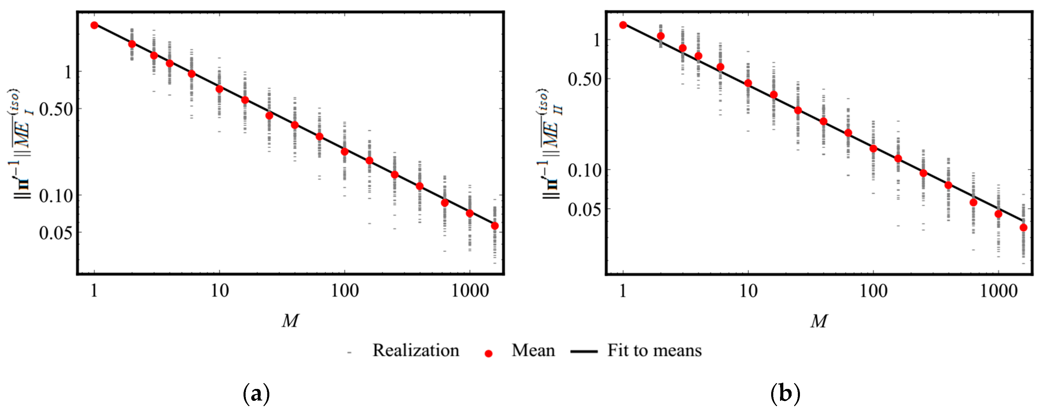
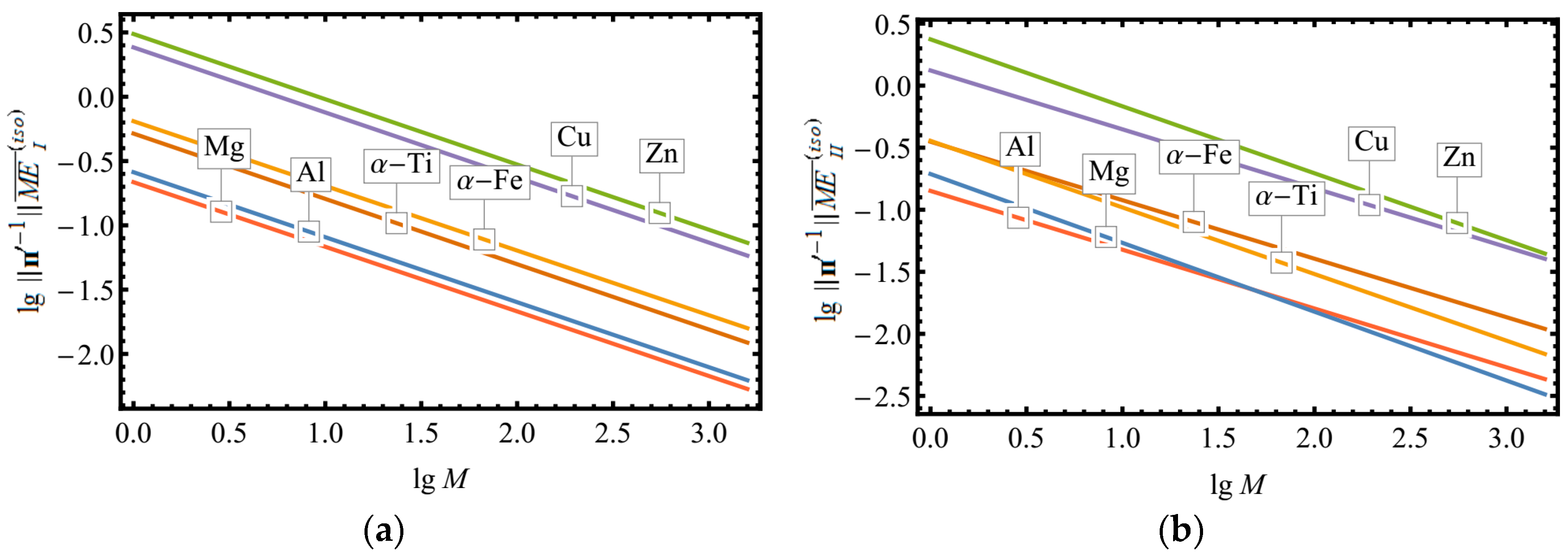
Given a uniform orientation distribution, due to (28) an empirical estimate of or can be used to evaluate the level of accuracy, to which an aggregate of crystallites can be considered as an RVE of the simulated polycrystal. In Figure 2, such estimates are constructed for polycrystalline copper. For each fixed number of crystallites, , an independent repeated sampling of 100 realizations of polycrystalline aggregates with uniformly distributed random orientations is generated. Then, the values of and corresponding to the obtained realizations are calculated and their sample means, and , are evaluated. The dependences of these mean values on are approximated by the power functions as and . Here, are the parameters determined by the logarithmic least-square method. The values of these parameters for aggregates of some metals are given in Table 3. Regression curves (straight lines on the log-log plot) are presented in Figure 3. The obtained results make possible to estimate the necessary number of crystallites in a macroscopic polycrystalline sample, which is statistically representative for a given margin of error. In [74,75], similar estimates are constructed for relative standard deviation of macroscopic Young and shear moduli, which are obtained for single- and double-phase polycrystals by Hill’s averaging [76].
5. Changes in Elastic Symmetry of Polycrystals during Inelastic Deformation
In polycrystals, severe inelastic deformation is usually accompanied by a significant reorientation of their anisotropic crystallites, in which the symmetry of physical and mechanical characteristics is determined mainly by their lattice type. The symmetry of analogical macroscopic properties depends on polycrystalline texture and is able to change during such processes.
In this section, the results of the numerical investigation of changes in the elastic symmetry of the RVE of a single-phased polycrystalline copper during inelastic deformation are presented. Simple shear, quasi-axial tension and upsetting tests are considered. The crystallite orientation distributions are obtained with the help of the two-level crystal elasto-visco-plasticity model discussed in [54]. The equations for the co-rotational spins, , of the crystallites are taken from [77]:
Here, are the velocity gradient tensors of elastic deformations and the bases, , are introduced in such a way that, at each moment, are the normalized crystallographic vectors, are the unit vectors from crystallographic planes, which satisfy , and . For each crystallite, its elasticity tensor is assumed to be constant with respect to the associated system of the defined vectors.
The applied mechanical loads are kinematical and their deformation gradient tensors are of the form: , where is a velocity parameter (which takes a constant value in the examined processes), is the current time and is the duration of the process considered. The magnitude of deformation accumulated in the material to time is characterized by the parameter, . MEs are evaluated for isotropic, transversely isotropic, cubic and orthotropic classes (the short symbolic indexes are iso, tra, cub and ort, respectively).
The sequence of computational operations is as follows. First, a polycrystalline aggregate of crystallites with a random uniform orientation distribution is generated. At each moment of the simulated deformation process, the components of the macroscopic elasticity tensor are calculated by applying the averaging procedure given by (26). For the examined classes, the parameters of the -optimal (and, in the case of isotropic class, the -optimal) approximations of this tensor are obtained by solving numerically Problem 1 (2, 3). The next step is to calculate the RMEs (corresponding to the above mentioned approximations), which are taken to be the values of and (), forming a hierarchy of elastic symmetry classes at the current deformation stage.
For the obtained cubic and orthotropic approximations, the orientations of their canonical bases are presented with the help of the Euler angles: , and . These parameters describe the rotational transform, , in (11) as follows:
In the further figures, their values are provided for all tensors of the form , , where is a numerical solution of Problem 1 (2, 3), and the groups, , consist of the following elements:
In the case of the orthotropic approximations, the base tensors are ordered so that their sequent longitudinal elastic moduli decrease.
To characterize the transversely isotropic approximations, the spherical orientation angles of their isotropy axes are considered: and . Using these parameters, the mentioned approximations can be evaluated by substituting into (11) where is the unit vector directed along the isotropy axis. In such a case, the following parametrization takes a place:
In the related figures, the orientation angles are plotted for the obtained direction vectors, , together with the angles for .
In the initial configuration (), the elasticity tensor of the examined polycrystalline realization has the following component matrix (in the LCS basis; the Voight notation is used):
With an acceptable accuracy, this tensor can be treated as an isotropic one; the value of corresponding to it does not exceed 1.89%.
5.1. Simple Shear
The deformation gradient tensor of the realized loading regime is , where . The numerical calculation is carried out until . The direct pole figures (DPFs) for the basic crystallographic directions corresponding to different deformation stages are depicted in Figure 4.
Noticeable inhomogeneity of the orientation distribution acquired by the aggregate causes weakening of isotropy of its macroscopic elastic properties, as evidenced by the growth of the corresponding RMEs shown in Figure 5a. It is worthy of note that in this process the values of and almost coincide. An analogous growth of RMEs also holds for other symmetry classes as demonstrated by changes in and shown in Figure 5b and Figure 6. At the sufficiently high levels of accumulated deformations, the error in the assignment of the material to the elastic orthotropic class significantly increases, so that more suitable approximations can be searched for within the monoclinic class. The families of the orientation parameters for the calculated approximations are presented in Figure 6.
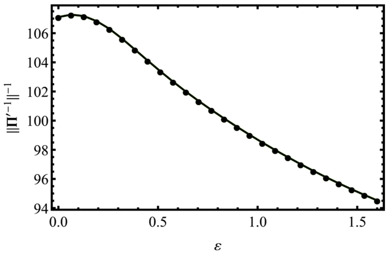
The dependence of (which is equal to the minimal non-zero Eigen-value of ) on the loading parameter is shown in Figure 7. This quantity is a multiplier which turns an RME to the associated ME. Due to a relatively small range of its values, the results presented for RMEs turn out to be qualitatively similar to the results obtained for MEs.
5.2. Quasi-Axial Tension
The deformation gradient tensor of the realized loading regime is , where . The numerical calculation is carried out until . The DPFs for the basic crystallographic directions at different deformation stages are depicted in Figure 8.
The RME curves of the aggregate elasticity tensor for the isotropic class are given in Figure 9. As it is readily seen, the growth of the obtained estimates is monotonic, therefore in this case also, inhomogeneity of the orientation distribution leads to weakening of the macroscopic elastic isotropy. One can point out that and are close to each other, especially at the initial deformation stages.
The variation of RMEs in other symmetry classes is presented in Figure 9b and Figure 10. Weak incompatibility with transversely isotropic and orthotropic classes holds at all stages of the process under examination. It means that the material retains the orthotropic and transversely isotropic properties. At the same time, the RMEs in the cubic symmetry class increase, which testifies to weakening of the related symmetry properties. The families of the orientation parameters for the calculated approximations are provided in Figure 10.
The results obtained for MEs are similar to the results presented for RMEs. The transition multiplier curve is plotted in Figure 11.
5.3. Quasi-Axial Upsetting
The deformation gradient tensor of the loading regime is given as , where . The numerical calculation is carried out until . The DPFs for the basic crystallographic directions at different deformation stages are depicted in Figure 12.
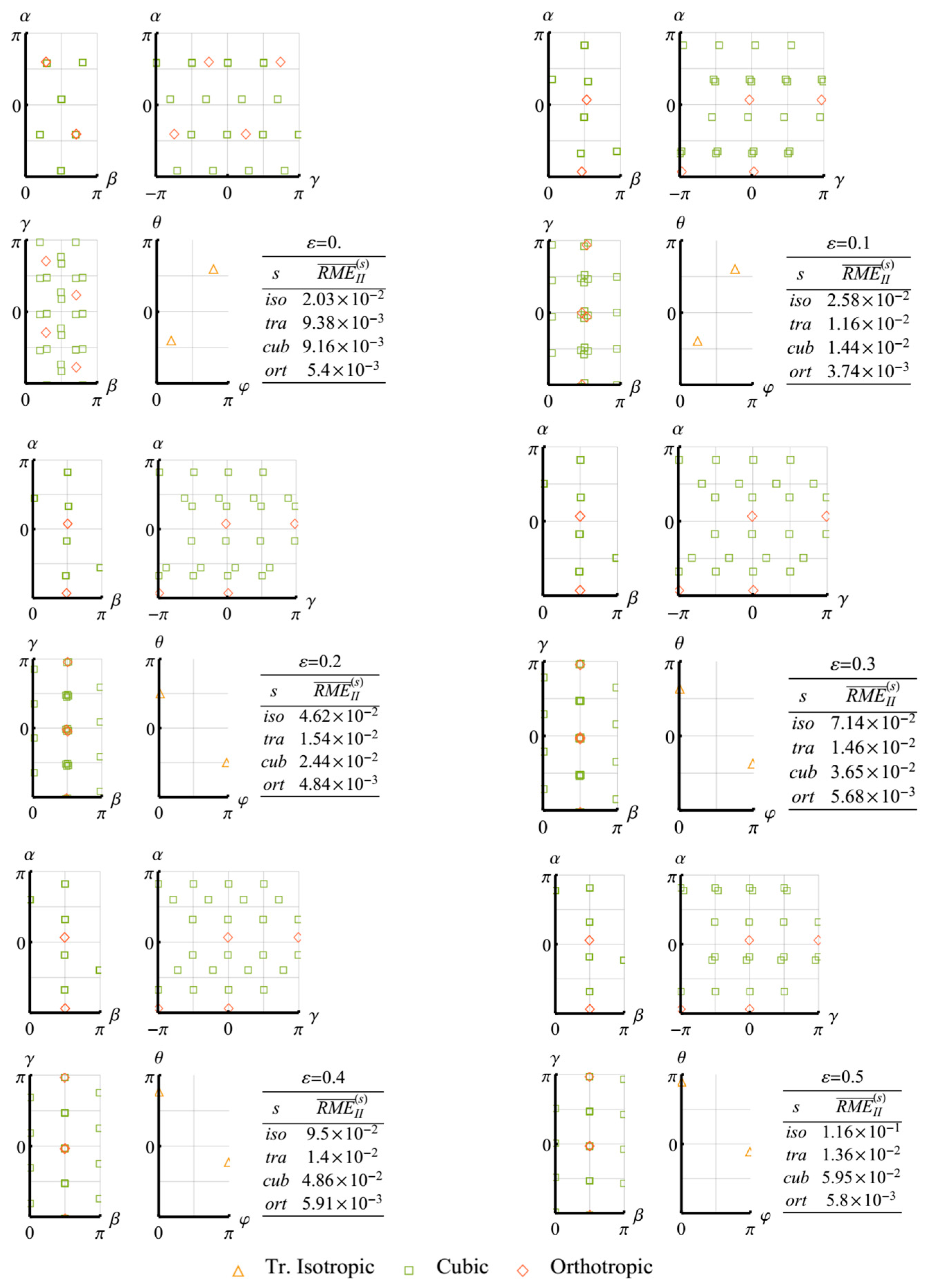
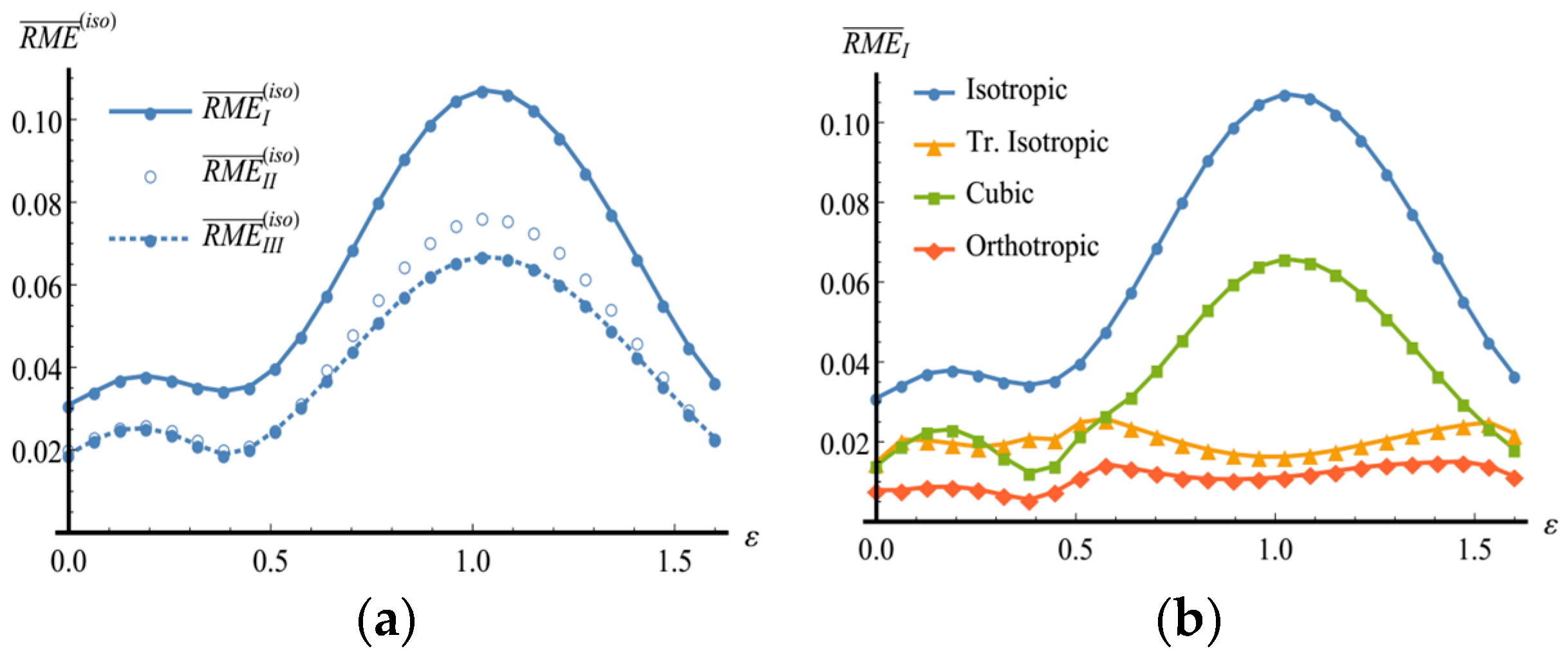
Changes in RMEs in isotropic class are presented in Figure 13. A characteristic feature of these graphs is their essential non-monotonic character. Within certain intervals of the deformation process, the aggregate elastic properties are found to be close to isotropic ones despite noticeable inhomogeneity of the orientation distribution observable on the DPFs Worthy of note is the fact that at the end of the examined process the RMEs in the isotropic class practically regain their initial values, while the aggregate attains a pronounced crystallographic texture. Such result speaks in favor of feasibility of textures with isotropic macroscopic elastic properties in polycrystalline materials. Note that in the case under consideration and also take close values.
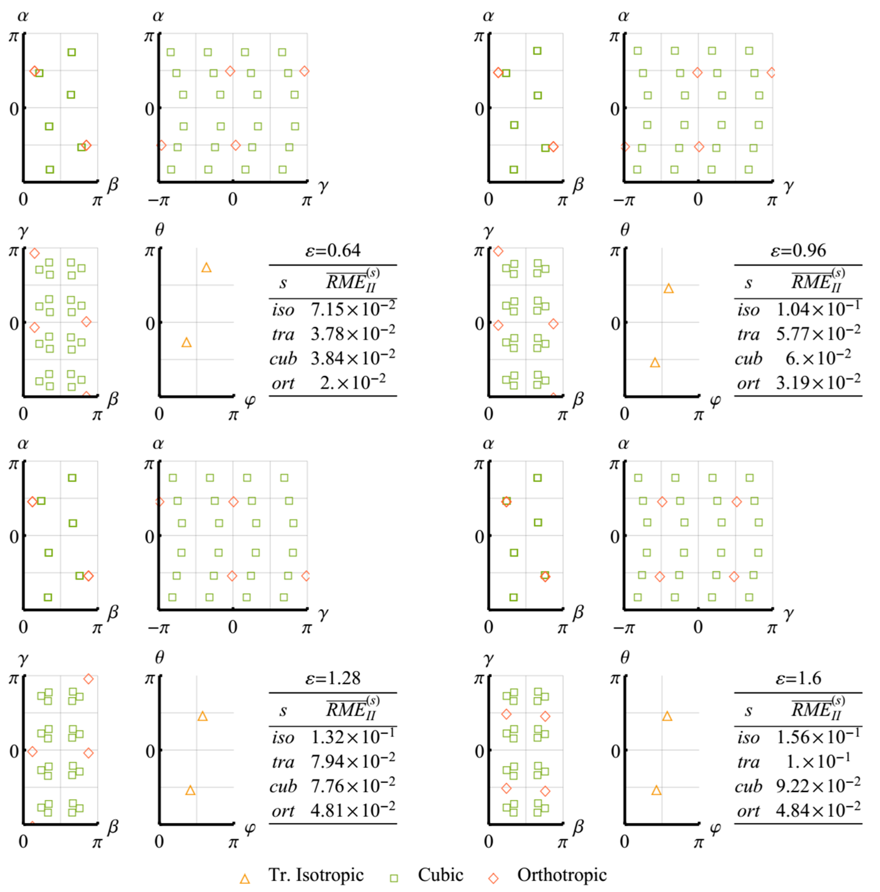
The dependences for RMEs in other symmetry classes are shown in Figure 13b and Figure 14. Incompatibility with the transversely isotropic and orthotropic classes changes insignificantly. In the cubic symmetry class, the observed dependence is analogous to that obtained in the case of isotropy. The incompatibility maximum occurs at . The families of the orientation parameters for the calculated approximations are given in Figure 14.
The graphs of the MEs variation are similar to those obtained for RMEs. It is to be noted that the transition multiplier changes non-monotonically, too. Its curve is plotted in Figure 15.
6. Discussion and Conclusions
The presented investigations have revealed a peculiar feature of the examined quasi-axial deformation processes, which is the retention of elastic orthotropy and transverse isotropy. Moreover, an additional examination has shown that at the loading stages characterized by quite strong incompatibility (increase of a RME by more than two times compared to its initial value) of the material with higher symmetry classes the deviation of the identified isotropy axis from the direction vector of the process, , proves to be small (does not exceed: for the tension and for the upsetting processes). A similar situation holds for deviation of one of the rotation axes to be determined in the orthotropic class (does not exceed: for the tension and for the upsetting processes). These results are consistent with the supposition of the relationship between the symmetry properties of a deformation process and the elastic properties of a material under deformation.
According to the results of the numerical investigation, the process of quasi-axial upsetting of a polycrystalline aggregate can involve the formation of inhomogeneous orientation distributions, for which the macroscopic elastic properties are close to the isotropic class. Theoretical substantiation for the existence of such textures can be obtained, e.g., by studying the problem of determining a discrete orientation set, , which minimizes for a given . It can be shown that this problem is equivalent to the following one.
Problem 4.
Find such that:
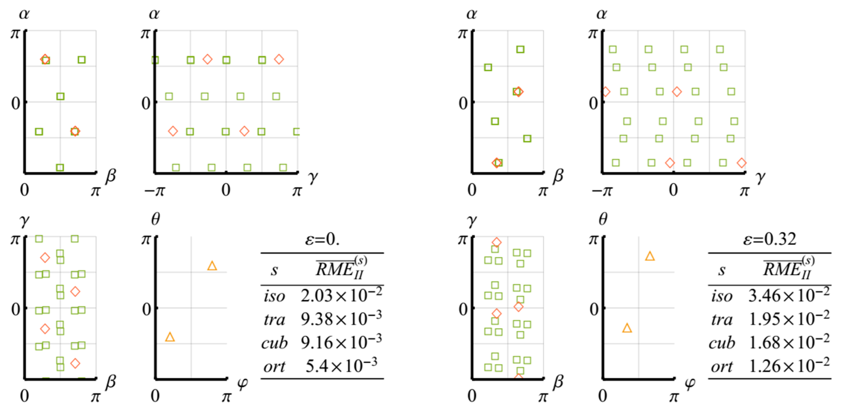
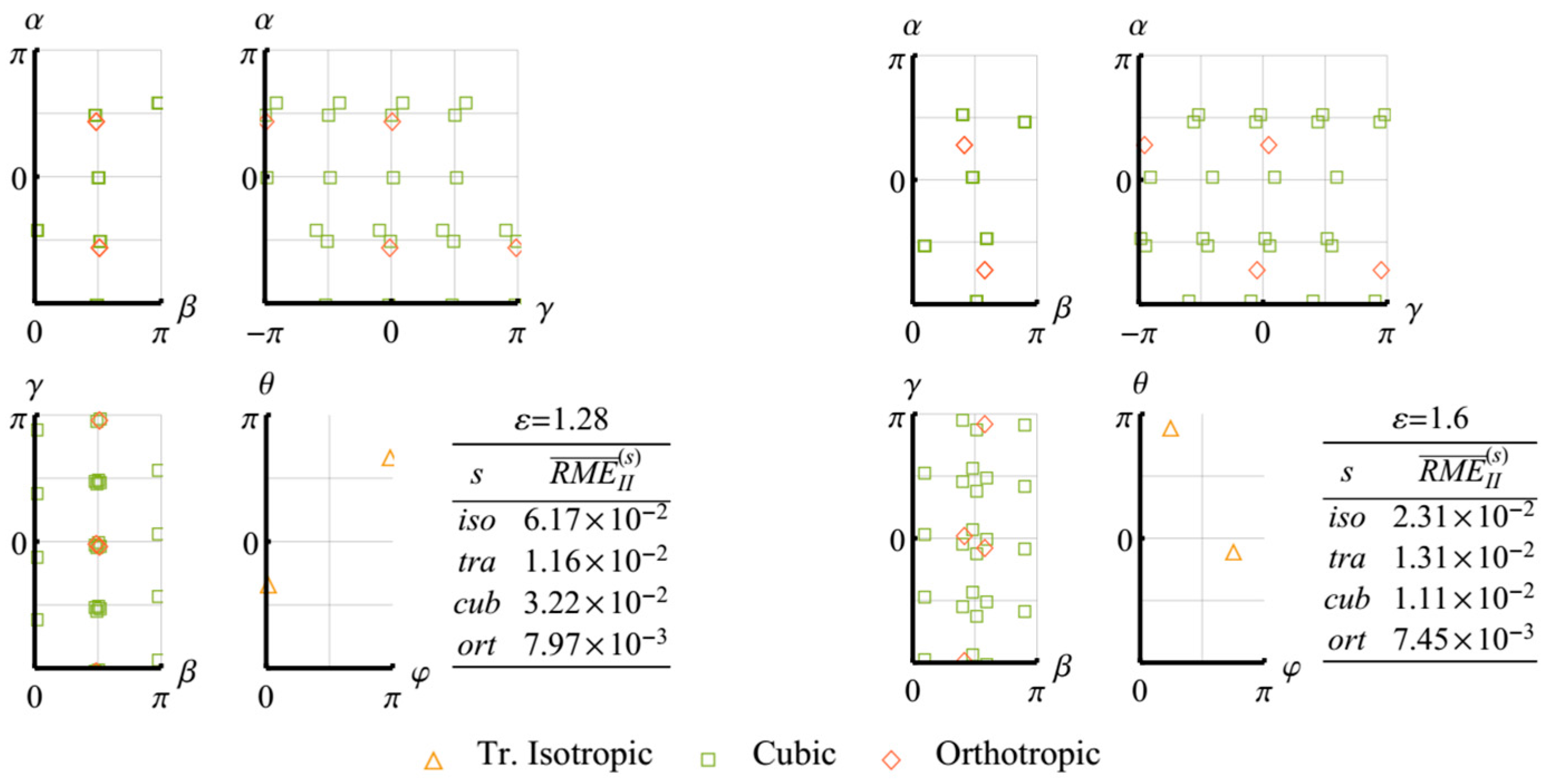
Here, can be associated with the number of orientation modes, over which the crystallite orientations are distributed in equal proportions. Problem 4 has at least a one-parametric family of solutions, which differs from one another by a Rayleigh product with an arbitrary orthogonal transformation. MEs for the -optimal isotropic approximations () and the associated RMEs () with respect to the elasticity tensors obtained for the polycrystalline copper aggregates with optimal orientation modes are summarized in Table 4 for . Such modes for are depicted on the DPFs for the basic crystallographic directions.
It should be pointed out that, as shown in [79], in the case of even , for crystallites with cubic elastic symmetry there always exists a set of orientations, over which averaging of the form (26) results in isotropy of macroscopic elastic properties. A configuration of such orientations for is described in [78]. It coincides with the configuration presented in Table 4.
Similar sufficient conditions for transverse isotropy can be obtained by virtue of Hermann’s theorem. It can be readily proven that if the rotation axis, , of the phase characteristic tensor, , is of order , then an effective characteristics tensor of the form , where , is transversely isotropic along for . In particular, this implies that, for transverse isotropy of elastic properties of a single-phase polycrystal consisting of cubic symmetric crystallites, two orientation modes will suffice. It can be also of interest to find textures, which show the best fit to a given macroscopic elasticity class, . In terms of the orientation measure [80], , where is the Borel sigma-algebra on , and the ME function, , such problem can be formulated as follows:
Problem 5.
Find such that:
where is the admissible set, is the space of probability measures defined on . One should remark that if satisfies the conditions of Lemma 1, then the functional of Problem 5 is bounded in .
In conclusion, it should be also mentioned that and , i.e., the operator norms of the - and -optimal isotropic approximations, respectively, obtained in the numerical experiments, are close to each other. Since from the computational viewpoint the advantage of the Frobenius norm is quite evident, the choice of this norm for solving the ECIP seems quite reasonable.
To sum up, in the presented work, the problem of determining the elastic anisotropy type of polycrystalline materials is discussed. The concept of 4-rank tensor class as the union of congruent specially structured subspaces was introduced. This definition makes it possible to formally classify the elasticity tensors allowing the classification by their symmetry properties. The problem of identification of the linear elasticity class for a material with elastic moduli known in some basis was formulated. To solve this problem, a general approach based on the approximation of the elasticity tensor by the class analogies was proposed. Residual estimates of such approximations governed by a linear elasticity law form a hierarchy of classes, to which the examined material can be assigned according to their elastic properties with sufficient accuracy. The formulated mathematical framework was then applied to theoretical study of single-phase polycrystalline elasticity. For some metals, the dependences that can be used to determine the number of crystallites in a polycrystalline sample such that will allow it to be considered as a RVE of the material within an acceptable error were obtained. Using a two-level model of elasto-visco-plasticity, changes in elastic incompatibility of a polycrystalline copper RVE with different symmetry classes are analyzed.
Acknowledgments
The work is supported by Russian Science Foundation (Grant No. 17-19-01292).
Author Contributions
Peter V. Trusov and Kirill V. Ostapovich contributed equally in this work. Both the authors have read and approved the final manuscript.
Conflicts of Interest
The authors declare no conflict of interest.
References
- Acharjee, S.; Zabaras, N. A proper orthogonal decomposition approach to microstructure model reduction in Rodrigues space with applications to optimal control of microstructure-sensitive properties. Acta Mater. 2003, 51, 5627–5646. [Google Scholar] [CrossRef]
- Adams, B.L.; Henrie, A.; Henrie, B.; Lyon, M.; Kalidindi, S.R.; Garmestani, H. Microstructure-sensitive design of a compliant beam. J. Mech. Phys. Solids 2001, 49, 1639–1663. [Google Scholar] [CrossRef]
- Clement, A. Prediction of deformation texture using a physical principle of conservatiol. Mater. Sci. Eng. 1982, 55, 203–210. [Google Scholar] [CrossRef]
- Ganapathysubramanian, S.; Zabaras, N. Design across length scales: A reduced-order model of polycrystal plasticity for the control of microstructure-sensitive material properties. Comput. Methods Appl. Mech. Eng. 2004, 193, 5017–5034. [Google Scholar] [CrossRef]
- Ganapathysubramanian, S.; Zabaras, N. Modeling the thermoelastic-viscoplastic response of polycrystals using a continuum representation over the orientation space. Int. J. Plast. 2005, 21, 119–144. [Google Scholar] [CrossRef]
- Kumar, A.; Dawson, P.R. Computational modeling of f.c.c. deformation textures over Rodrigues’ space. Acta Mater. 2000, 48, 2719–2736. [Google Scholar] [CrossRef]
- Kuramae, H.; Sakamoto, H.; Morimoto, H.; Nakamachi, E. Process metallurgy design for high-formability aluminum alloy sheet metal generation by using two-scale FEM. Procedia Eng. 2011, 10, 2250–2255. [Google Scholar] [CrossRef]
- McDowell, D.L.; Olson, G.B. Concurrent design of hierarchical materials and structures. Sci. Model. Simul. SMNS 2008, 15, 207–240. [Google Scholar] [CrossRef]
- Nakamachi, E.; Kuramae, H.; Sakamoto, H.; Morimoto, H. Process metallurgy design of aluminum alloy sheet rolling by using two-scale finite element analysis and optimization algorithm. Int. J. Mech. Sci. 2010, 52, 146–157. [Google Scholar] [CrossRef]
- Proust, G.; Kalidindi, S.R. Procedures for construction of anisotropic elastic-plastic property closures for face-centered cubic polycrystals using first-order bounding relations. J. Mech. Phys. Solids 2006, 54, 1744–1762. [Google Scholar] [CrossRef]
- Sundararaghavan, V.; Zabaras, N. On the synergy between texture classification and deformation process sequence selection for the control of texture-dependent properties. Acta Mater. 2005, 53, 1015–1027. [Google Scholar] [CrossRef]
- Sundararaghavan, V.; Zabaras, N. Classification and reconstruction of three-dimensional microstructures using support vector machines. Comput. Mater. Sci. 2005, 32, 223–239. [Google Scholar] [CrossRef]
- Sundararaghavan, V.; Zabaras, N. Design of microstructure-sensitive properties in elasto-viscoplastic polycrystals using multi-scale homogenization. Int. J. Plast. 2006, 22, 1799–1824. [Google Scholar] [CrossRef]
- Sundararaghavan, V.; Zabaras, N. A statistical learning approach for the design of polycrystalline materials. Stat. Anal. Data Min. 2009, 1, 306–321. [Google Scholar] [CrossRef]
- Busso, E.P.; Matériaux, C.; Paristech, M. Multiscale Approaches: From the Nanomechanics to the Micromechanics. In Computational and Experimental Mechanics of Advanced Materials; Springer: Vienna, Austria, 2010; pp. 141–165. [Google Scholar]
- Luscher, D.J.; McDowell, D.L. An extended multiscale principle of virtual velocities approach for evolving microstructure. Procedia Eng. 2009, 1, 117–121. [Google Scholar] [CrossRef]
- Luscher, D.J.; McDowell, D.L.; Bronkhorst, C.A. A second gradient theoretical framework for hierarchical multiscale modeling of materials. Int. J. Plast. 2010, 26, 1248–1275. [Google Scholar] [CrossRef]
- Trusov, P.V.; Shveykin, A.I. Multilevel crystal plasticity models of single- and polycrystals. Direct models. Phys. Mesomech. 2013, 16, 99–124. [Google Scholar] [CrossRef]
- Trusov, P.V.; Shveykin, A.I. Multilevel crystal plasticity models of single- and polycrystals. Statistical Models. Phys. Mesomech. 2013, 16, 23–33. [Google Scholar] [CrossRef]
- Bunge, H.J. Texture Analysis in Materials Science. Mathematical Methods; Butterworths: London, UK, 1982; ISBN 978-0-408-10642-9. [Google Scholar]
- Kalidindi, S.R.; Houskamp, J.R.; Lyons, M.; Adams, B.L. Microstructure sensitive design of an orthotropic plate subjected to tensile load. Int. J. Plast. 2004, 20, 1561–1575. [Google Scholar] [CrossRef]
- Kalidindi, S.R.; Houskamp, J.; Proust, G.; Duvvuru, H. Microstructure sensitive design with first order homogenization theories and finite element codes. Mater. Sci. Forum 2005, 495–497, 23–30. [Google Scholar] [CrossRef]
- Sundararaghavan, V.; Zabaras, N. A dynamic material library for the representation of single-phase polyhedral microstructures. Acta Mater. 2004, 52, 4111–4119. [Google Scholar] [CrossRef]
- Kumar, A.; Dawson, P.R. Modeling crystallographic texture evolution with finite elements over neo-Eulerian orientation spaces. Comput. Methods Appl. Mech. Eng. 1998, 153, 259–302. [Google Scholar] [CrossRef]
- Becker, R.; Panchanadeeswaran, S. Crystal rotations represented as rodrigues vectors. Textures Microstruct. 1989, 10, 167–194. [Google Scholar] [CrossRef]
- Morawiec, A.; Field, D.P. Rodrigues parameterization for orientation and misorientation distributions. Philos. Mag. A 1996, 73, 1113–1130. [Google Scholar] [CrossRef]
- Truesdell, C.A. A First Course in Rational Continuum Mechanics; Academic Press: New York, NY, USA, 1991. [Google Scholar]
- Cowin, S.C.; Mehrabadi, M.M. On the identification of material symmetry for anisotropic elastic materials. Q. J. Mech. Appl. Math. 1987, 40, 451–476. [Google Scholar] [CrossRef]
- Gurevich, G.B. Foundations of the Theory of Algebraic Invariants; Noordhoff: Groningen, The Netherlands, 1964. [Google Scholar]
- Rychlewski, J. On Hooke’s law. J. Appl. Math. Mech. 1984, 48, 303–314. [Google Scholar] [CrossRef]
- Ostrosablin, N.I. On invariants of a fourth-rank tensor of elasticity moduli. Sib. Zh. Ind. Mat. 1998, 1, 155–163. [Google Scholar]
- Spencer, A.J.M. Isotropic Polynomial Invariants and Tensor Functions. In Applications of Tensor Functions in Solid Mechanics; Boehler, J.P., Ed.; Springer: Vienna, Austria, 1987; pp. 141–169. [Google Scholar]
- Zhilin, P.A. The modified theory of the tensor symmetry and tensor invariants. Izv. Vyss. Uchebn. Zaved. Sev.-Kavkaz. Reg. Estestv. Nauki 2003, 1, 176–195. [Google Scholar]
- Bos, L.; Slawinski, M.A. 2-Norm Effective Isotropic Hookean Solids. J. Elast. 2015, 120, 1–22. [Google Scholar] [CrossRef]
- Gazis, D.C.; Tadjbakhsh, I.; Toupin, R.A. The elasticity tensor of a given symmetry nearest to an anisotropic elastic tensor. Acta Cryst. 1963, 16, 917–922. [Google Scholar] [CrossRef]
- Moakher, M.; Norris, A.N. The closest elastic tensor of arbitrary symmetry to an elasticity tensor of lower symmetry. J. Elast. 2006, 85, 215–263. [Google Scholar] [CrossRef]
- Norris, A.N. The isotropic material closest to a given anisotropic material. Mater. Struct. 2006, 1, 223–238. [Google Scholar] [CrossRef]
- Arts, R.J.; Helbig, K.; Rasolofosaon, P.N.J. General anisotropic elastic tensor in rocks: Approximation, invariants, and particular directions. In SEG Technical Program Expanded Abstracts 1991; Society of Exploration Geophysicists: Tulsa, OK, USA, 1991; pp. 1534–1537. [Google Scholar] [CrossRef]
- Danek, T.; Kochetov, M.; Slawinski, M.A. Uncertainty analysis of effective elasticity tensors using quaternion-based global optimization and Monte-Carlo method. Q. J. Mech. Appl. Math. 2013, 66, 253–272. [Google Scholar] [CrossRef]
- Danek, T.; Slawinski, A. On effective transversely isotropic elasticity tensors based on Frobenius and L2 operator norms. Dolomit. Res. Notes Approx. 2014, 7, 1–6. [Google Scholar] [CrossRef]
- Danek, T.; Slawinski, M.A. On choosing effective elasticity tensors using a monte-carlo method. Acta Geophys. 2015, 63, 45–61. [Google Scholar] [CrossRef]
- Diner, Ç.; Kochetov, M.; Slawinski, M. Identifying symmetry classes of elasticity tensors using monoclinic distance function. J. Elast. 2011, 102, 175–190. [Google Scholar] [CrossRef]
- Kochetov, M.; Slawinski, M.A. On obtaining effective transversely isotropic elasticity tensors. J. Elast. 2009, 94, 1–13. [Google Scholar] [CrossRef]
- Ostapovich, K.V.; Trusov, P.V. On elastic anisotropy: Symmetry identification. Mekhanika Kompositsionnykh Mater. I Konstr. 2016, 22, 69–84. [Google Scholar]
- Sevostianov, I.; Kachanov, M. On approximate symmetries of the elastic properties and elliptic orthotropy. Int. J. Eng. Sci. 2008, 46, 211–223. [Google Scholar] [CrossRef]
- Hayes, M. A simple statical approach to the measurement of the elastic constants in anisotropic media. J. Mater. Sci. 1969, 4, 10–14. [Google Scholar] [CrossRef]
- Norris, A.N. On the acoustic determination of the elastic moduli of anisotropic solids and acoustic conditions for the existence of symmetry planes. Q. J. Mech. Appl. Math. 1989, 42, 413–426. [Google Scholar] [CrossRef]
- Tsvelodub, I.Y. Determining the elastic characteristics of homogeneous anisotropic bodies. J. Appl. Mech. Tech. Phys. 1994, 35, 455–458. [Google Scholar] [CrossRef]
- Khristich, D.V. Criterion of experimental identification of isotropic and cubic materials. Izv. Tul. Gos. Univ. Est. Nauki 2012, 1, 110–118. [Google Scholar]
- Khristich, D.V. Criterion of experimental identification of rhombic, monoclinic and triclinic materials. Izv. Tul. Gos. Univ. Est. Nauk. 2013, 1, 166–178. [Google Scholar]
- Khristich, D.V. On the problem of material main anisotropy axes identification. Izv. Tul. Gos. Univ. Est. Nauki 2014, 1, 203–213. [Google Scholar]
- Sokolova, M.Y.; Khristich, D.V. Program of experiments to determine the type of initial elastic anisotropy of material. J. Appl. Mech. Tech. Phys. 2015, 56, 913–919. [Google Scholar] [CrossRef]
- Astapov, Y.V.; Khristich, D.V. Numerical modeling of experiments by detecting of initial anisotropy type of elastic materials. Comput. Contin. Mech. 2015, 8, 386–396. [Google Scholar] [CrossRef]
- Shveykin, A.I.; Trusov, P.V. Correlation between geometrically nonlinear elasto-visco-plastic constitutive relations formulated in terms of the actual and unloaded configurations for crystallites. Phys. Mesomech. 2016, 19, 48–57. [Google Scholar]
- Hazewinkel, M.; Gubareni, N.; Kirichenko, V.V. Algebras, Rings and Modules; Kluwer: Dordrecht, The Netherlands, 2004; Volume 1. [Google Scholar]
- Trusov, P.V.; Dudar’, O.I.; Keller, I.E. Tensor Algebra and Analysis; Perm State Technical University: Perm, Russia, 1998. [Google Scholar]
- Curnier, A. Computational Methods in Solid Mechanics; Kluwer: Dordrecht, The Netherlands, 1994. [Google Scholar]
- Bertram, A. Elasticity and Plasticity of Large Deformations; Springer: Berlin/Heidelberg, Germany; New York, NY, USA, 2012; ISBN 978-3-642-24614-2. [Google Scholar]
- Olshevsky, V. Structured Matrices in Mathematics, Computer Science, and Engineering I; American Mathematical Society: Washington, DC, USA, 2001; ISBN 0821819216. [Google Scholar]
- Trenogin, V.A. Functional Analysis; Nauka: Moscow, Russia, 1980. [Google Scholar]
- Love, A. A Treatise on the Mathematical Theory of Elasticity; Dover: New York, NY, USA, 1944. [Google Scholar]
- Green, A.E.; Adkins, J.E. Large Elastic Deformations and Non-Linear Continuum Mechanics; Oxford Clarenden Press: Oxford, UK, 1960. [Google Scholar]
- Bóna, A.; Bucataru, I.; Slawinski, M.A. Material symmetries of elasticity tensors. Q. J. Mech. Appl. Math. 2004, 57, 583–598. [Google Scholar] [CrossRef]
- Forte, S.; Vianello, M. Symmetry classes for elasticity tensors. J. Elast. 1996, 43, 81–108. [Google Scholar] [CrossRef]
- Minkevich, L.M. Presentation of elasticity and compliance tensors via eigentensors. Issues Dyn. Mech. Syst. Vib. Eff. 1973, 1, 107–110. [Google Scholar]
- Ostrosablin, N.I. On the structure of the elasticity moduli tensor. Elastic eigenstates. Dyn. Contin. Media 1984, 1, 113–125. [Google Scholar]
- Sutcliffe, S. Spectral Decomposition of the Elasticity Tensor. J. Appl. Mech. 1992, 59, 762. [Google Scholar] [CrossRef]
- Weyl, H. The Classical Groups: Their Invariants and Representations, 2nd ed.; Princeton University Press: Princeton, NJ, USA, 1997. [Google Scholar]
- Sirotin, Y.I.; Shaskolskaya, M.P. Fundamentals of Crystal Physics; Mir Publishers: Moscow, Russia, 1982. [Google Scholar]
- Voigt, W. Lehrbuch der Kristallphysik (mit Ausschluss der Kristalloptik); Teubner Verlag: Leipzig, Germany, 1928. [Google Scholar]
- Clerc, M.; Kennedy, J. The particle swarm—Explosion, stability, and convergence in a multidimensional complex space. IEEE Trans. Evol. Comput. 2002, 6, 58–73. [Google Scholar] [CrossRef]
- Bunge, H.J.; Kiewel, R.; Reinert, T.; Fritsche, L. Elastic properties of polycrystals—Influence of texture and stereology. J. Mech. Phys. Solids 2000, 48, 29–66. [Google Scholar] [CrossRef]
- Borovkov, A.A. Probability Theory; Springer: London, UK, 2013. [Google Scholar]
- Kuksa, L.V.; Arzamaskova, L.M.; Sergeev, A.V. Vectorial models of cubic, hexagonal, trigonal crystals and elasticity scale effect of composites based on them. Izv. Volgogr. Gos. Tekh. Univ. 2005, 1, 85–90. [Google Scholar]
- Kuksa, L.V.; Arzamaskova, L.M. Comparative studies on scale effect of physical and mechanical properties of single-phase and two-phase polycrystalline materials. Izv. Volgogr. Gos. Tekh. Univ. 2009, 11, 127–133. [Google Scholar]
- Shermergor, T.D. Theory of Elasticity of Micro-Inhomogeneous Media; Nauka: Moscow, Russia, 1977. [Google Scholar]
- Trusov, P.V.; Shveykin, A.I.; Yanz, A.Y. Motion decomposition, frame-independent derivatives and constitutive relations at large displacement gradients from the viewpoint of multilevel modeling. Phys. Mesomech. 2016, 19, 47–65. [Google Scholar]
- Böhlke, T.; Bertram, A. Isotropic orientation distributions of cubic crystals. J. Mech. Phys. Solids 2001, 49, 2459–2470. [Google Scholar] [CrossRef]
- Bertram, A.; Böhlke, T.; Gaffke, N.; Heiligers, B.; Offinger, R. On the generation of discrete isotropic orientation distributions for linear elastic cubic crystals. J. Elast. 2000, 58, 233–248. [Google Scholar] [CrossRef]
- Paroni, R.; Man, C.-S. Constitutive equations of elastic polycrystalline materials. Arch. Ration. Mech. Anal. 1999, 150, 153–177. [Google Scholar] [CrossRef]
Figure 1.
Symmetry classes of elasticity tensors. Numbers of independent components and cardinalities of the symmetry groups are specified in the parentheses ( for continuum). The arrows indicate the directions of inclusion between the corresponding groups [63].
Figure 1.
Symmetry classes of elasticity tensors. Numbers of independent components and cardinalities of the symmetry groups are specified in the parentheses ( for continuum). The arrows indicate the directions of inclusion between the corresponding groups [63].
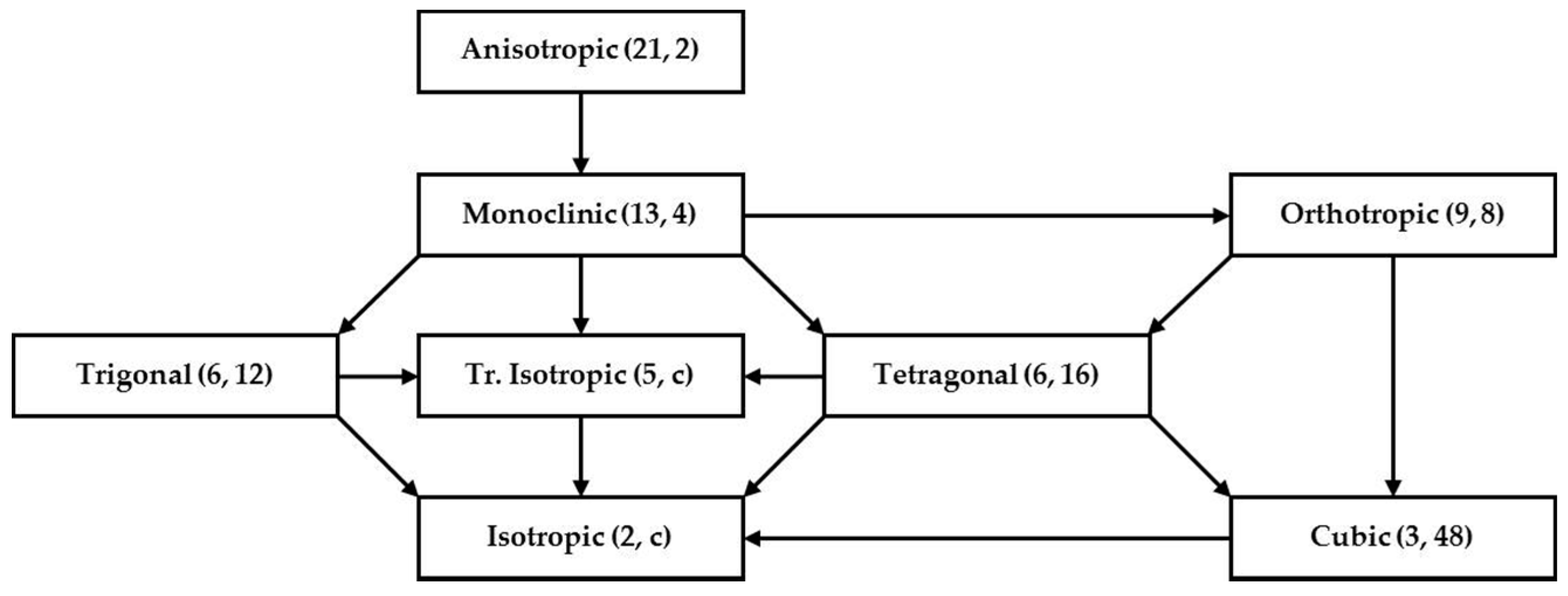
Figure 2.
Dimensionless MEs in the isotropic class with respect to the elasticity tensors of random realizations of polycrystalline copper aggregates with uniformly distributed orientations versus the number of crystallites: (a) ; (b) .
Figure 2.
Dimensionless MEs in the isotropic class with respect to the elasticity tensors of random realizations of polycrystalline copper aggregates with uniformly distributed orientations versus the number of crystallites: (a) ; (b) .

Figure 3.
Regressions for mean dimensionless MEs in the isotropic class as functions of the number of crystallites with respect to the elasticity tensors of random polycrystalline aggregates with uniformly distributed orientations: (a) ; (b) .
Figure 3.
Regressions for mean dimensionless MEs in the isotropic class as functions of the number of crystallites with respect to the elasticity tensors of random polycrystalline aggregates with uniformly distributed orientations: (a) ; (b) .

Figure 4.
Changes in the DPFs (projecting along ) of the polycrystalline copper aggregate during the simple shear test: (a) <111>; (b) <110>; (c) <100>.
Figure 4.
Changes in the DPFs (projecting along ) of the polycrystalline copper aggregate during the simple shear test: (a) <111>; (b) <110>; (c) <100>.
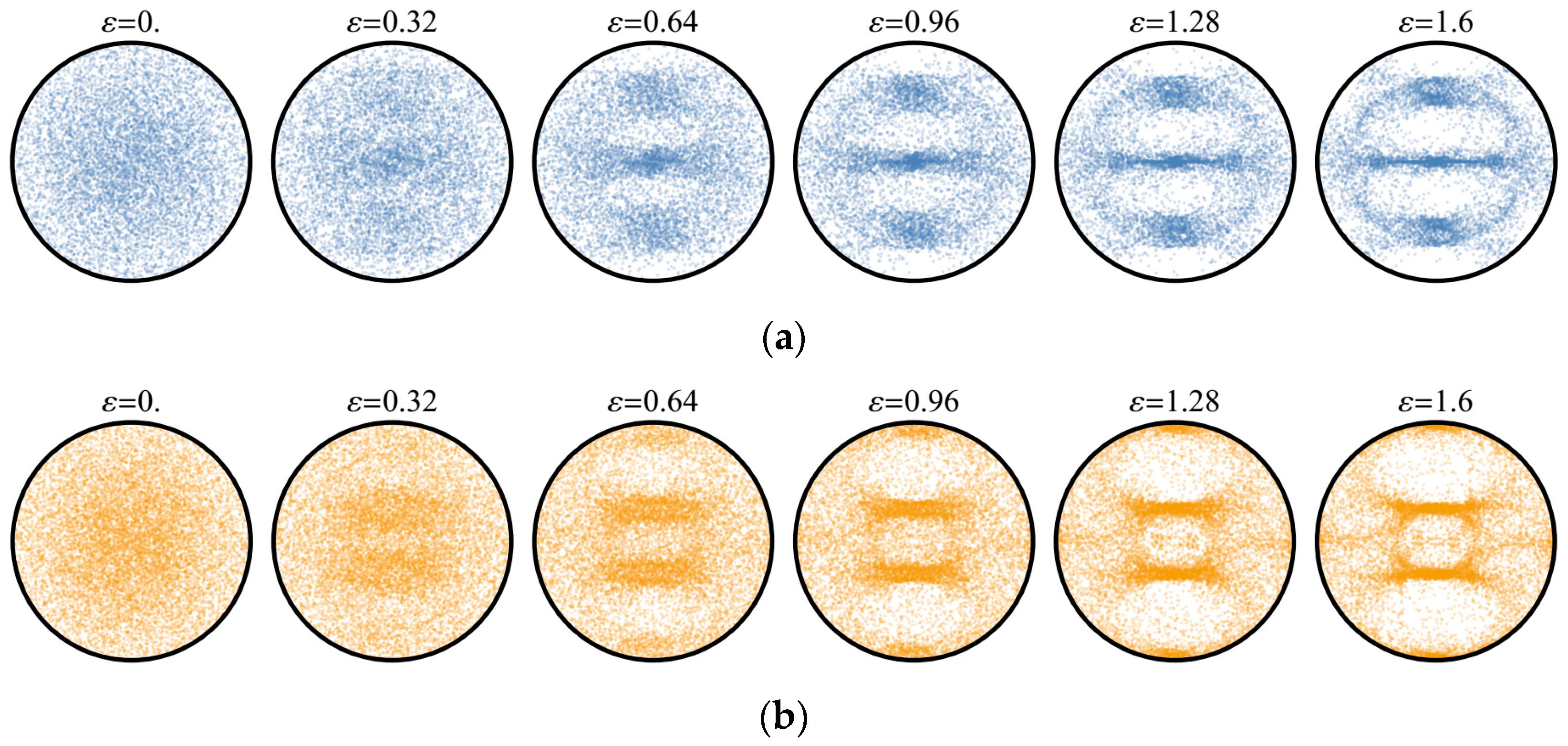
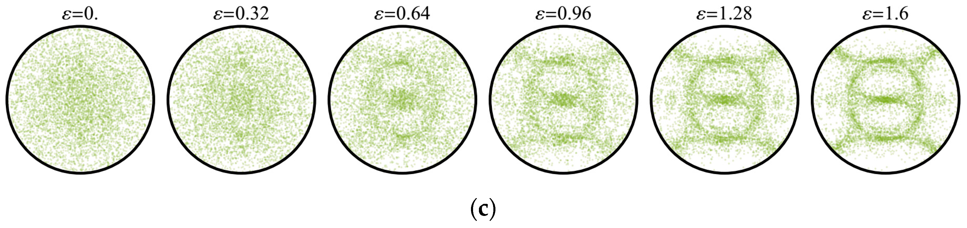
Figure 5.
Changes in the elastic symmetry properties of the polycrystalline copper aggregate during the simple shear test: (a) RMEs in the isotropic class; (b) .
Figure 5.
Changes in the elastic symmetry properties of the polycrystalline copper aggregate during the simple shear test: (a) RMEs in the isotropic class; (b) .
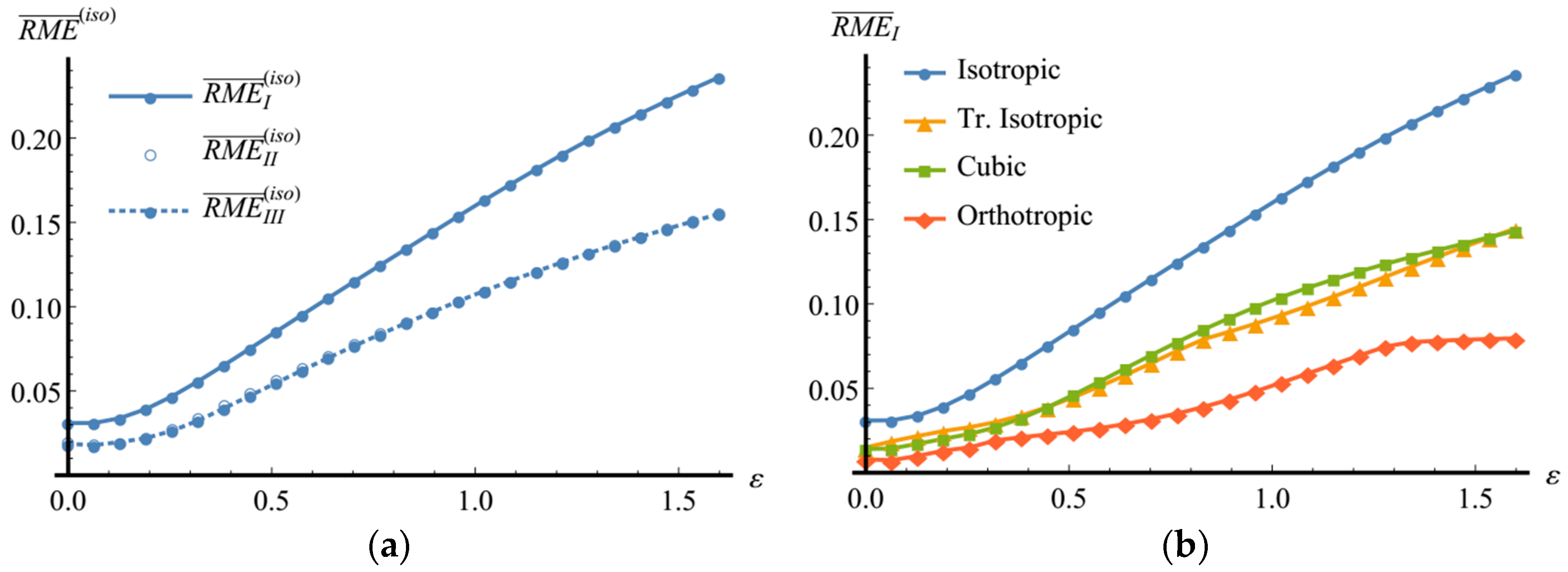
Figure 6.
Changes in the -optimal approximation orientation parameters and the corresponding values of for the elasticity tensor of the polycrystalline copper aggregate during the simple shear test.
Figure 6.
Changes in the -optimal approximation orientation parameters and the corresponding values of for the elasticity tensor of the polycrystalline copper aggregate during the simple shear test.


Figure 7.
Changes in the minimal non-zero Eigen-value of the elasticity tensor of the polycrystalline copper aggregate during the simple shear test.
Figure 7.
Changes in the minimal non-zero Eigen-value of the elasticity tensor of the polycrystalline copper aggregate during the simple shear test.

Figure 8.
Changes in the DPFs (projecting along ) of the polycrystalline copper aggregate during the quasi-axial tension test: (a) <111>; (b) <110>; (c) <100>.
Figure 8.
Changes in the DPFs (projecting along ) of the polycrystalline copper aggregate during the quasi-axial tension test: (a) <111>; (b) <110>; (c) <100>.
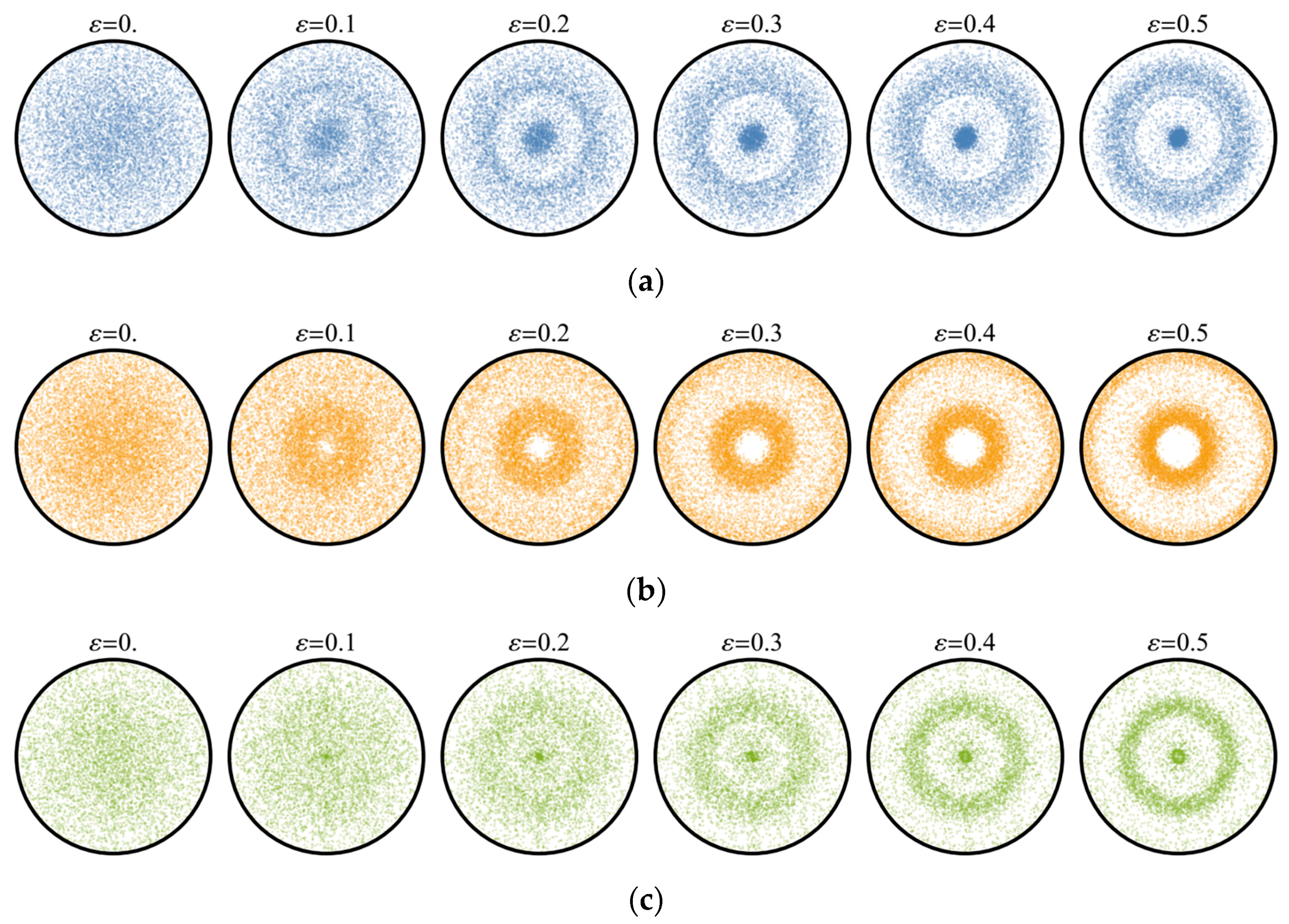
Figure 9.
Changes in the elastic symmetry properties of the polycrystalline copper aggregate during the quasi-axial tension test: (a) RMEs in the isotropic class; (b) .
Figure 9.
Changes in the elastic symmetry properties of the polycrystalline copper aggregate during the quasi-axial tension test: (a) RMEs in the isotropic class; (b) .
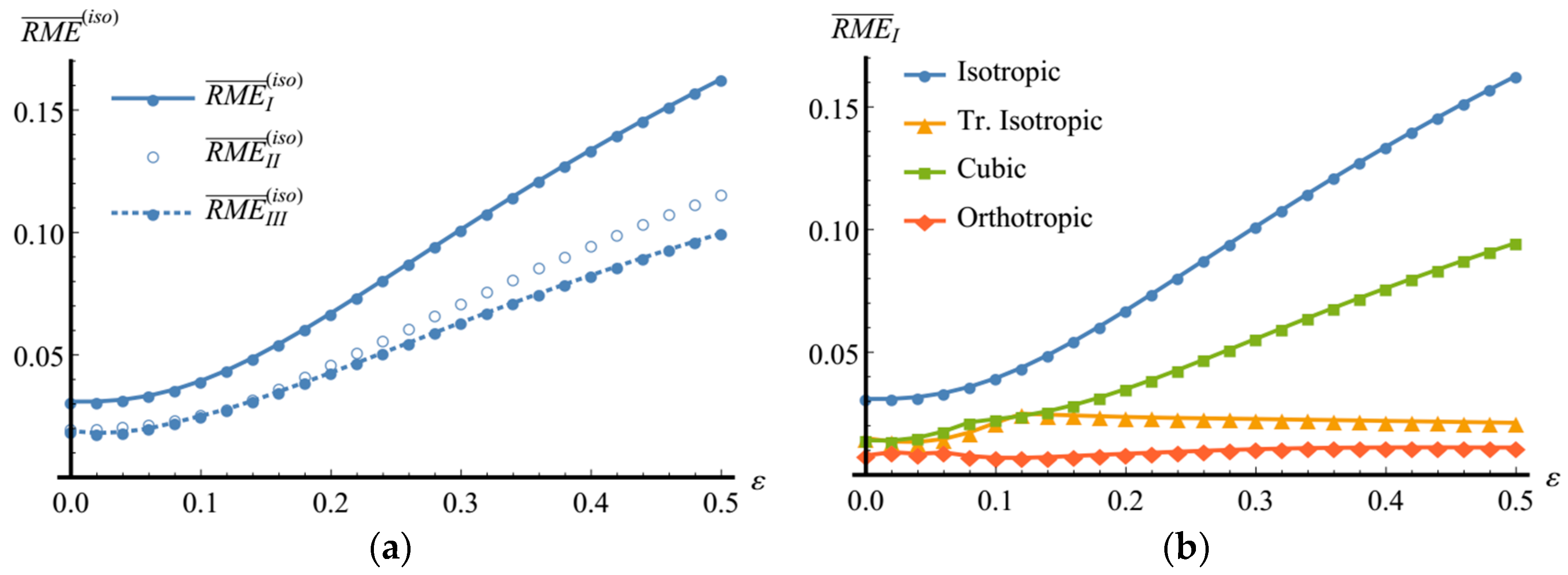
Figure 10.
Changes in the -optimal approximation orientation parameters and the corresponding values of for the elasticity tensor of the polycrystalline copper aggregate during the quasi-axial tension test.
Figure 10.
Changes in the -optimal approximation orientation parameters and the corresponding values of for the elasticity tensor of the polycrystalline copper aggregate during the quasi-axial tension test.

Figure 11.
Changes in the minimal non-zero Eigen-value of the elasticity tensor of the polycrystalline copper aggregate during the quasi-axial tension test.
Figure 11.
Changes in the minimal non-zero Eigen-value of the elasticity tensor of the polycrystalline copper aggregate during the quasi-axial tension test.
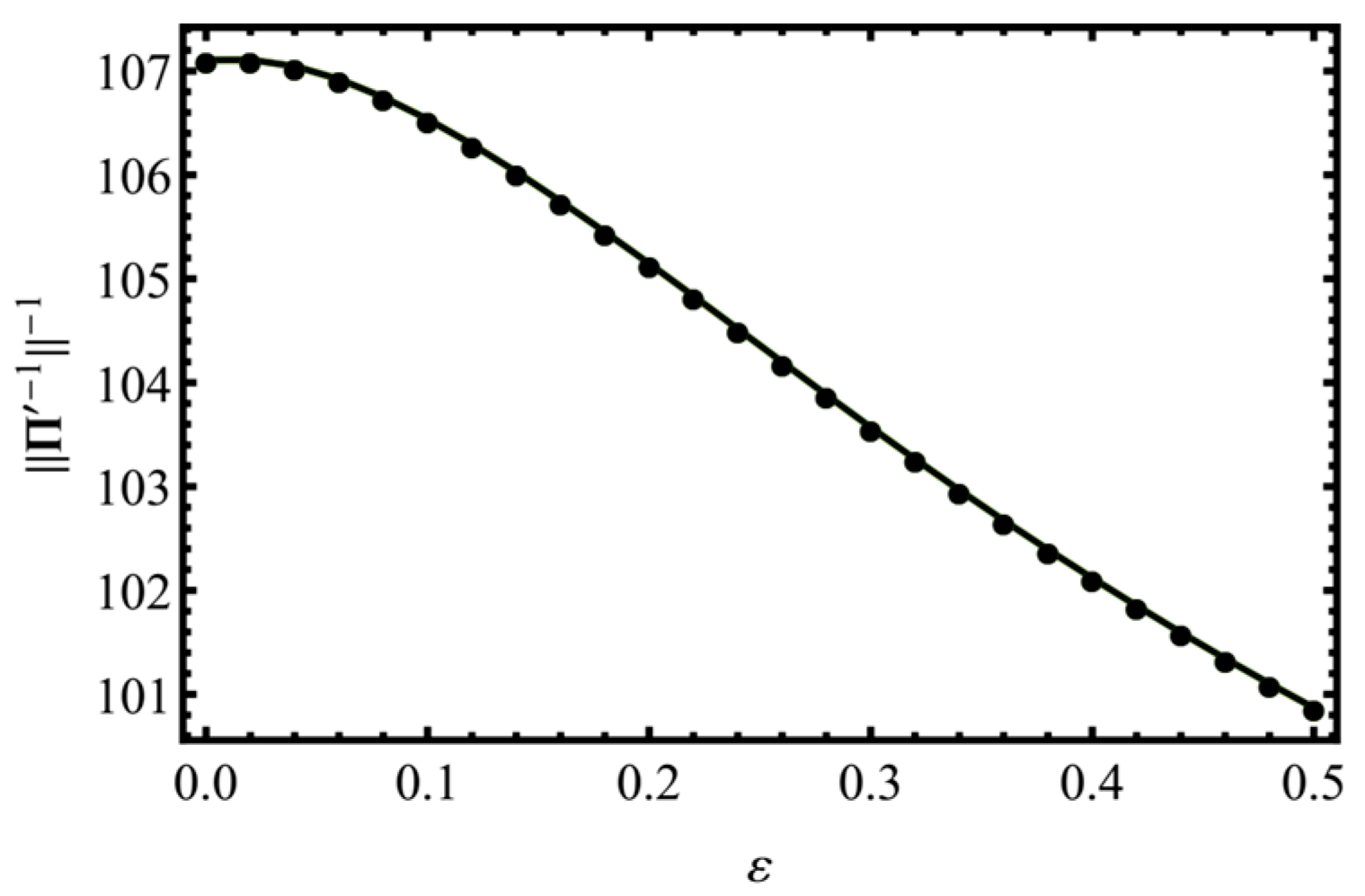
Figure 12.
Changes in the DPFs (projecting along ) of the polycrystalline copper aggregate during the quasi-axial upsetting test: (a) <100>; (b) <110>; (c) <111>.
Figure 12.
Changes in the DPFs (projecting along ) of the polycrystalline copper aggregate during the quasi-axial upsetting test: (a) <100>; (b) <110>; (c) <111>.
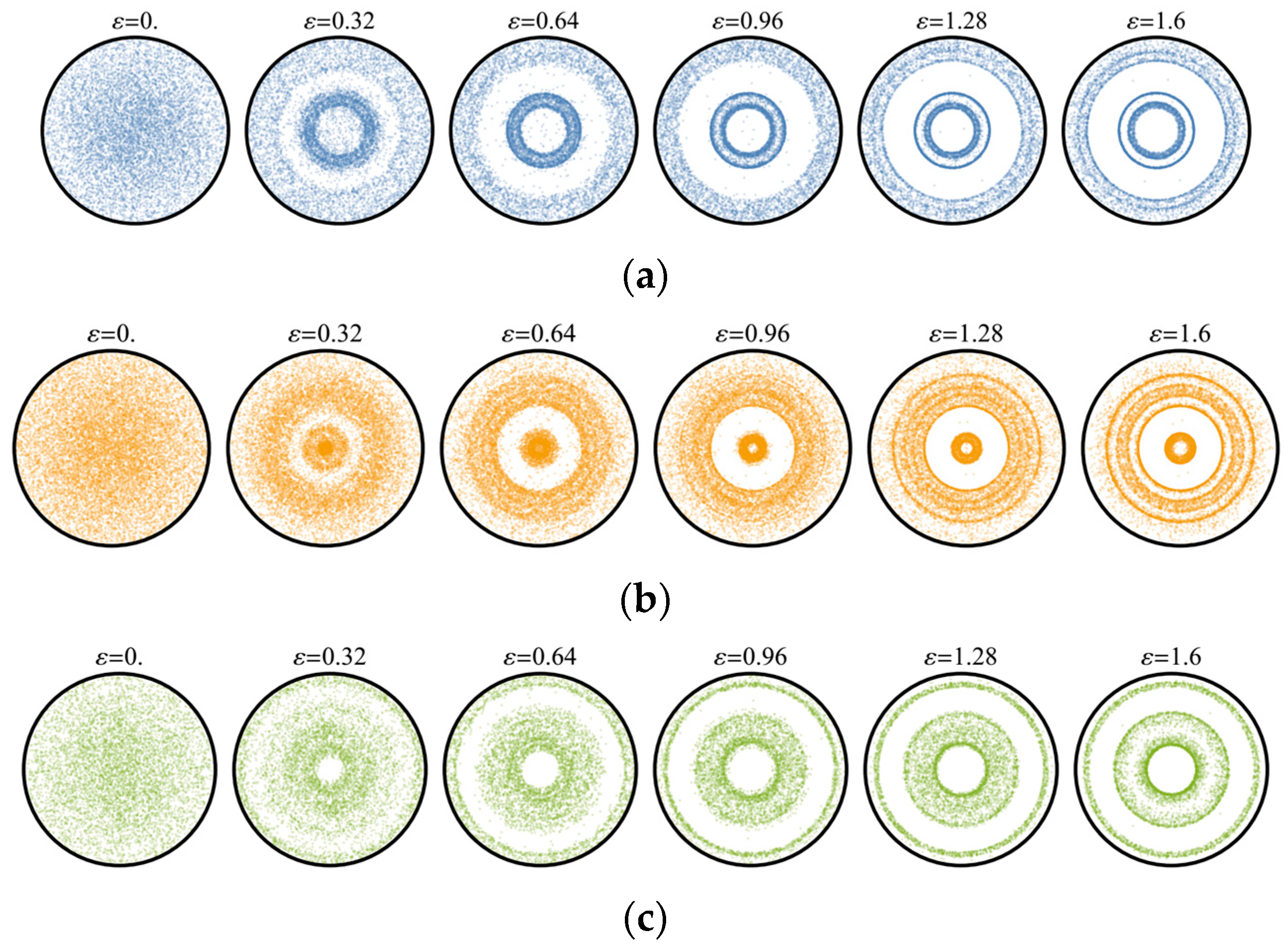
Figure 13.
Changes in the elastic symmetry properties of the polycrystalline copper aggregate during the quasi-axial upsetting test: (a) RMEs in the isotropic class; (b) .
Figure 13.
Changes in the elastic symmetry properties of the polycrystalline copper aggregate during the quasi-axial upsetting test: (a) RMEs in the isotropic class; (b) .

Figure 14.
Changes in the -optimal approximation orientation parameters and the corresponding values of for the elasticity tensor of the polycrystalline copper aggregate during the quasi-axial upsetting test.
Figure 14.
Changes in the -optimal approximation orientation parameters and the corresponding values of for the elasticity tensor of the polycrystalline copper aggregate during the quasi-axial upsetting test.
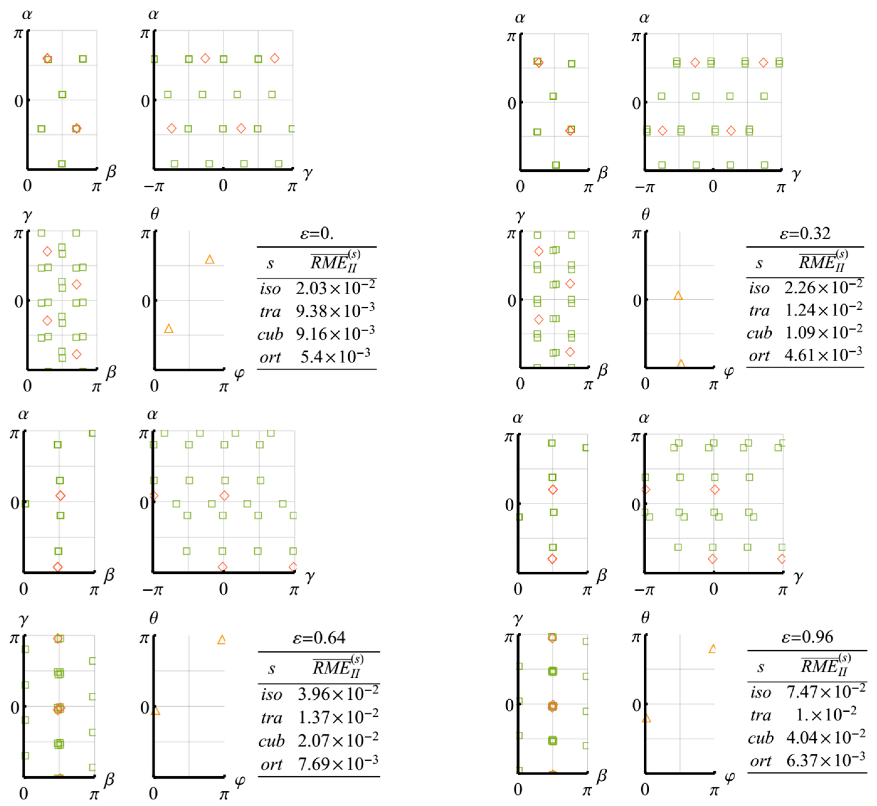

Figure 15.
Changes in the minimal non-zero Eigen-value of the elasticity tensor of the polycrystalline copper aggregate during the quasi-axial upsetting test.
Figure 15.
Changes in the minimal non-zero Eigen-value of the elasticity tensor of the polycrystalline copper aggregate during the quasi-axial upsetting test.


Table 1.
The structure of base tensors for some symmetry classes.
| Symmetry Class () | Elastic Modulus Index () | Non-Zero Components of in Canonical Basis | |
|---|---|---|---|
| Indexes | Value | ||
| Isotropic | 1122 | 1111, 1122, 1133,2211, 2222, 2233,3311, 3322, 3333 | 1 |
| 1212 | 1212, 1221, 1313, 1331,2112, 2121, 2323, 2332,3113, 3131, 3223, 3232 | 1 | |
| 1111, 2222, 3333 | 2 | ||
| Transversely Isotropic | 1111 | 1212, 1221, 2112, 2121 | 0.5 |
| 1111, 2222 | 1 | ||
| 1122 | 1212, 1221, 2112, 2121 | –0.5 | |
| 1122, 2211 | 1 | ||
| 1133 | 1133, 2233, 3311, 3322 | 1 | |
| 2323 | 1212, 1221, 1313, 1331,2112, 2121, 3113, 3131 | 1 | |
| 3333 | 3333 | 1 | |
| Cubic | 1111 | 1111, 2222, 3333 | 1 |
| 1122 | 1122, 1133, 2211, 2233, 3311, 3322 | 1 | |
| 1212 | 1212, 1221, 1313, 1331,2112, 2121, 2323, 2332,3113, 3131, 3223, 3232 | 1 | |
| Orthotropic | 1111 | 1111 | 1 |
| 1122 | 1122, 2211 | 1 | |
| 1133 | 1133, 3311 | 1 | |
| 1212 | 1212, 1221, 2112, 2121 | 1 | |
| 1313 | 1313, 1331, 3113, 3131 | 1 | |
| 2222 | 2222 | 1 | |
| 2233 | 2233, 3322 | 1 | |
| 2323 | 2323, 2332, 3223, 3232 | 1 | |
| 3333 | 3333 | 1 | |
Table 2.
MEs for numerically optimized class approximations.
| Notation | Expression | Minimized Objective |
|---|---|---|
Table 3.
Regression parameters for mean dimensionless MEs in the isotropic class as functions of the number of crystallites with respect to the elasticity tensors of random polycrystalline aggregates with uniformly distributed orientations.
Table 3.
Regression parameters for mean dimensionless MEs in the isotropic class as functions of the number of crystallites with respect to the elasticity tensors of random polycrystalline aggregates with uniformly distributed orientations.
| Crystal | Elastic Moduli, GPa | ||||||||
|---|---|---|---|---|---|---|---|---|---|
| Transversely Isotropic Elasticity | |||||||||
| Mg | 59.7 | 26.2 | 16.4 | 21.7 | 61.7 | 0.22 | 0.50 | 0.19 | 0.55 |
| -Ti | 162.4 | 92.0 | 46.7 | 69.0 | 180.7 | 0.52 | 0.51 | 0.36 | 0.54 |
| Zn | 161.0 | 34.2 | 38.3 | 50.1 | 61.0 | 3.08 | 0.51 | 2.36 | 0.54 |
| Cubic Elasticity | |||||||||
| Al | 108.4 | 62.3 | 28.5 | - | - | 0.26 | 0.51 | 0.14 | 0.48 |
| Cu | 168.4 | 121.4 | 75.4 | - | - | 2.42 | 0.51 | 1.36 | 0.48 |
| -Fe | 287.0 | 141.0 | 116.0 | - | - | 0.65 | 0.50 | 0.35 | 0.47 |
Table 4.
Crystallite mutual orientations in the polycrystalline copper aggregates with the most - isotropic elastic properties.
Table 4.
Crystallite mutual orientations in the polycrystalline copper aggregates with the most - isotropic elastic properties.
| Optimal Mutual Orientations | DPFs (Projecting along ) | , GPa | ||||
|---|---|---|---|---|---|---|
| <111> | <110> | <100> | ||||
| 2 |  |  |  |  | 57.897 | 0.710 |
| 3 |  |  |  |  | 18.951 | 0.192 |
| 4 1 |  |  |  |  | 0 | 0 |
1 The general case is considered in [78].
© 2017 by the authors. Licensee MDPI, Basel, Switzerland. This article is an open access article distributed under the terms and conditions of the Creative Commons Attribution (CC BY) license (http://creativecommons.org/licenses/by/4.0/).
Share and Cite
MDPI and ACS Style
Trusov, P.V.; Ostapovich, K.V. On Elastic Symmetry Identification for Polycrystalline Materials. Symmetry 2017, 9, 240. https://doi.org/10.3390/sym9100240
AMA Style
Trusov PV, Ostapovich KV. On Elastic Symmetry Identification for Polycrystalline Materials. Symmetry. 2017; 9(10):240. https://doi.org/10.3390/sym9100240
Chicago/Turabian StyleTrusov, Peter V., and Kirill V. Ostapovich. 2017. "On Elastic Symmetry Identification for Polycrystalline Materials" Symmetry 9, no. 10: 240. https://doi.org/10.3390/sym9100240
Note that from the first issue of 2016, this journal uses article numbers instead of page numbers. See further details here.