Multi-Objective Optimization Algorithm Based on Sperm Fertilization Procedure (MOSFP)


Department of Computer System and Technology, Faculty of Computer Science and Information Technology, University of Malaya, Kuala Lumpur 50603, Malaysia
*
Author to whom correspondence should be addressed.
Symmetry 2017, 9(10), 241; https://doi.org/10.3390/sym9100241
Submission received: 7 September 2017
/
Revised: 11 October 2017
/
Accepted: 12 October 2017
/
Published: 20 October 2017
Abstract
:In this paper, we propose an extended multi-objective version of single objective optimization algorithm called sperm swarm optimization algorithm. The proposed multi-objective optimization algorithm based on sperm fertilization procedure (MOSFP) operates based on Pareto dominance and a crowding factor, that crowd and filter out the list of the best sperms (global best values). We divide the sperm swarm into three equal parts, after that, different types of turbulence (mutation) operators are applied on these parts, such as uniform mutation, non-uniform mutation, and without any mutation. Our algorithm is compared against three well-known algorithms in the field of optimization. These algorithms are NSGA-II, SPEA2, and OMOPSO. These algorithms are compared using a very popular benchmark function suites called Zitzler-Deb-Thiele (ZDT) and Walking-Fish-Group (WFG). We also adopt three quality metrics to compare the convergence, accuracy, and diversity of these algorithms, including, inverted generational distance (IGD), spread (SP), and epsilon (). The experimental results show that the performance of the proposed MOSFP is highly competitive, which outperformed OMOPSO in solving problems such as ZDT3, WFG5, and WFG8. In addition, the proposed MOSFP outperformed both of NSGA-II or SPEA2 algorithms in solving all the problems.
1. Introduction
The use of evolutionary algorithms in the area of multi-objective optimization has significantly grown in the last decades. Evolutionary multi-objective optimization (EMO) is giving rise to a wide variety of optimization algorithms. These algorithms use a set of techniques including, dominated tree [1], adaptive grid based on data structures to store non-dominated vectors [2], and archive techniques, etc. These techniques help different types of algorithms to provide a solution for various multi-objective optimization problems (MOOPs) [3]. Multi-objective optimization (MOO) is a concept based on plurality of objective functions, rather than single objective optimization (SOO) that is used to solve a single objective function. These functions in MOO are often conflicting and non-commensurable with each other. Based on this observation, the Pareto optimality concept has been introduced to solve the problems of MOO instead of using the optimality concept of SOO, where the final solutions of MOO problems have been selected among a set of Pareto optimal solutions [4].
Based on the idea of Pareto optimality, there are many single optimization algorithms that have been extended to work on MOO problems, which some of these algorithms inspired from the metaphor of natural or man-made processes [5]. Examples of these algorithms are genetic algorithm (GA) and particle swarm optimization (PSO) [6,7]. Non-dominated sorting genetic algorithm (NSGA) [8] and non-dominated sorting genetic algorithm II (NSGA-II) [9] are the extended versions of GA that are used to optimize different types of MOO problems. In addition, multi-objective particle swarm optimization (MOPSO) and optimized multi-objective particle swarm optimization (OMOPSO) are the extended versions of PSO algorithms, which are created to solve MOO problems [10,11].
These algorithms are used to find a solution for a wide variety of real world multi-objective optimization problems (MOOPs). Examples of these problems include the Yagi–Uda antenna design [12], the design of mobile and telecommunication networks [13], scheduling [14], rock crusher design [15], stationary gas turbine combustion process optimization [16], nuclear fuel management [17], defense applications [18], and distributing products through oil pipeline networks [19]. These problems have many objectives, some of them are minimization and the other are maximization objectives. Usually, there is a set of compromise solutions, and a trade-off between these objectives, so the aim of the multi-objective optimization algorithm (MOOA) is to discover a range of solutions that offer a variety of tradeoffs between these objectives [20].
Sperm swarm optimization (SSO) algorithm is a recent heuristic inspired by the fertilization procedure, in which sperms swim in swarms until reaching the waited egg in the fallopian tubes. SSO has been found to provide a solution for a wide variety of optimization tasks [21], but until recently it had not been extended to deal with multiple objectives. SSO seems particularly appropriate for MOO tasks mainly because of the high speed of convergence and good quality of solutions that the algorithm presents for SOO [21]. For this purpose, in this paper, we intend to extend the SSO as MOOA, which we will compare it with different types of MOOAs by using a set of quality metrics, such as inverted generational distance (IGD), spread (SP), and epsilon (). These metrics are measured based on the results of some benchmarks functions, such as Zitzler-Deb-Thiele (ZDT) and Walking-Fish-Group (WFG) test suites that will be discussed further in later Sections. We organize this paper as follows: Section 2 presents state of the art. The proposed multi-objective optimization algorithm based on sperm fertilization procedure (MOSFP) is presented in Section 3. Section 4 describes the details of the comparison strategy. Section 5 shows the experimental test and results. Section 6 presents the discussion and we conclude the work in Section 7.
2. State of the Art
This Section provides a review on SSO algorithm, which covers its parts and limitations. In addition, this Section summarizes the full procedure of the SSO algorithm with its mathematical rules.
Sperm Swarm Optimization Algorithm
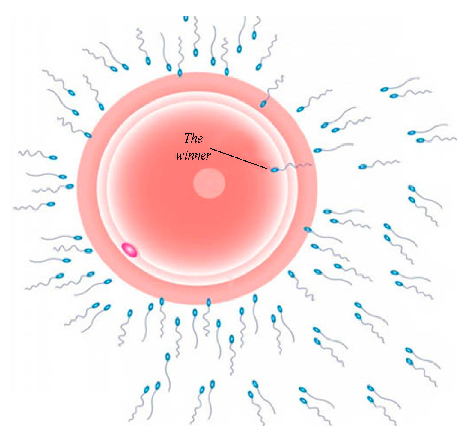
Shehadeh et al. [21], proposed an approach called sperm swarm optimization (SSO), which was inspired by fertilization procedure. This approach can be considered as a distributed behavioral algorithm that can be applied to multi-dimensional search space. Through the simulation, the behavior of motility of each individual can be affected by either the current best local solution or by the best global solution of the sperm swarm. The former solution can be achieved by any sperm based on the certain neighborhood, as each individual remembers its past position to determine the new position. At the same time, the latter solution can be achieved by any sperm based on its position from the target, as this solution will be remarked by the sperm that has a very closest position to the target (egg). In this algorithm, a sperm that has a very closest position to the target is called the winner. Researchers found that the sperm swarms move together, forming groups when they are swimming in viscoelastic fluids and their behavior of moving exhibiting similar to “flocking”. They also observed a certain movement beat and degree of synchronicity of tail movements during grouping [22]. Figure 1 shows the winner and other sperm cells reaching for the egg [21].
The evolutionary algorithms such as GA is an inherently discrete procedure. The enhancement of GA using adaptive selection scheme, such as in [23] is used to deal with each individual independently and can easily perform discrete design variables. Therefore, the static variables can be used easily in their work. However, SSO uses the random parameters rather than static parameters, which play a significant role in updating the position of each sperm until reaching the optimal value.
Most of the previous well-known algorithms use randomness in their evaluations. PSO [7] is one of the most popular algorithms in the field of optimization that uses the randomness in its procedure. C1 and C2 numerical variables, that take random values in the range of 0 to 4. The adaptiveness of the SSO algorithm is based on two factors (i.e., temperature and pH). These variables take a range of numerical variables randomly based on the following rules:
- The normal pH value of a healthy female reproductive system is around 4.5–5.5 [24]. However, low pH of mucus acidic may destroy and deactivate the motility of sperm. Therefore, during the ovulation, the pH of vaginal acid or acidic is in the range of 7 to 4, which is very appropriate for sperm motility and is considered very alkaline and non-toxic to sperm [25]. The pH value of the female reproductive system is affected by the type of food consumed [26] and emotional or mood status of the female, such as happiness or sadness, etc. [27]. Based on this information, we can estimate that the value of pH will be varied in the range of 7 to 14.
- The temperature of the female reproductive system plays a significant role of determining the sperms movement direction. The scientists found that the sperm head acts like a temperature sensor to search for a warmer area (the egg location) [28]. Furthermore, the sperm head can response and sense to a temperature difference of <0.0006 °C [28]. The temperature inside the vagina can change based on women status. The average temperature inside the vagina is approximately between 35.1 and 37.4 °C [29]. However, this temperature may reach 38.5 °C in some cases due to vaginal blood pressure circulation [30].Based on this information, we can estimate that the value of temperature will be varied in the range of 35.1–38.5.
Based on the previous rules, we can notice that SSO is difference than evaluation algorithms such as GA, in which GA is an inherently discrete procedure. GA and its adaptive methods (enhancement methods of GA using some adaptive selection scheme, etc.), such as in [23], are used to deal with each individual independently; therefore, it easily performs discrete design variables. Therefore, the static variables can be used easily in their evaluation. In a different view, SSO uses the inherently continuous technique to update the sperm velocity and location, which each sperm remembers its past location and based on it produces a new location. SSO uses the random parameter rather than static parameters (i.e., temperature and pH), which play a significant role in updating the position of each sperm until reaching the optimal value. The history of samples is not cached for each sperm such as pH value and the temperature value of the visited area. Only, the position of each sperm will be cached in memory. This is because the position is the outcome of multiplying some numerical variables with each others’, such as the pH value, temperature value, and sperm best solution, etc. Therefore, the position of each sperm is very important to be cached, in which SSO uses the cached position (old position) to compare it with the new position and it changes the old position just in case of if the new position is better than the old one. This is clear in the equations from 1 to 5, and procedure of Algorithm 1. In addition, it uses mutation operations, which are used to increase the convergence. The mathematical rule that is used in SSO to update the sperm velocity consists three parts as follows:
- The initial velocity of the sperm: is the velocity that acquired by each sperm after the ejaculation in the cervix zone. The sperm swarms take random positions inside the cervix and their velocity is affected by the pH value in that position. This velocity can be represented in the following rule:where:
- D: is the velocity damping factor, which is a random number between 0 and 1.
- Vi: is the sperm velocity.
- pH_Rand1: is the pH value, which is a random number in the range of (7, 14).
- Personal sperm current best solution: is the best solution that achieved so far by the sperm. As we mentioned previously, sperm head acts like a temperature sensor, which prefers to swim towards warmer temperatures (egg location) [28]. In addition, sperm moves forward to search on the guidance (higher concentrations of molecules) that produced and released by the egg, which this guidance knew as Chemo-taxis [31]. From this information, we can realize that the sperm will not swim backward to the cervix, but, will go forward towards warmer temperatures (the egg location in fallopian tubes). Based on that, this position can be achieved by comparing the sperm current position on X-axis and Y-axis with a sperm past position that is stored in the memory. The past position can be replaced by the current position if the current position is better than the past position. Personal sperm current best solution can be represented in the following equation:where:
- sb_ solution []: is the best solution that has been achieved so far, which denoted by Sperm Best (sb_ solution).
- pH_Rand2: is the pH value, which is a random number in the range of (7, 14).
- Temp_Rand1: is the area temperature, which is a random number in range (35.1, 38.5).
- Global best value is used to determine which sperm’s data is currently closest to the target (at the end, this sperm will represent as the winner). The value of sperm global best value is represented as the following equation:where:
- sgb_solution[]: is the best solution of any sperm has achieved so far which denoted by Sperm Global Best (sgb_solution).
- pH_Rand3: is the pH value, which is a random number in the range of (7, 14).
- Temp_Rand2: is the area temperature, which is a random number in the range of (35.1, 38.5).
- current[]: is the current best solution represented by the following equation.
where v[] is the sperm velocity which measured by companies the previous velocities in one equation as follows:
We take the log for both pH and temperature parameters to normalize these values to become small values. This will help to achieve an acceptable slow velocity that simulates the normal movements of real sperm.
In this paper, we intend to extend SSO algorithm as a multi objective algorithm using Pareto dominance and the concept of winner. The winner is the nearest sperm to the egg. The value of this sperm is considered as the best value of the swarm. The value of the winner (global best value) is used as a reference for all of the other sperm in the swarm to adjust their velocities on the search space domain. The benefits of MOOA over single objective optimization algorithm (SOOA) is the ability of MOOA in finding the correct trade-off between possibly conflicting terms by providing a set of solutions that explore these trade-offs, so that the optimal choice can be made easily. This helps to utilize SSO algorithm in solving many MOOPs such as the problems that mentioned in the introduction Section. The steps of SSO algorithm procedure can be summarized in Algorithm 1.
| Algorithm 1 Sperm swarm optimization (SSO) |
| 1: Begin |
| 2: Step 1: initialize positions for all sperms. |
| 3: Step 2: for i=1:number of sperm do |
| 4: Step 3: evaluate the fitness for each sperm |
| 5: If obtained fitness > sperm best solution then |
| 6: Set the current value as the sperm best solution |
| 7: End if |
| 8: End for |
| 9: Step 4: choose the sperm global best solution based on the winner. |
| 10: Step 5: for i=1:number of sperm Do |
| 11: Do the swim using velocity update rule |
| 12: Update sperm location on the search space |
| 13: End for |
| 14: Step 6: for i=1:number of sperm Do |
| 15: Apply mutation operation on the sperm value |
| 16: End for |
| 17: Step 7: while maximum iterations not achieved return to step 2 and repeat until reaching the |
| 17: maximum number of iterations. |
| 18: End procedure. |
3. Multi-Objective Optimization Algorithm Based on Sperm Fertilization Procedure (MOSFP)
The main idea of every MOOAs is to find Pareto optimal set. The Pareto optimal set is used to balance the conflicting objectives and manage the trade-offs between them. Vilfredo Pareto (the Italian economist), is the founder of the concept of Pareto optimality, which is conceptualized in his work called manual of political economy (MPE) in 1906 [32]. The Pareto optimality definition based on some basic concepts can be introduced as follows:
- Domination: x1, may dominate a position vector, x2 (x1 < x2), if and only if and for at least one k [33].
- Pareto optimal: A vector F is defined as Pareto-optimal if no vector exists x F such that for at least one . An objective vector is called Pareto optimal if the corresponding vector is the Pareto optimal. The set of the Pareto optimal decision vectors F is denoted by [34].
- F is the Pareto optimal of a position vector if no position vector that dominates it, F. The Pareto optimal solution is non-dominated solution, which not dominated by other solutions [34].
- Pareto optimal set: is a set containing all the Pareto optimal vectors [35].
- Pareto front (PF): is defined as [35].
The first step in any MOOA is to minimize the distance between the true Pareto front and the solutions. To achieve this objective, appropriate fitness functions must be defined. Aggregation based method is a traditional method of assigning fitness function, where a weighted sum of the objective functions is used to define the fitness function [36].
There are many limitations of a classic approach, such as the tendency to be inefficient and very susceptible to precise accumulation of goals [32]. For these reasons, the MOOAs have been proposed by many researchers, including complex methods to obtain optimal weights of the objective function such as neural network [37]. Some of the researchers also proposed the Pareto dominance for fitness assignment, where the fitness is proportional to the dominance rank of solutions. Pareto dominance is used in many algorithms to generate and identify a list of best solutions that are used to solve the MOOPs. MOPSO is considered as one of the popular algorithms that uses this technique [38].
In the proposed MOSFP, the crowding factor [39] has been used to help in building the criterion of a second discrimination (additional to Pareto dominance). This also helps in making a decision about winners that should be reserved when the algorithm executes the maximum list size. In our algorithm, the winner has been chosen based on means of a binary tournament that is related to crowding value of the winners. All of the best values (winners) have been crowded as a set. The size of the set of winners (SoW) is identified, in which the maximum size of them are equal to the size of the population or the swarm. After each generation, the SoW and the corresponding crowding values related to them are updated. In the case of the size of SoW is greater than the maximum defined size, the best winners are defined based on their crowding value, and after that, they are reserved and the others are eliminated.
The crowding factor is used in many types of research such as [11,40,41]. This technique helps to control and manage the winners without requiring any kind of selection criterion. In this algorithm, we propose the use of mutation operations that are used in many optimization algorithms, such as NSGA-II, MOPSO, and OMOPSO [8,10,11]. There are many types of the mutation, such as uniform mutation and non-uniform mutation. The uniform mutation provides a constant of variability range for each decision variable, while in non-uniform mutation, the variability range for each decision variable is not constant. We propose the use of different mutation level by combining both uniform and non-uniform mutations as in [11]. These operators play a significant role by modifying the values of the decision variables of a sperm. In addition, we intend of not using mutation at all in case the previous mutation operations failed to find the proper results, this part of the population (population without mutation) will reserve on good results. In this procedure, the swarms are divided to three equal parts, including, part that will have non-uniform mutation, part will have uniform mutation, and part without any mutation. By using this procedure, the MOSFP can explore uniform, non-uniform mutations search space as the process progresses. Algorithm 2 shows the mutation part of the MOSFP algorithm. As it is clear in Algorithm 2, we take modulus of 3 on the population size to divide the population size into three equal parts. On the first part, we apply non-uniform mutation; on the second part, we apply uniform mutation; while, on the third part, we do not apply any mutation at all. We use the concept dominance that has been used in [11,42,43]. This concept is used to fix the size of non-dominance solutions (external archive). We can say that a decision vector x1 dominance a decision vector x2 for some if and only if: and for at least . value is a user defined value, which is used to determine the size of the final external archive. In our algorithm like [11], we use the same value of for all objective functions, which are changed based on the amount of points in the final Pareto front.
| Algorithm 2 Mutation |
| 1: Begin |
| 2: Step 1: for i = 0 to population size do |
| 3: If (i % 3 == 0) then |
| 4: Sperms_ mutated with a non-uniform mutation operator |
| 5: Else if (i % 3 == 1) then |
| 7: Sperms_ mutated with a uniform mutation operator |
| 8: Else |
| 9: Sperms_ without mutation |
| 10: End if |
| 11: End for |
| 12: End procedure. |
The full procedure of MOSFP is summarized in Algorithm 3. At the beginning of the procedure, MOSFP initializes the sperm swarm. SoW is introduced based on the non-dominated sperms. In addition, the crowding factor, later on will be calculated. At each generation, for each sperm, the swim and the mutation procedure that is described in Algorithm 2 have been performed. In order to perform the swim of each sperm, the following equation (sperm velocity update rule) has been used:
where D is a velocity damping factor, which takes a random value in the range of (0, 1); pH_Rand1, pH_Rand2, and pH_Rand3 are the pH values of the visited regions, which take a value in the range of (7, 14). The process of updating the personal sperm current best solution is based on two cases; first, if the value of personal sperm current best solution is dominated by the new sperm; second, if the personal sperm current best solution with the new sperm value are non-dominated with respect to each other. Later on, if all sperms have been updated, the SoW will be updated too, which the sperms that achieve the new positions that are better than the old positions will have the possibility to join the winner set. After that, the will take the place on the procedure to be updated. Finally, the crowding values of SoW are processed to be updated, as many of the winners are eliminated in case of exceeding the determined size of the winners set. This process is repeated many times until it reached the determined number of iterations (imax). The parameter needed by this algorithm are (1) S_size (swarm size), (2) i (number of iterations), (3) mutRate (mutation rate, which is automatically computed), and (4) , which is the value of the bounding size of the .
| Algorithm 3 Multi-objective optimization algorithm based on sperm fertilization procedure (MOSFP) |
| 1: Begin |
| 2: Step 1: initialize positions for all sperms. |
| 3: Step 2: initialize Winners. |
| 4: Step 2: archive the Winners in |
| 5: Step 3: crowd the winners using crowding operation. |
| 6: Step 4: define counter (i) and define number of maximum iterations (iMax). |
| 7: Step 5: do //this do is a do - while |
| 8: For <each sperm> do |
| 9: Select winner from the sperm swarm |
| 10: Update sperms positions using the predefined sperm velocity update rule (perform swim) |
| 11: Perform mutation procedure (Algorithm 1) |
| 12: Evaluate the fitness for each sperm |
| 13: Update personal sperm current best solution |
| 14: End for |
| 15: Update Set of Winners (SoW) |
| 16: Archive winner in |
| 17: Crowd the SoW using crowding operation |
| 18: Update value of counter (i) |
| 19: Step 6: While i < iMax |
| 20: Step 7: archive results in |
| 21: End procedure. |
4. Comparison Strategy
Several test functions have been used to compare our algorithm with the mostly used MOOAs. In order to apply the quantitative assessment of the efficiency and performance of MOOA, three issues should be taken into consideration [38,44].
- Minimize the distance between the global Pareto front (the well-known Pareto front of any problem) and the Pareto front that produced by our approach.
- Maximize the spread of the solutions that produced by our approach, so uniform distribution of vectors can be achieved.
- Maximize the convergence of algorithm to obtain a good quality of the Pareto optimal set found.
Based on these notions, we can apply one metric to estimate each of the three issues previously mentioned. We chose the frequently used metrics for this purpose as in [38,44,45]. These metrics are inverted generational distance (IGD), which is used to cover the notion number 1, spread (SP), which is used to cover notion number 2, and epsilon (), which is used to cover notion number 3. These metrics that adopted in this test are summarized in the following points:
Inverted Generational Distance (IGD): the generational distance measurement was proposed by Van Veldhuizen et al. [46,47,48]. This measurement is used to estimate how far the Pareto front of an algorithm from the true Pareto front of any problem. This metric can be calculated by:
where n is the number of non-dominated vectors that found by any algorithm, di is the Euclidean distance that measured in object space between the true Pareto front of any problem and the vectors that generated by any algorithm. It is clear that IGD metric should be near or equal to zero. In other meaning, if IGD = 0, all of the elements generated are in the true Pareto front of the problem [49,50]. We use IGD to test the first issue, which is mentioned previously, by comparing a true Pareto front of a problem (the reference Pareto front) with a Pareto front that produced by any algorithm of the same problem.
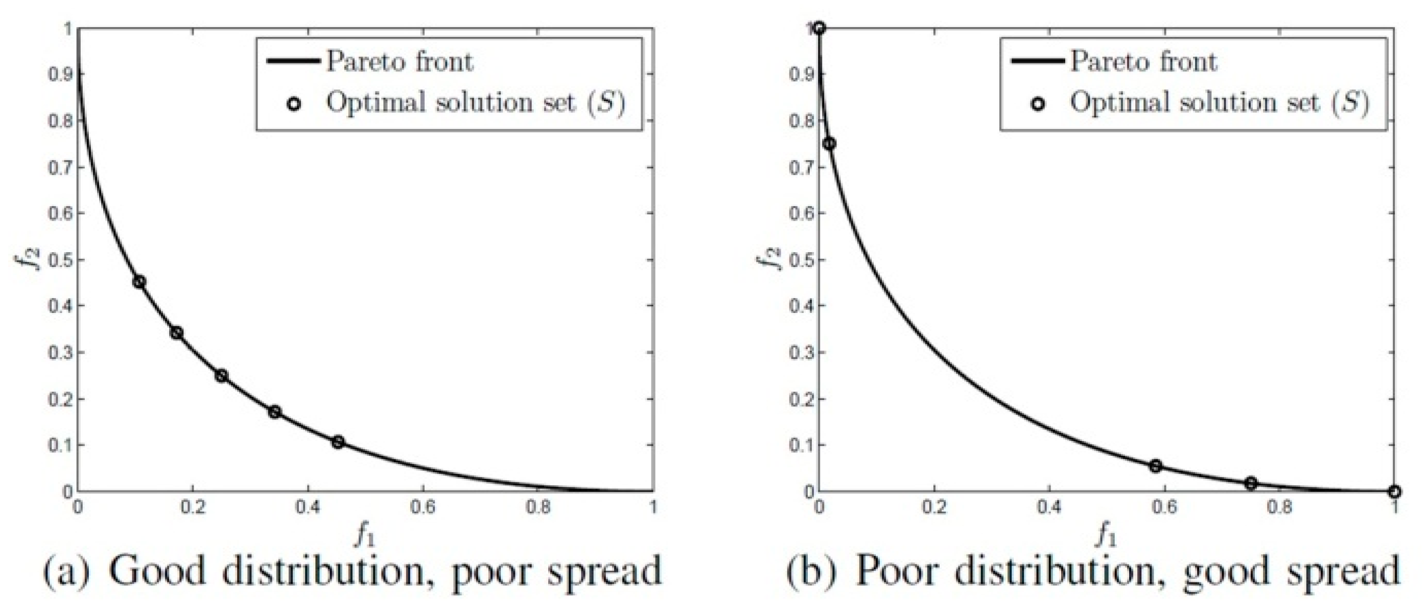
Spread (SP): is the diversity metric that is used to measure the extent of spread and distribution of solutions in the set S of optimal solution. Figure 2 illustrates the spread metric of five non-dominated solutions of S, which are spread in two cases. In the first case shown in Figure 2a, there is a poor spread, but a good distribution, in which S does not contain the radical points, such as (1, 0), (0, 1) on the 2-dimensional Pareto front. On the other hand, in the second case shown in Figure 2b, there is unfavorable distribution, but a good spread of an optimal solution set [51]. We use SP to test the second issue that mentioned previously. SP can be measured by the following equation [52]:
where:
- : is the Euclidean distance measured based on the distance between consecutive solutions,
- : is the average of
- and : are the minimum Euclidean distance measured based on the distance between solutions in S to the radical (bounding) solutions of the Pareto front (P).
Epsilon (): is a binary indicator operates by considering all of the objectives to give a factor by which an approximation set is worse than another. Formally, let M and N be two approximation sets, then equals the minimum factor , which for any solution in set M there is at least one solution in N that is not considered as worse by a factor of considering all the objects [53]. This metric is very important to determine the quality of the obtained solution set by each algorithm [54]. We calculate to test the third issue that mentioned previously.
We chose the previous mentioned metrics as in [38,44,45], which epsilon is used to measure the algorithm convergence, spread is used to measure the spread of the solution, while IGD is a metric that combines both of these components [44].
To estimate the performance of our approach, we choose the most popular MOOAs by consensus of the specialists in the field of MOO. These algorithms are NSGA-II, strength Pareto evolutionary algorithm 2 (SPEA2), and OMOPSO. The study in [54] found that NSGA-II and SPEA2 are the most popular optimization methods among other evolutionary algorithms. Another study in [55] proved that OMOPSO is the most famous optimization approach between other swarm intelligence approaches because it has a higher performance and good quality of results. For these reasons, these algorithms have been chosen to compare their results with MOSFP using the same hardware, environment and platform for each algorithm. We organize these algorithms along with their characteristics as follows:
- Non-dominated Sorting Genetic Algorithm (NSGA-II): is one of the most popular algorithms in MOO area. This algorithm performs a set of operators that deduced from the single objective Genetic Algorithm (GA). These operations are selection, crossover and mutation operators [9]. The pseudo-code of NSGA-II is summarized in Algorithm 4 [8].
Algorithm 4 Non-dominated sorting genetic algorithm II (NSGA-II) 1: Begin 2: Step 1: initialize Population 3: Generate random population – size M 4: Step 2: evaluate objective values 5: Step 3: assign rank (level) based on Pareto dominance-“sort” 6: Step 4: generate child population 7: Step 5: binary tournament selection 8: Step 6: recombination and mutation 9: Step 7: for i=1 to number of generations do 10: With parent and child population 11: Assign rank (level) based on Pareto – “sort” 12: Generate sets on non-dominated fronts 13: Loop (inside) by adding solutions to next generation 14: Starting from the “first” front until M individuals found 15: Determine crowding distances between points on each front 16: Select points (elitist) on the lower front (with lower rank)and are outside a crowding 16: distance 17: Create next generation 18: Binary tournament Selection 19: Recombination and mutation 20: Increment generation index 21: End for 22: End Procedure. - Strength Pareto Evolutionary Algorithm 2 (SPEA2): is a multi-objective algorithm, which is created as an improvement version of strength Pareto evolutionary algorithm (SPEA) algorithm [56]. This algorithm proposed by Zitzler et al. [57]. The procedure of this algorithm works based on dominance, which each single individual dominates or is dominated by other solutions. The nearest neighbor technique is used to guide the search. In addition, this algorithm operates based on preserving the boundary solutions by using archive truncation method [58]. Algorithm 5 summarizes the pseudo-code of this algorithm [59].
Algorithm 5 Strength Pareto evolutionary algorithm 2 (SPEA2) 1: Begin 2: Step 1: initialize population P 3: Step 2: evaluate objective functions 4: Step 3: create external archive A 5: Step 4: for i=1 to number of generations do 6: Compute fitness of individual in P and A 7: Add non-dominated individuals from P and A 8: If capacity of A is exceeded Then 9: Remove individuals from A by truncation operator 10: End If 11: Perform binary tournament selection to create mating pool 12: Perform crossover 13: Perform mutation 14: End for 15: End Procedure. - Optimized Multi-objective Particle Swarm Optimization (OMOPSO): proposed by Sierra et al. [11]. This algorithm performs a set of operators to solve MOOPs, such as crowding the global best solutions that known as leaders, performs mutation, after that, performs an archive of the leaders. The pseudo-code of OMOPSO is summarized in Algorithm 6.In order to compare our algorithm with the previously mentioned algorithms, we use two techniques, including, quantitative and qualitative tests. For the quantitative test, we adopt the IGD, SP, and measures, while for the qualitative test, we compare between the quality of Pareto fronts that is achieved by our algorithm and the Pareto fronts that achieved by the other algorithms. For these purposes, two test suites called Zitzler-Deb-Thiele (ZDT), and Walking-Fish-Group (WFG) have been used in this work.
- Zitzler-Deb-Thiele (ZDT) Test Suite: this suite is proposed by Zitzler et al. [60]. ZDT suite is the most widely utilized suite of benchmark functions in evolutionary algorithms and swarm intelligence algorithms literature. The characteristics of ZDT problems are analyzed in Table 1. From the table, we can notice that the geometry of ZDT1 is convex, and the geometry of ZDT2 is concave. In addition, ZDT3 is disconnected on both the Pareto front and the Pareto optimal set, while the other functions consist of convex or concave components. The ZDT benchmark functions share many characteristics, including, how multimodality can cause a disconnected Pareto problems such as in ZDT3, and many-to-one Pareto problem, such as in ZDT6. These functions utilize only a single parameter, which means that these functions own only one variable. There are many advantages of using ZDT problem as a benchmark function for MOOAs, including, that this suite is well defined and employed in many research papers, which facilitate the comparisons with new MOOA. In addition, the Pareto optimal fronts of this suite are easy to apply and to understand [61]. For these reasons, we choose this suite to test our proposed algorithm.
Algorithm 6 Optimized multi-objective particle swarm optimization (OMOPSO) 1: Begin 2: Step 1: initialize swarm and leaders. Send leaders to 3: Step 2: crowding(leaders), g = 0 4: Step 3: While g < max number of iterations (gmax) 5: For <each particle> do 6: Select leader. Flight. Mutation. Evaluation. Update pbest 7: End for 8: Update leaders, Send leaders to -archive 9: Crowding(leaders), g++ 10: End while 11: Step 4: Report results in -archive 12: End Procedure. - Walking-Fish-Group (WFG) Test Suite: WFG suite consists of nine problems introduced by [62]. The characteristics of these problems are outlined in Table 2 [60]. WFG1 and WFG7 are the only both unimodal and separable. WFG6 and WFG9 are the non-separable reduction problems, and they are more difficult than that of WFG3 and WFG2. WFG4 is a multimodality problem with a large “hill sizes” and it is more difficult than that of WFG9. WFG1 employs different parameters by using dissimilar weights in its variable weighted sum reduction. The parameters of WFG7 are dependent on the position and distance-related parameters, whereas WFG9 is more complex, which its distance-related parameters depend on other distance-related parameters. WFG8 is different than WFG9, wherein its distance-related parameters depend on other position and distance-related parameters. WFG5 is highly deceptive function and can be more difficult than that of WFG9.
The WFG test suite is considered as a comprehensive problem, which consists of a wide range of various problems, including, deceptive problems, a mixed shape Pareto front problems, non-separable problems, a truly degenerate problems, problems with dependencies between both distance and position-related parameters, and problems scalable in the number of position related parameters. The WFG test suite can be considered as one of the most commonly used suite of providing a truer means of estimating the performance of MOOAs [63]. For these reasons, we choose this suite to test our proposed algorithm. The mathematical definition of ZDT and WFG problems has been defined in the Appendix A.
The abbreviation in Table 1 and Table 2 are “NS” for non-separable, “S” for separable, “M” for multimodal, “U” for unimodal, “D” for deceptive. The symbols “✓” and “+” indicate whether a given recommendation is adhered to, whereas the symbols “+” and “−” indicate the presence or absence of some features.
5. Experimental Test and Results
We implement the MOSFP algorithm using jMetal tool in the Java language and integrate the implementation into NetBeans IDE 8.1. All of the tests are carried out on a computer with Intel dual core CPU T3200 and 3 GB RAM running Windows 7. We use standard parameters, as recommended in [63], to compare between the proposed MOSFP algorithm and the other algorithms. These parameters are summarized in Table 3. The parameters of all the algorithms are kept in all of the examples presented next. We report the results obtained from executing 100 independent runs of each algorithm for each test function. In each test function, we set the total number of fitness function evaluations to 5000. Three metrics namely, , SP, and IGD are measured and their best, worst, average, and median of each metric based on 5000 runs are presented.
A. ZDT Test Suites
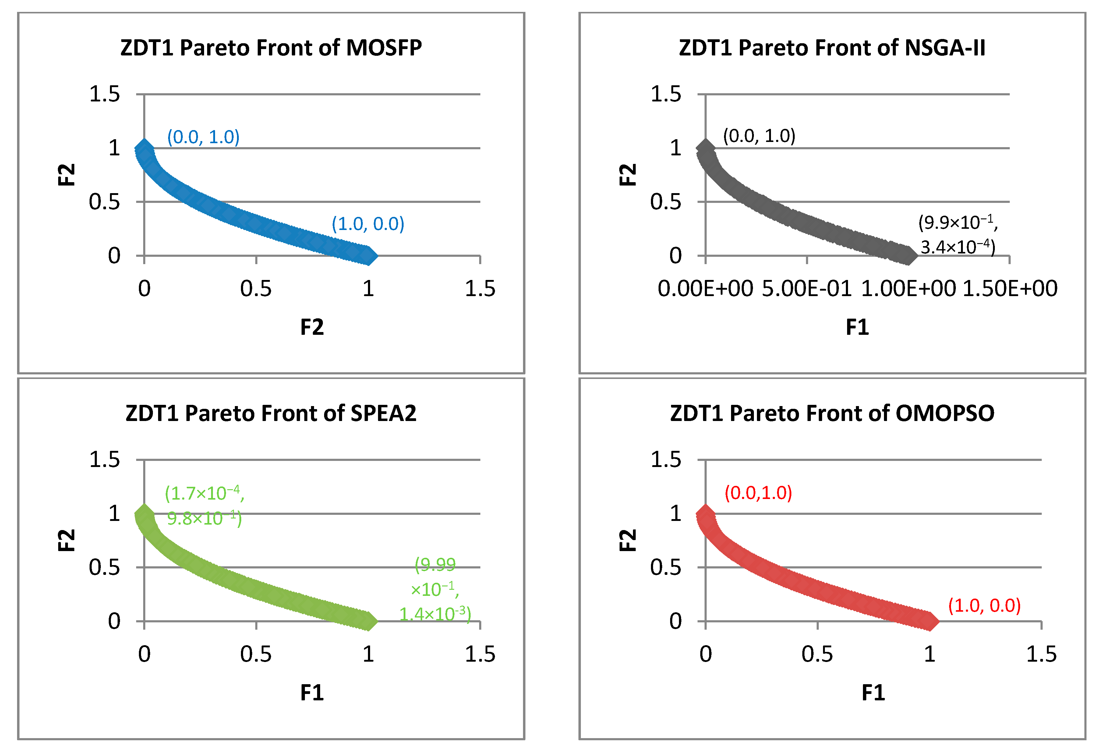
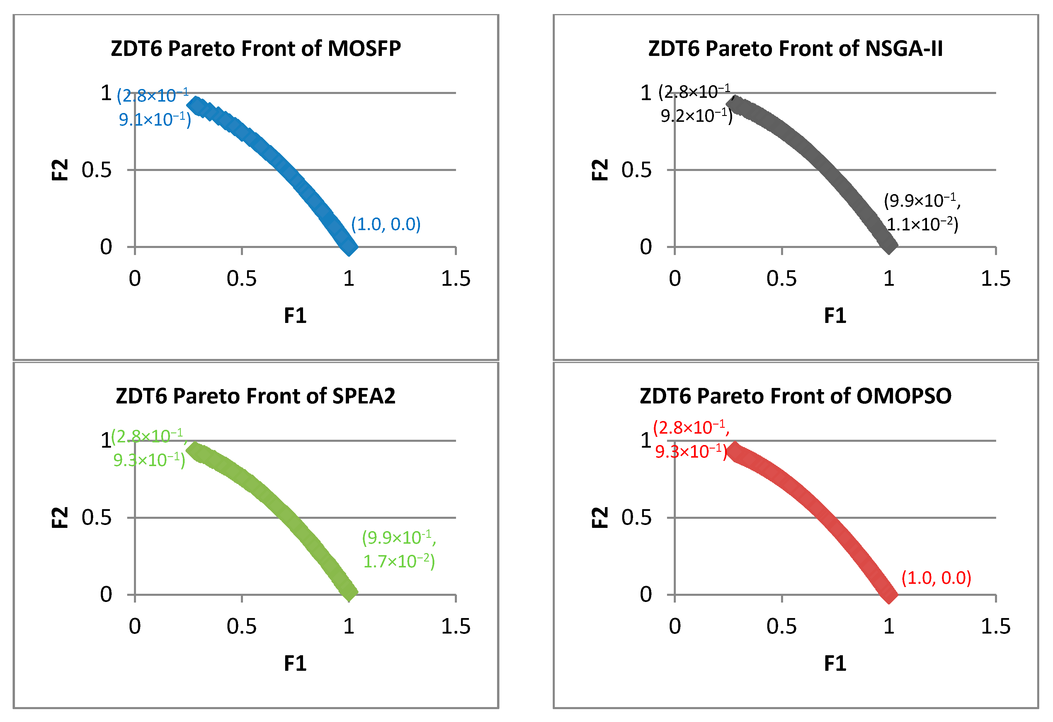
Overall, the OMOPSO algorithm obtained the best average of , SP, and IGD measurement for ZDT test functions, while the proposed MOSFP is in the second followed by NSGA-II and SPEA2 as outlined in Table 4. However, for ZDT3 test function, the proposed MOSFP attained the best average among all of the algorithms. Despite the ranking, the proposed MOSFP has shown a comparable performance with the OMOPSO algorithm as their difference of average , SP, and IGD measurement are minimal. Both the OMOPSO and MOSFP preserved extreme superior points of the Pareto front such as (0, 1) and (1, 0) for ZDT1 and ZDT2 functions as depicted in Figure 3 and Figure 4. Also, both the OMOPSO and MOSFP preserved the Pareto front extreme superior points of (0, 1) for ZDT3 function and (1, 0) for ZDT6 function, as shown in Figure 5 and Figure 6. In opposite, NSGA-II and SPEA2 failed to obtain these optimal extreme values of the Pareto front for all ZDT functions.
B. WFG Test Suites
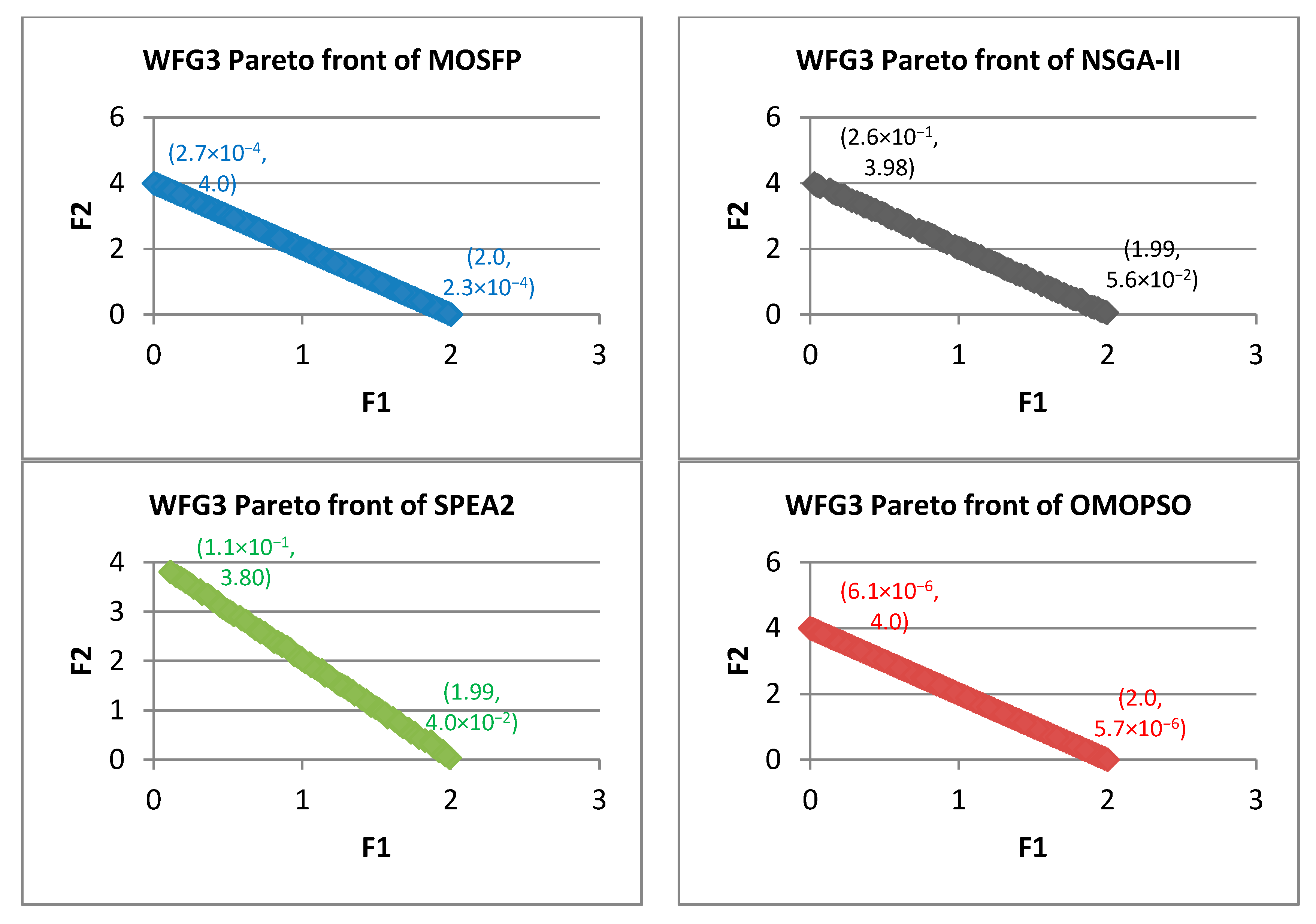
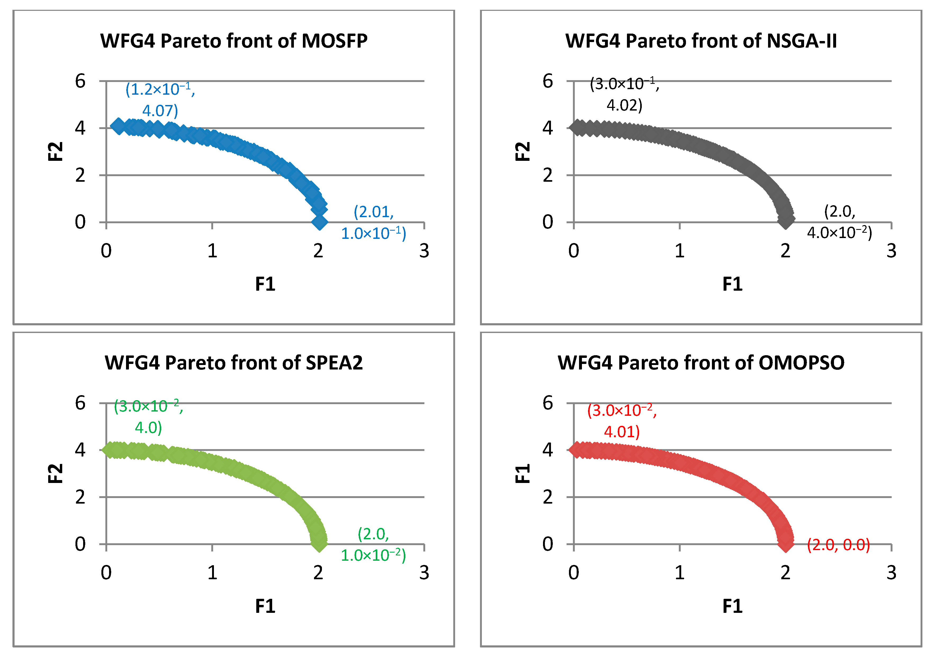
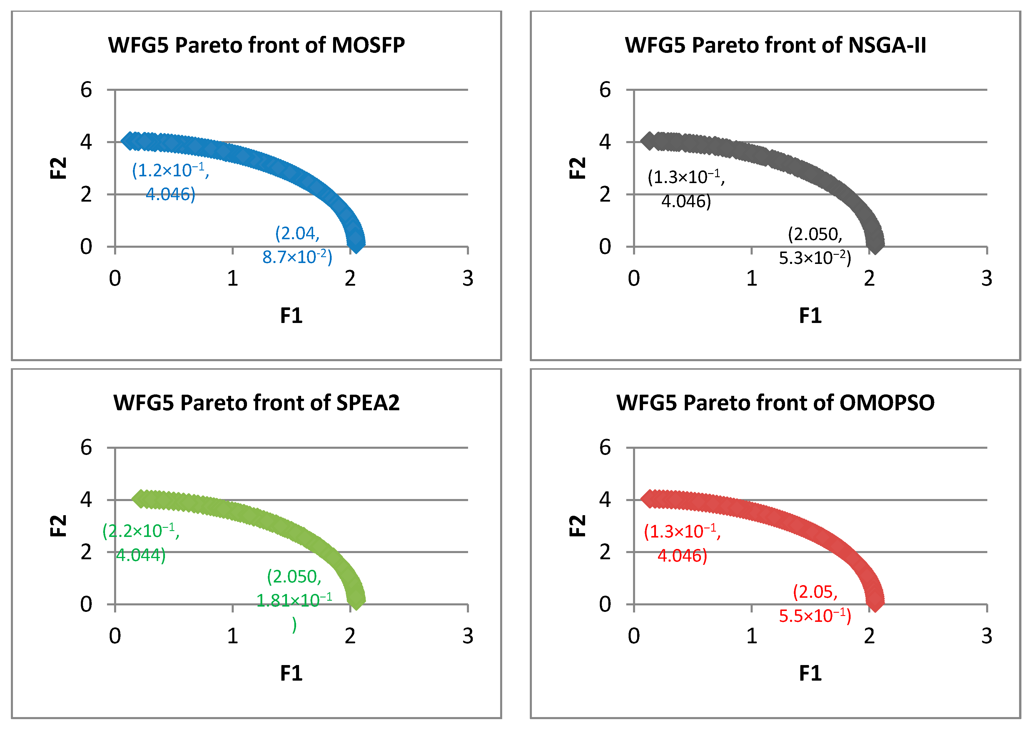
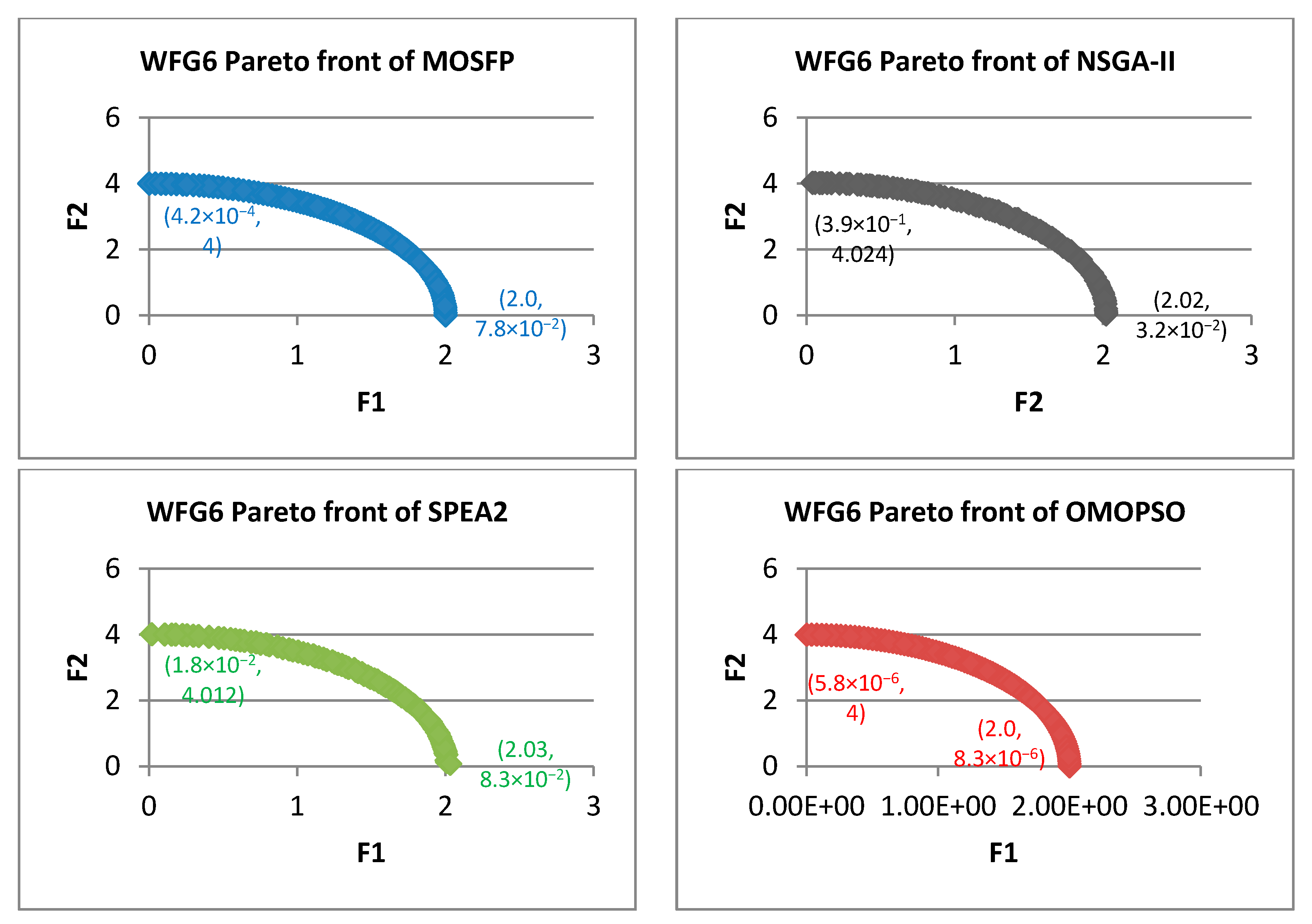
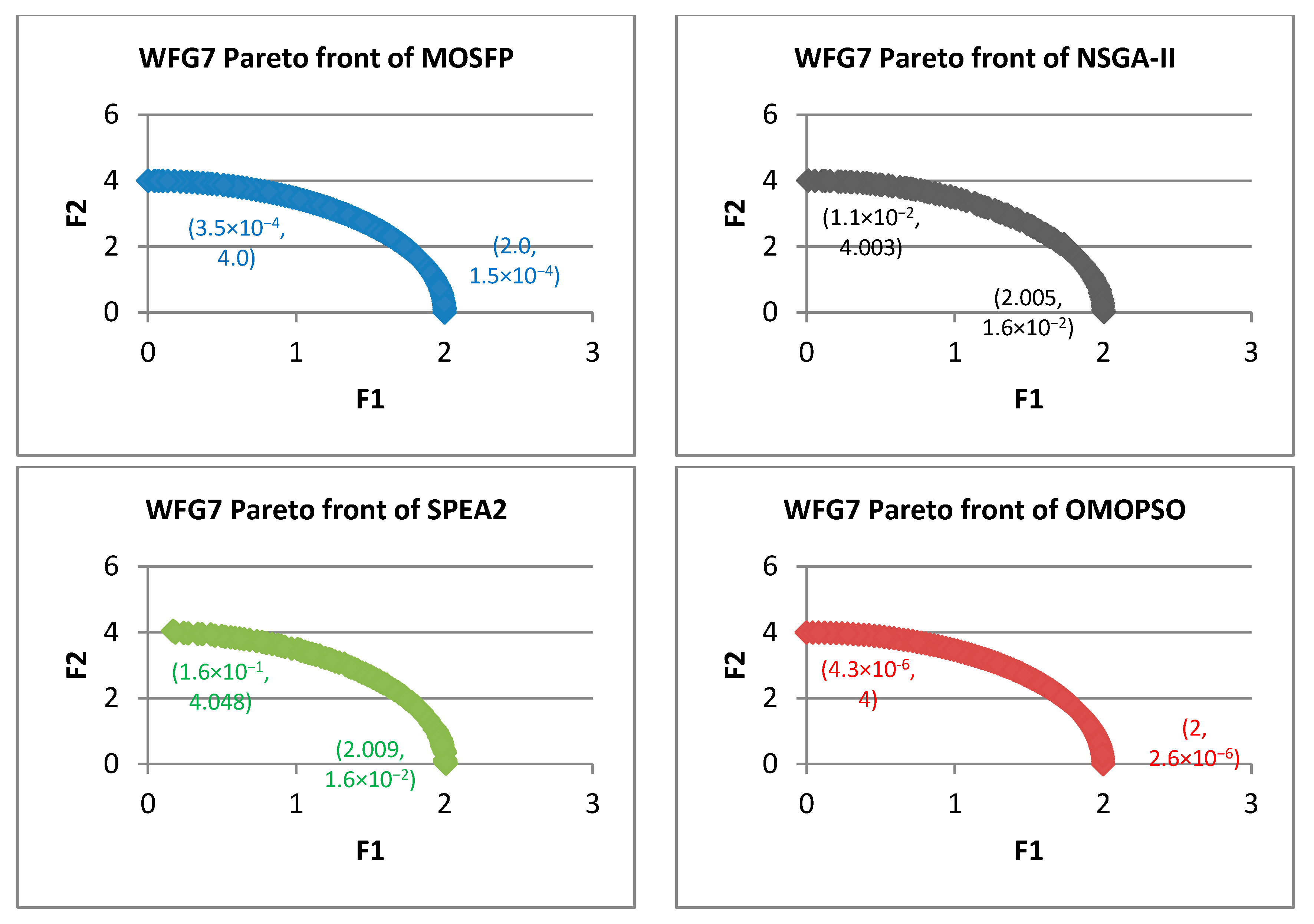
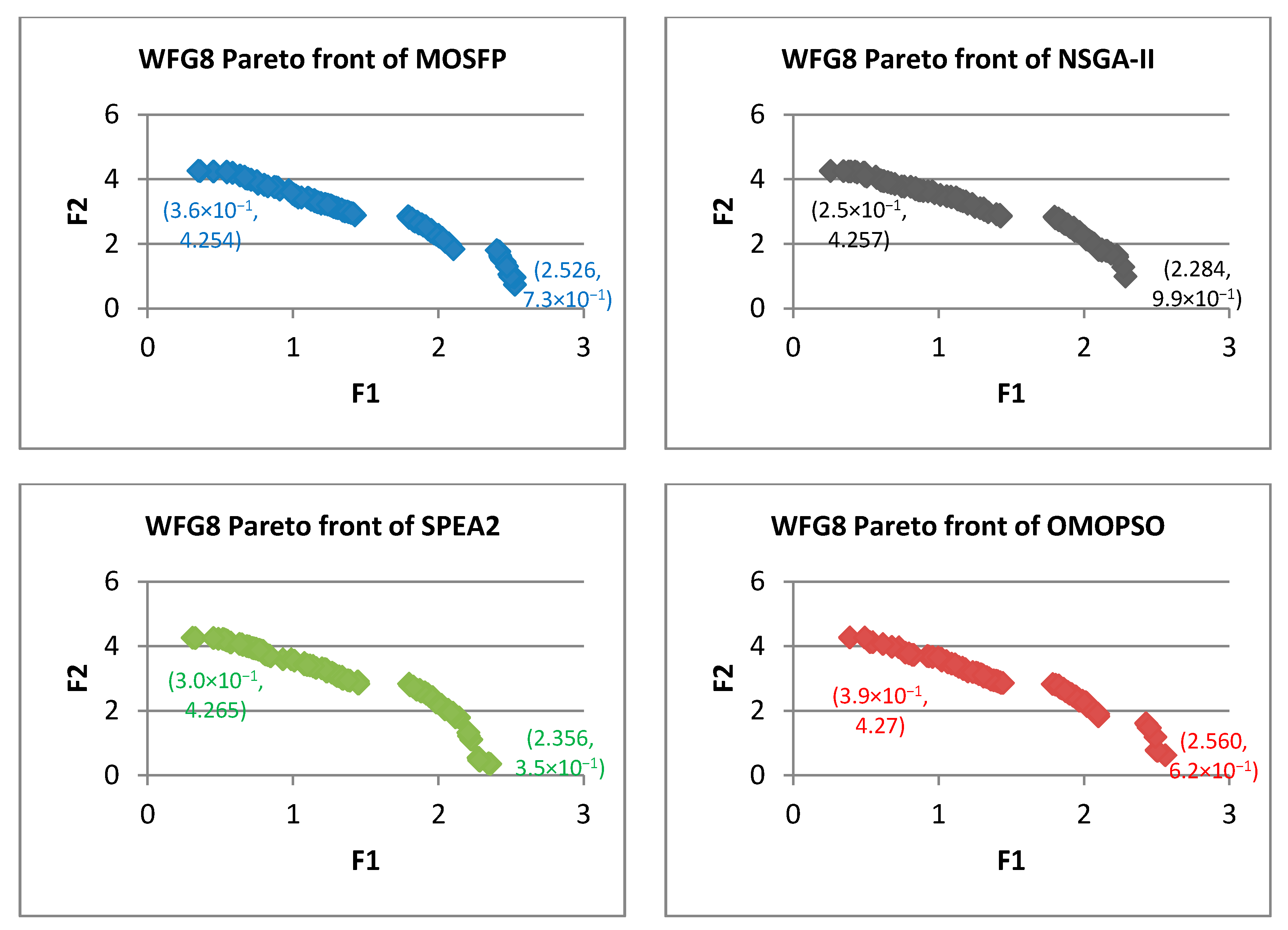
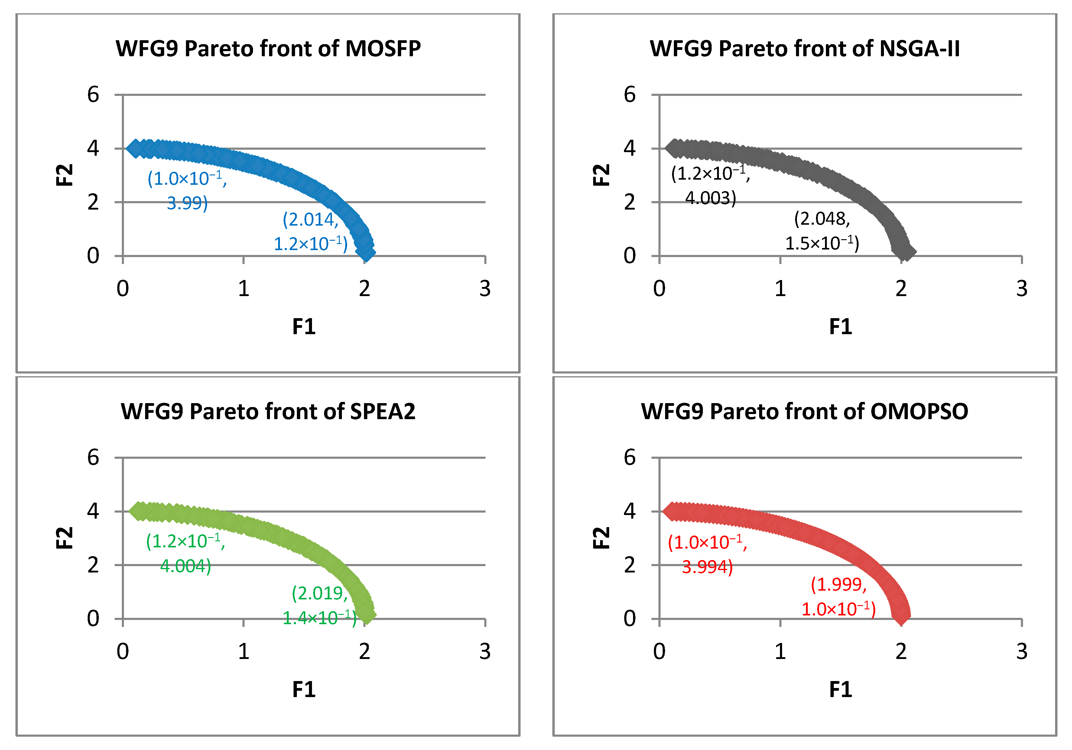
Table 5 summarized the best, worst, average, and median of , SP, and IGD measured from 5000 runs for WFG test functions. In this test, the OMOPSO algorithm has the best overall performance among all of the algorithms. However, the proposed MOSFP outperformed the OMOPSO, NSGA-II, and SPEA2 algorithms in solving WFG5 and WFG8 functions in terms of measurement and the best average of IGD for WFG5 function.
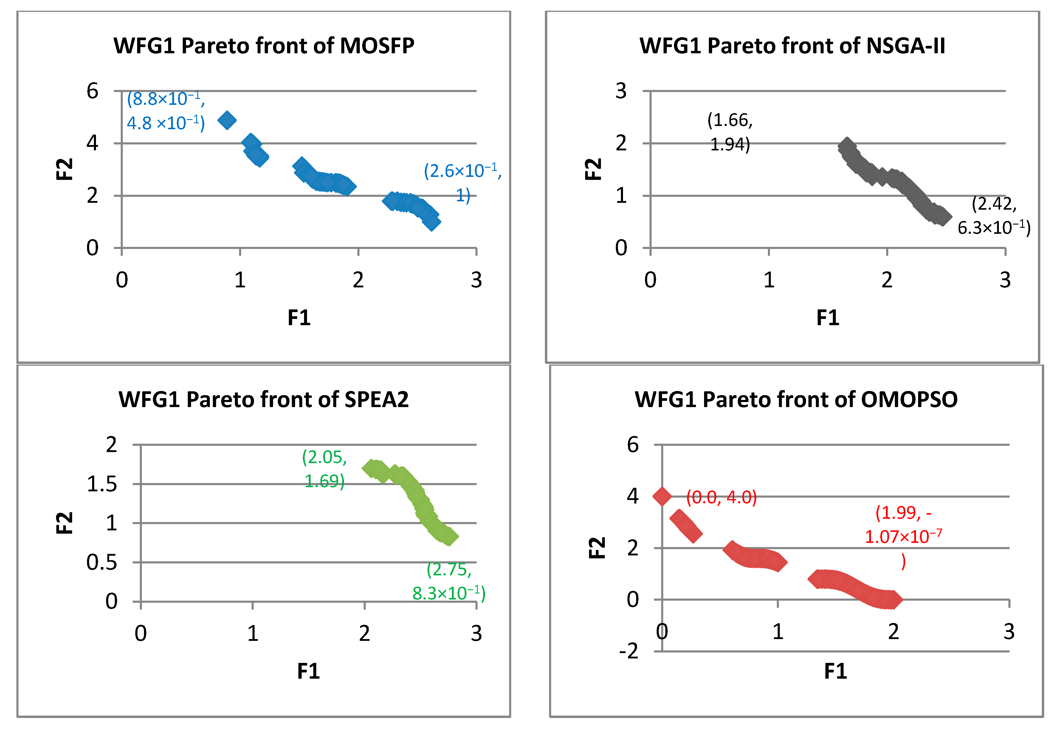
From Figure 7, Figure 8, Figure 9, Figure 10, Figure 11, Figure 12, Figure 13, Figure 14 and Figure 15, the proposed MOSFP demonstrates a high ability in obtaining the optimal extreme superior points of the true Pareto front i.e., (0, 4) and (2, 0) for WFG test functions. The proposed MOSFP obtained a close approximation of extreme superior points to the optimal point of the true Pareto front in solving WFG2, WFG3, WFG4, WFG5, WFG6, WFG7, and WFG9 test functions. For WFG8 function, all of the algorithms obtained inaccurate approximation of extreme superior points of true Pareto front. However, both the OMOPSO and MOSFP algorithms exhibit a better spread than NSGA-II and SPEA2 when their Pareto front is distributed into three parts when compared to NSGA-II and SPEA2 that are distributed into two parts. The same can also be observed in WFG1 test function when OMOPSO and MOSFP are more spread than NSGA-II and SPEA2.
6. Discussion
In this paper, MOSFP, OMOPSO, NSGA-II, and SPEA2 have been tested on ZDT and WFG benchmark functions. Three standard metrics are measured in the experiments, namely epsilon, spread, and inverted generational distance. For each algorithm tested in the experiment, the maximum generation for each function is set to 5000. The test is repeated 100 times for each objective to ensure the convergence of the results.
Overall, the proposed MOSFP algorithm outperformed both NSGA-II and SPEA2 algorithms in all of the benchmarks functions. Furthermore, MOSFP attained a high amount of points and a good approximation of the true Pareto front of all the benchmark functions. Additionally, MOSFP outperformed OMOPSO in solving the WFG5 problems, and obtained better solution sets than OMOPSO for true Pareto front of both ZDT3 and WFG8. The high-quality performance of the proposed MOSFP was reflected on the metrics of epsilon and IGD of WFG5, and epsilon of both ZDT3 and WFG8. This shows that the proposed MOSFP has a better convergence than the OMOPSO algorithm to explore the search space domain. Particularly, in solving the very complex disconnected functions, such as ZDT3 and benchmark suites that contain more than two objective functions, such as WFG5 and WFG8.
Based on that, MOSFP has the potential in solving the coverage problem of wireless sensor network (WSN), in which finding the optimal coverage required of finding the optimal distribution of sensor nodes on area estimated by kilometers or hectares [64]. Furthermore, MOSFP has the ability more than other algorithms in solving the problems with more than two objective functions, such as finding the optimal quality of services (QoS) of wireless, mobile and telecommunication networks [64,65,66], finding the optimal length and spacing of Yagi–Uda antenna design [12], engineering applications [63], finding the optimal products distribution through oil pipeline networks [19], and finding the optimal task allocation of stationary gas turbine [16].
7. Conclusions
The multi-objective optimization is used to manage the tradeoffs between a set of conflict objectives that consists of minimization problems and maximization problems. This management helps to find the optimal solution for these problems. Based on that, many single objective algorithms have been extended to deal with multi-objective problems. Examples of these algorithms are GA, which is extended to the NSGA-II and PSO algorithms, which is extended to different approaches such as OMOPSO.
SSO algorithm is a promising heuristic based algorithm that is inspired by sperm motility. This algorithm is suitable for solving different types of SOO, but requires an enhancement to work on MOOPs. In this paper, a MOO version of SSO algorithm has been developed using crowding, dominance archive, and mutation operations. We have proposed MOSFP, an extension of SSO for the multi-objective problem. The presented algorithm is easy to implement and improves the SSO capabilities of search space exploration by using a crowding and archive operators. Crowding operator is used to enhance the distribution and spreading of non-dominated solutions along the Pareto front, while the archive operator is used to fix the size of non-dominance solutions, which helps to increase the speed of the algorithm. The proposed algorithm is validated in two ways. First, we used the standard measurements and metrics that are currently adopted in the evolutionary MOO community. ZDT and WFG test suites have been chosen for this purpose. Three metrics, epsilon (), spread (SP), and inverted generational distance (IGD) have been chosen to compare between the proposed algorithm and other algorithms, such as OMOPSO, NSGA-II, and SPEA2. Second, the Pareto front of each algorithm for each objective function has been drawn, after that, compared based on the extreme superior points belonging to the true Pareto front. The results of these comparisons demonstrated that our method is a viable alternative since MOSFP has a higher ability to solve the problems of two objectives represented by ZDT test suites and problems of more than two objectives, represented by WFG test suites. Moreover, the average quality of MOSFP performance, spread and convergence are better than some of the best multi-objective optimization and evolutionary methods, known to date such as NSGA-II and SPEA2.
In the future, we will enhance the MOSFP by hybridizing it with other evolutionary or swarm intelligence algorithms to increase its efficiency and performance. Also, we will test it by solving different types of real world problems, such as the problems of wireless networks
Acknowledgments
The authors acknowledge University of Malaya for the financial support (University Malaya Research Grant (RP036(A,B,C)-15AET)) and facilitating in carrying out the work.
Author Contributions
The work was deduced from Hisham’s Ph.D. thesis as Mohd Yamani Idna Idris and Ismail Ahmedy supervised him along his study.
Conflicts of Interest
The authors declare no conflict of interest.
Appendix A
Part I: Zitzler-Deb-Thiele (ZDT) Test Suite
| No | Problem | Model | Domain |
| 1 | ZDT1 | ||
| 2 | ZDT2 | ||
| 3 | ZDT3 | ||
| 4 | ZDT6 |
Part II: Walking-Fish-Group (WFG) Test Suite
| No. | Problem | Type | Model |
| 5 | WFG1 | Shape | |
| t1 | |||
| t2 | |||
| t3 | |||
| t4 | |||
| 6 | WFG2 | Shape | |
| t1 | As t1 from WFG1. (linear shift) | ||
| t2 | |||
| t3 | |||
| 7 | WFG3 | Shape | |
| t1:3 | As t1:3 from WFG2. (linear shift, non-separable reduction, and weighted sum reduction.) | ||
| 8 | WFG4 | Shape | |
| t1 | |||
| t2 | |||
| 9 | WFG5 | Shape | |
| t1 | |||
| t2 | As t2 from WFG4 (Weighted sum reduction.) | ||
| 10 | WFG6 | Shape | |
| t1 | As t1 from WFG1. (Linear shift.) | ||
| t2 | |||
| 11 | WFG7 | Shape | |
| t1 | |||
| t2 | As t1 from WFG1. (Linear shift). | ||
| t3 | As t2 from WFG4. (weighted sum reduction.) | ||
| 12 | WFG8 | Shape | |
| t1 | |||
| t2 | As t1 from WFG1. (Linear shift). | ||
| t3 | As t2 from WFG4. (weighted sum reduction.) | ||
| 13 | WFG9 | Shape | |
| t1 | |||
| t2 | |||
| t3 | As t2 from WFG6. (non-separable reduction.) |
References
- Everson, R.M.; Fieldsend, J.E.; Singh, S. Full elite sets for multi-objective Optimization. In Proceedings of the 5th International Conference Adaptive Computing Design Manufacture (ACDM 2002), Devon, UK, 16–18 April 2002; pp. 343–354. [Google Scholar] [CrossRef]
- Knowles, J.D.; Corne, D.W. Approximating the nondominated front using the Pareto archived evolution strategy. Evolut. Comput. 2000, 8, 149–172. [Google Scholar] [CrossRef] [PubMed]
- Capitanescu, F.; Marvuglia, A.; Benetto, E.; Ahmadi, A.; Tiruta-Barna, L. Linear programming-based directed local search for expensive multi-objective optimization problems: Application to drinking water production plants. Eur. J. Oper. Res. 2017, 262, 322–334. [Google Scholar] [CrossRef]
- Sakawa, M. Fuzzy Sets and Interactive Multiobjective Optimization, 1st ed.; Singah, M.G., Ed.; Springer Science & Business Media: Higashi-Hiroshima, Japan, 2013; pp. 1–308. ISBN 978-1-4899-1633-4. [Google Scholar]
- Watanabe, K.; Hashem, M.M.A. Evolutionary Computations: New Algorithms and Their Applications to Evolutionary Robots, 1st ed.; Springer: Berlin/Heidelberg, Germany, 2004; Volume 147, pp. 1–172. ISBN 978-3-540-39883-7. [Google Scholar]
- Holland, J.H. Genetic algorithms. Sci. Am. 1992, 267, 66–73. [Google Scholar] [CrossRef]
- Kennedy, J.; Eberhart, R. Particle swarm optimization. In Proceedings of the IEEE International Conference on Neural Networks, Perth, Australia, 27 November–1 December 1995; pp. 1942–1948. [Google Scholar] [CrossRef]
- Coello, C.; Lamont, G.; Van-Veldhuizen, D. Evolutionary Algorithms for Solving Multiobjective Problems, 2nd ed.; Lamont-Veldhuizen, G.B., Ed.; Springer: New York, NY, USA, 2013; pp. 1–800. ISBN 978-0-387-36797-2. [Google Scholar]
- Srinivas, N.; Deb, K. Muiltiobjective optimization using nondominated sorting in genetic algorithms. Evolut. Comput. 1994, 2, 221–248. [Google Scholar] [CrossRef]
- Coello Coello, C.A. Mopso: A proposal for multiple objective particle swarm optimization. In Proceedings of the 2002 Congress on Evolutionary Computation (CEC 2002), Honolulu, HI, USA, 12–17 May 2002; pp. 1051–1056. [Google Scholar] [CrossRef]
- Sierra, M.R.; Coello, C.C. Improving pso-based multi-objective optimization using crowding, mutation and e-dominance, Evolutionary multi-criterion optimization. In Proceedings of the International Conference on Evolutionary Multi-Criterion Optimization, Guanajuato, Mexico, 9–11 March 2005; pp. 505–519. [Google Scholar] [CrossRef]
- Venkatarayalu, N.V.; Ray, T. Single and multi-objective design of yagi-uda antennas using computational intelligence, Evolutionary Computation. In Proceedings of the IEEE Evolutionary Computation (CEC’03), Canberra, ACT, Australia, 8–12 December 2003; pp. 1237–1242. [Google Scholar] [CrossRef]
- Watanabe, S.; Hiroyasu, T.; Miki, M. Parallel evolutionary multi-criterion optimization for mobile telecommunication networks optimization. Evolutionary Methods for Design, Optimization and Control with Applications to Industrial Problems. In Proceedings of the EUROGEN 2001, Athens, Greece, 19–21 September 2001; pp. 167–172. [Google Scholar]
- Shaw, K.; Nortcliffe, A.; Thompson, M.; Love, J.; Fleming, P.; Fonseca, C. Assessing the performance of multiobjective genetic algorithms for optimization of a batch process scheduling problem. In Proceedings of the IEEE 1999 Congress on Evolutionary Computation (CEC 99), Washington, DC, USA, 6–9 July 1999; pp. 37–45. [Google Scholar] [CrossRef]
- Barone, L.; While, L.; Hingston, P. Designing crushers with a multi-objective evolutionary algorithm. In Proceedings of the 4th Annual Conference on Genetic and Evolutionary Computation, New York, NY, USA, 9–13 July 2002; pp. 995–1002. [Google Scholar] [CrossRef]
- Buche, D.; Stoll, P.; Dornberger, R.; Koumoutsakos, P. Multiobjective evolutionary algorithm for the optimization of noisy combustion processes. IEEE Trans. Syst. Man Cybern. Part C Appl. Rev. 2002, 32, 460–473. [Google Scholar] [CrossRef]
- Engrand, P. A multi-Objective Optimization Approach Based on Simulated Annealing and Its Application to Nuclear Fuel Management. Electricite de France 1998, 30, 1–8. [Google Scholar]
- Hughes, E.J. Swarm guidance using a multi-objective co-evolutionary on-line evolutionary algorithm. In Proceedings of the IEEE Congress on Evolutionary Computation (CEC2004), Portland, OR, USA, 19–23 June 2004; pp. 2357–2363. [Google Scholar] [CrossRef]
- Garcia, J.; Martin, J.R.; Gonzales, A.; Blanco, P. Hybrid heuristic and mathematical programming in oil pipelines networks. In Proceedings of the IEEE Congress on Evolutionary Computation (CEC2004), Portland, OR, USA, 19–23 June 2004; pp. 1479–1486. [Google Scholar] [CrossRef]
- Zitzler, E.; Laumanns, M.; Bleuler, S. A tutorial on evolutionary multiobjective optimization. In Metaheuristics for Multiobjective Optimization, 1st ed.; Gandibleux, X., Sevaux, M., Sörensen, K., T’kindt, V., Eds.; Springer: Berlin/Heidelberg, Germany, 2004; Volume 535, pp. 3–37. ISBN 978-3-540-20637-8. [Google Scholar]
- Shehadeh, H.A.; Idris, M.Y.I.; Ahmedy, I.; Noor, N.M. Sperm Swarm Optimization (SSO) Algorithm. Comput. Intell. Neurosci. 2017. under review. [Google Scholar]
- Tung, C.K.; Fiore, A.G.; Ardon, F.; Suarez, S.S.; Wu, M. Collective dynamics of sperm in viscoelastic fluid. APS Meet. Abstr. 2016, 2, 10–30. [Google Scholar]
- Nalepa, J.; Kawulok, M. A memetic algorithm to select training data for support vector machines. In Proceedings of the 2014 Annual Conference on Genetic and Evolutionary Computation ACM, Vancouver, BC, Canada, 12–16 July 2014; pp. 573–580. [Google Scholar] [CrossRef]
- Das Neves, J.; Bahia, M.F. Gels as vaginal drug delivery systems. Int. J. Pharm. 2006, 318, 1–14. [Google Scholar] [CrossRef] [PubMed]
- Rodrigues, J.; Caldeira, J.; Vaidya, B. A novel intra-body sensor for vaginal temperature monitoring. Sensor 2009, 9, 2797–2808. [Google Scholar] [CrossRef] [PubMed]
- Borges, S.F.; Silva, J.G.; Teixeira, P.C. Survival and biofilm formation of Listeria monocytogenes in simulated vaginal fluid: Influence of pH and strain origin. FEMS Immunol. Med. Microbiol. 2011, 62, 315–320. [Google Scholar] [CrossRef] [PubMed]
- Edmunds, M.W.; Mayhew, M.S. Pharmacology for the Primary Care Provider-E-Book, 1st ed.; Elsevier Health Sciences: Washington, DC, USA, 2013; pp. 1–863. ISBN 978-0-323-08790-2. [Google Scholar]
- Bahat, A.; Caplan, S.R.; Eisenbach, M. Thermotaxis of human sperm cells in extraordinarily shallow temperature gradients over a wide range. PLoS ONE 2012, 7, e41915. [Google Scholar] [CrossRef] [PubMed]
- Christian Nicole. 2013. Available online: https://christiannicole72838.wordpress.com/2013/06/26/from-the-figure-for-women-to-understand-their-own-sexual-organs-gender/ (accessed on 21 September 2017).
- Health. 2011. Available online: http://health-of-people.blogspot.com/2011/03/interestingly-statistics-of-physical.html (accessed on 28 July 2017).
- Bahat, A.; Eisenbach, M. Sperm thermotaxis. Mol. Cell. Endocrinol. 2006, 252, 115–119. [Google Scholar] [CrossRef] [PubMed]
- Engelbrecht, A.P. Fundamentals of Computational Swarm Intelligence; John Wiley & Sons: Hoboken, NJ, USA, 2006; pp. 1–672. ISBN 0470091916. [Google Scholar]
- Chamaani, S.; Mirtaheri, S.A.; Teshnehlab, M.; Shooredeli, M.A. Modified multi-objective particle swarm optimization for electromagnetic absorber design. In Proceedings of the IEEE Asia-Pacific Conference on Applied Electromagnetics APACE, Kuala Lampur, Malaysia, 4–6 December 2007; pp. 1–5. [Google Scholar] [CrossRef]
- Lindroth, P.; Patriksson, M.; Strömberg, A.B. Approximating the Pareto optimal set using a reduced set of objective functions. Eur. J. Oper. Res. 2010, 207, 1519–1534. [Google Scholar] [CrossRef]
- Zheng, X.; Liu, H. A scalable coevolutionary multi-objective particle swarm optimizer. Int. J. Comput. Intell. Syst. 2010, 3, 590–600. [Google Scholar] [CrossRef]
- Lei, J.; Fu, G.; Yang, L.; Fu, D. Multi-objective optimization design of the yagi-uda antenna with an x-shape driven dipole. J. Electromagn. Waves Appl. 2007, 21, 963–972. [Google Scholar] [CrossRef]
- Lee, Y.H.; Cahill, B.J.; Porter, S.J.; Marvin, A.C. A novel evolutionary learning technique for multi-objective array antenna optimization. Prog. Electromagn. Res. 2004, 48, 125–144. [Google Scholar] [CrossRef]
- Coello, C.A.C.; Pulido, G.T.; Lechuga, M.S. Handling multiple objectives with particle swarm optimization. IEEE Trans. Evolut. Comput. 2004, 8, 256–279. [Google Scholar] [CrossRef]
- Deb, K.; Pratap, A.; Agarwal, S.; Meyarivan, T. A fast and elitist multiobjective genetic algorithm: Nsga-ii. IEEE Trans. Evolut. Comput. 2002, 6, 182–197. [Google Scholar] [CrossRef]
- Ray, T.; Liew, K. A swarm metaphor for multiobjective design optimization. Eng. Optim. 2002, 34, 141–153. [Google Scholar] [CrossRef]
- Li, X. A non-dominated sorting particle swarm optimizer for multiobjective optimization. In Proceedings of the Genetic and Evolutionary Computation—GECCO 2003, Chicago, IL, USA, 3 August 2003; Springer: Berlin, Germany, 2003; p. 198. [Google Scholar] [CrossRef]
- Laumanns, M.; Thiele, L.; Deb, K.; Zitzler, E. Combining convergence and diversity in evolutionary multiobjective optimization. Evolut. Comput. 2002, 10, 263–282. [Google Scholar] [CrossRef] [PubMed]
- Yue, X.; Guo, Z.; Yin, Y.; Liu, X. Many-objective E-dominance dynamical evolutionary algorithm based on adaptive grid. Soft Comput. 2016, 2, 1–10. [Google Scholar] [CrossRef]
- Guzek, M.; Diaz, C.O.; Pecero, J.E.; Bouvry, P.; Zomaya, A.Y. Impact of voltage levels number for energy-aware bi-objective dag scheduling for multi-processors systems. In Proceedings of the International Conference on Advances in Information Technology, Bangkok, Thailand, 6–7 December 2012; pp. 70–80. [Google Scholar] [CrossRef]
- Guzek, M.; Pecero, J.E.; Dorronsoro, B.; Bouvry, P. Multi-objective evolutionary algorithms for energy-aware scheduling on distributed computing systems. Appl. Soft Comput. 2014, 24, 432–446. [Google Scholar] [CrossRef]
- Dai, C.; Wang, Y.; Hu, L. An improved α-dominance strategy for many-objective optimization problems. Soft Comput. 2016, 20, 1105–1111. [Google Scholar] [CrossRef]
- Bezerra, L.C.; López-Ibáñez, M.; Stützle, T. An empirical assessment of the properties of inverted generational distance on multi-and many-objective optimization. In Proceedings of the International Conference on Evolutionary Multi-Criterion Optimization, Münster, Germany, 19–22 March 2017; pp. 31–45. [Google Scholar] [CrossRef]
- Yang, S.; Ong, Y.S.; Jin, Y. (Eds.) Evolutionary Computation in Dynamic and Uncertain Environments, 1st ed.; Springer: Berlin/Heidelberg, Germany, 2007; Volume 51, pp. 1–605. ISBN 3-540-49772-2. [Google Scholar]
- Monroy, R.; Arroyo-Figueroa, G.; Sucar, L.E.; Sossa, H. Micai Advances in artificial intelligence. In Proceedings of the Third Mexican International Conference on Artificial Intelligence, Mexico City, Mexico, 26–30 April 2004; pp. 622–631. [Google Scholar] [CrossRef]
- Jiang, S.; Cai, Z. A novel hybrid particle swarm optimization for multi-objective problems. In Proceedings of the International Conference on Artificial Intelligence and Computational Intelligence, Shanghai, China, 7–8 November 2009; pp. 28–37. [Google Scholar] [CrossRef]
- Jiang, S.; Ong, Y.S.; Zhang, J.; Feng, L. Consistencies and contradictions of performance metrics in multiobjective optimization. IEEE Trans. Cybern. 2014, 44, 2391–2404. [Google Scholar] [CrossRef] [PubMed]
- Riquelme, N.; Von Lücken, C.; Baran, B. Performance metrics in multi-objective optimization, Computing. In Proceedings of the IEEE Conference of Latin American (CLEI), Arequipa, Peru, 19–23 October 2015; pp. 1–11. [Google Scholar] [CrossRef]
- Hamdy, M.; Nguyen, A.-T.; Hensen, J.L. A performance comparison of multi-objective optimization algorithms for solving nearly-zero-energy-building design problems. Energy Build. 2016, 121, 57–71. [Google Scholar] [CrossRef]
- Acampora, G.; Ishibuchi, H.; Vitiello, A. A comparison of multi-objective evolutionary algorithms for the ontology meta-matching problem. In Proceedings of the IEEE Congress on Evolutionary Computation (CEC), Beijing, China, 6–11 July 2014; pp. 413–420. [Google Scholar] [CrossRef]
- Gharari, R.; Poursalehi, N.; Abbasi, M.; Aghaie, M. Implementation of strength pareto evolutionary algorithm ii in the multiobjective burnable poison placement optimization of kwu pressurized water reactor. Nucl. Eng. Technol. 2016, 48, 1126–1139. [Google Scholar] [CrossRef]
- Eckart, Z.; Marco, L.; Lothar, T. SPEA2: Improving the strength pareto evolutionary algorithm for multiobjective optimization. In Proceedings of the EUROGEN’2001 Eurogen, Evolutionary Method for Design: Optimization and Control for Industrial Problem, Barcelona, Spain, 19–21 September 2001; pp. 1–21. [Google Scholar] [CrossRef]
- Theophila, B. Study of Hardware and Software Optimizations of Spea2 on Hybrid Fpgas, 1st ed.; Lukowiak, M., Amuso, V.J., Shaaban, R., Jason, E., Eds.; Rochester Institute of Technology: Rochester, NY, USA, 2008; pp. 1–79. [Google Scholar]
- Bandyopadhyay, S.; Bhattacharya, R. On some aspects of nature-based algorithms to solve multi-objective problems. In Artificial intelligence, Evolutionary Computing and Metaheuristics; Yang, X., Ed.; Springer: Berlin/Heidelberg, Germany, 2013; Chapter 9; pp. 477–524. ISBN 978-3-642-29693-2. [Google Scholar]
- Pollack, S.L.; Hicks, H.T.; Harrison, W.J. Decision Tables Theory and Practice; Cannian, R.G., Cougar, J., Eds.; John Wiley & Sons: Hoboken, NJ, USA, 1971; pp. 1–179. ISBN 047169150X. [Google Scholar]
- Huband, S.; Hingston, P.; Barone, L.; While, L. A review of multiobjective test problems and a scalable test problem toolkit. IEEE Trans. Evolut. Comput. 2006, 10, 477–506. [Google Scholar] [CrossRef]
- Huband, S.; Barone, L.; While, R.L.; Hingston, P. A scalable multi-objective test problem toolkit. In Proceedings of the International Conference on Evolutionary Multi-Criterion Optimization, Guanajuato, Mexico, 9–11 March 2005; pp. 280–295. [Google Scholar] [CrossRef]
- Deb, K.; Thiele, L.; Laumanns, M.; Zitzler, E. Scalable multi-objective optimization test problems. In Proceedings of the IEEE Congress on Evolutionary Computation (CEC’2002), Honolulu, HI, USA, 12–17 May 2002; pp. 825–830. [Google Scholar] [CrossRef]
- Chase, N.; Rademacher, M.; Goodman, E.; Averill, R.; Sidhu, R. A benchmark study of multi-objective optimization methods. Red Cedar Technol. 2009, 6, 1–24. [Google Scholar]
- Bara’a, A.A.; Khalil, E.A.; Cosar, A. Multi-objective evolutionary routing protocol for efficient coverage in mobile sensor networks. Soft Comput. 2015, 19, 2983–2995. [Google Scholar] [CrossRef]
- Ibdah, Y.; Ding, Y. Path loss models for low-height mobiles in forest and urban. Wirel. Person. Commun. 2017, 92, 455–465. [Google Scholar] [CrossRef]
- Hamdan, M.; Yassein, M.B.; Shehadeh, H.A. Multi-objective optimization modeling of interference in home health care sensors. In Proceedings of the IEEE 11th International Conference on Innovations in Information Technology (IIT), Dubai, UAE, 1–3 November 2015; pp. 219–224. [Google Scholar] [CrossRef]
Figure 1.
The winner and other sperms reach the egg [21].
Figure 1.
The winner and other sperms reach the egg [21].

Figure 2.
Diversity metrics illustration of two components (spread and distribution) [37]: (a) good distribution, but poor spread; (b) poor distribution, but good spread.
Figure 2.
Diversity metrics illustration of two components (spread and distribution) [37]: (a) good distribution, but poor spread; (b) poor distribution, but good spread.

Figure 3.
Pareto fronts obtained by all the algorithms for ZDT1.

Figure 4.
Pareto fronts obtained by all the algorithms for ZDT2.
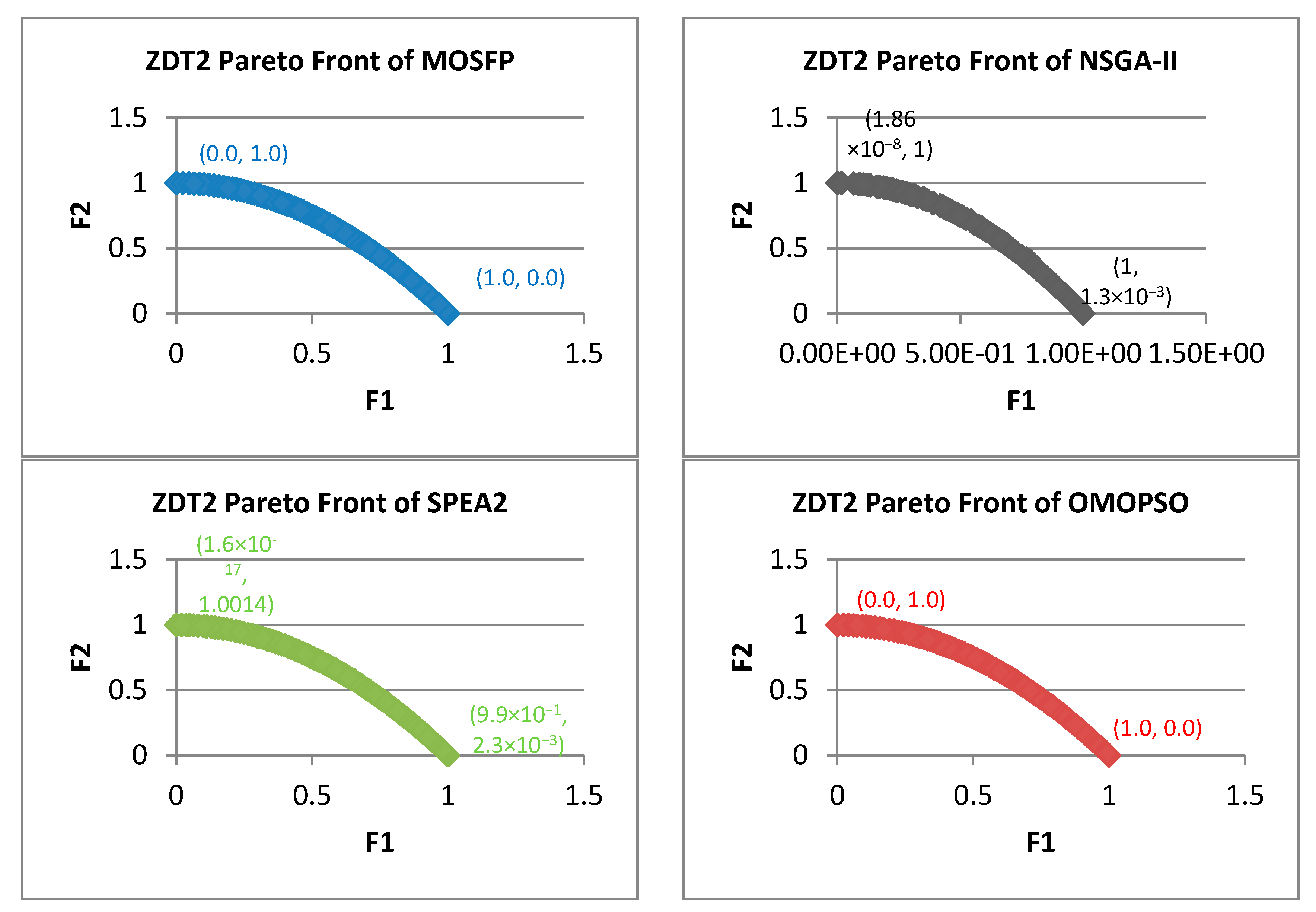
Figure 5.
Pareto fronts obtained by all the algorithms for ZDT3.
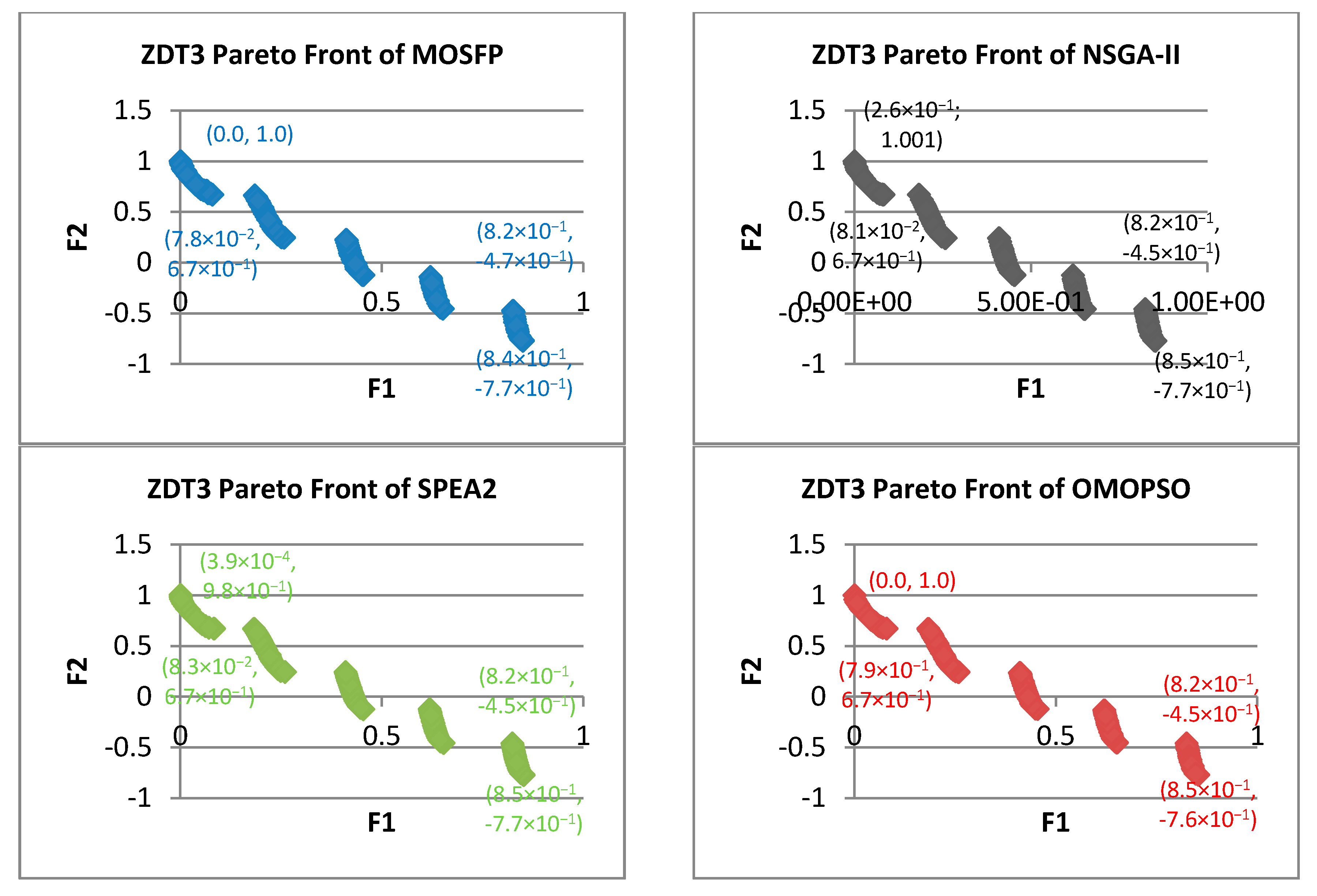
Figure 6.
Pareto fronts obtained by all the algorithms for ZDT6.

Figure 7.
Pareto fronts obtained by all the algorithms for WFG1.

Figure 8.
Pareto fronts obtained by all the algorithms for WFG2.
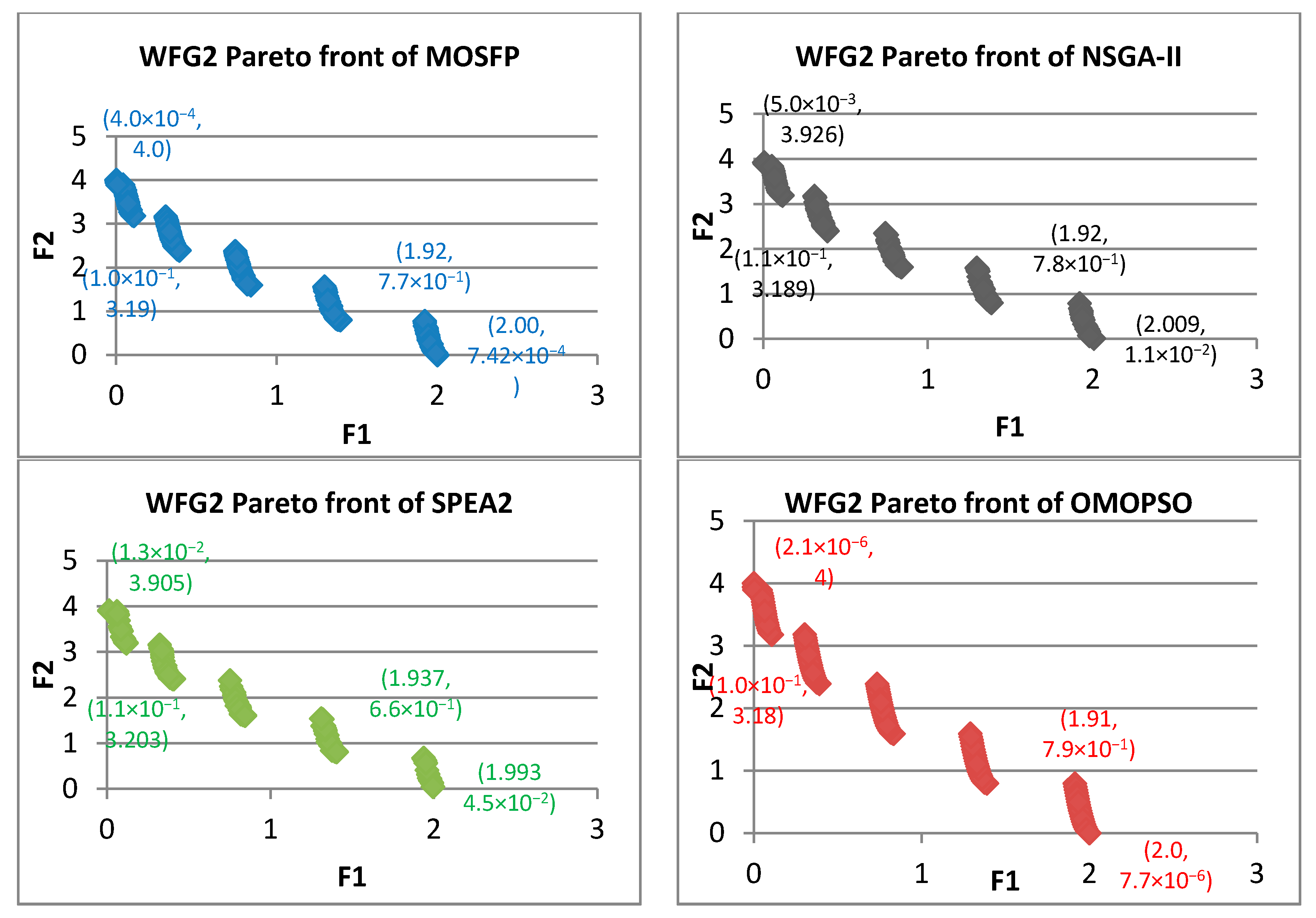
Figure 9.
Pareto fronts obtained by all the algorithms for WFG3.

Figure 10.
Pareto fronts obtained by all the algorithms for WFG4.

Figure 11.
Pareto fronts obtained by all the algorithms for WFG5.

Figure 12.
Pareto fronts obtained by all the algorithms for WFG6.

Figure 13.
Pareto fronts obtained by all the algorithms for WFG7.

Figure 14.
Pareto fronts obtained by all the algorithms for WFG8.

Figure 15.
Pareto fronts obtained by all the algorithms for WFG9.


Table 1.
Analysis of ZDT benchmark functions [60].
Table 1.
Analysis of ZDT benchmark functions [60].
| Name | ZDT1 | ZDT2 | ZDT3 | ZDT6 | ||||
|---|---|---|---|---|---|---|---|---|
| Objective | f1 | f2 | f1 | f2 | f1 | f2 | f1 | f2 |
| R3: # Parameters | 1 | ✓ | 1 | ✓ | 1 | ✓ | 1 | ✓ |
| F2: Separability | S | S | S | S | S | S | S | S |
| F5: Modality | U | U | U | U | U | M | U | U |
| R1: No Extremal | ✗ | ✗ | ✗ | ✗ | ||||
| R2: No Medial | ✓ | ✓ | ✓ | ✓ | ||||
| R5: Diss. Domains | ✗ | ✗ | ✗ | ✗ | ||||
| R6: Diss. Ranges | ✗ | ✗ | ✓ | ✓ | ||||
| R7: Optima known | ✓ | ✓ | ✓ | ✓ | ||||
| F1: Geometry | convex | concave | disconnected | concave | ||||
| F3: Bias | - | - | - | + | ||||
| F4a: Pareto Many-to-one | - | - | - | + | ||||
| F4b: Flat Regions | - | - | - | - | ||||
Table 2.
Analysis of WFG benchmark functions [60].
Table 2.
Analysis of WFG benchmark functions [60].
| Name | Objective | F2: Separability | Modality | Bias | Geometry |
|---|---|---|---|---|---|
| WFG1 | f1:M | S | U | Polynomial, flat | Convex, Mixed |
| WFG2 | f1:M-1 fM | NS | U | − | Convex, disconnected |
| NS | M | ||||
| WFG3 | f1:M | NS | U | − | Linear, degenerate |
| WFG4 | f1:M | S | M | − | Concave |
| WFG5 | f1:M | S | D | − | Concave |
| WFG6 | f1:M | NS | U | − | Concave |
| WFG7 | f1:M | S | U | Parameter dependent | Concave |
| WFG8 | f1:M | NS | U | Parameter dependent | Concave |
| WFG9 | f1:M | NS | M, D | Parameter dependent | Concave |
Table 3.
Parameters of the algorithms.
| Parameters | MOSFP | OMOPSO | NSGA-II | SPEA2 |
|---|---|---|---|---|
| Population size | 100 | 100 | 100 | 100 |
| Archive size | (winner) 100 | 100 | (Elite) 100 | 100 |
| Mating pool size | - | - | - | 100 |
| Maximum generation | 5000 | 5000 | 5000 | 5000 |
| Crossover probability | - | - | 0.9 | 0.9 |
| Mutation probability | 1/d where d is the variable code size | |||
Table 4.
Comparison of experimental results between multi-objective optimization algorithm based on sperm fertilization procedure (MOSFP), optimized multi-objective particle swarm optimization (OMOPSO), non-dominated sorting genetic algorithm II (NSGA-II), and strength Pareto evolutionary algorithm 2 (SPEA2) in terms of epsilon () spread (SP), and inverted generational distance (IGD) for Zitzler-Deb-Thiele (ZDT) test functions.
| Method | Metrics | |||||||||||
|---|---|---|---|---|---|---|---|---|---|---|---|---|
| SP | IGD | |||||||||||
| Best | Worst | Aver. | Med. | Best | Worst | Aver. | Med. | Best | Worst | Aver. | Med. | |
| ZDT1 | ||||||||||||
| MOSFP | 5.01 × 10⁻³ | 5.57 × 10⁻³ | 5.27 × 10⁻³ | 5.25 × 10⁻³ | 2.76 × 10⁻² | 9.85 × 10⁻² | 6.23 × 10⁻² | 6.22 × 10⁻² | 3.44 × 10⁻⁵ | 3.61 × 10⁻⁵ | 3.51 × 10⁻⁵ | 3.51 × 10⁻⁵ |
| OMOPSO | 4.92 × 10⁻³ | 5.40 × 10⁻³ | 5.15 × 10⁻³ | 5.15 × 10⁻³ | 3.29 × 10⁻² | 8.74 × 10⁻² | 5.54 × 10⁻² | 5.52 × 10⁻² | 3.39 × 10⁻⁵ | 3.60 × 10⁻⁵ | 3.48 × 10⁻⁵ | 3.48 × 10⁻⁵ |
| NSGA-II | 1.11 × 10⁻¹ | 2.67 × 10⁻¹ | 1.61 × 10⁻¹ | 1.51 × 10⁻¹ | 5.84 × 10⁻¹ | 8.17 × 10⁻¹ | 6.80 × 10⁻¹ | 6.87 × 10⁻¹ | 7.65 × 10⁻⁴ | 1.92 × 10⁻³ | 1.18 × 10⁻³ | 1.14 × 10⁻³ |
| SPEA2 | 1.60 × 10⁻¹ | 4.58 × 10⁻¹ | 2.82 × 10⁻¹ | 2.74 × 10⁻¹ | 8.92 × 10⁻¹ | 6.11 × 10⁻¹ | 7.43 × 10⁻¹ | 7.35 × 10⁻¹ | 1.04 × 10⁻³ | 2.71 × 10⁻³ | 1.76 × 10⁻³ | 1.72 × 10⁻³ |
| ZDT2 | ||||||||||||
| MOSFP | 5.018 × 10⁻³ | 5.65 × 10⁻³ | 5.27 × 10⁻³ | 5.28 × 10⁻³ | 2.75 × 10⁻² | 9.95 × 10⁻² | 5.62 × 10⁻² | 5.41 × 10⁻² | 3.41 × 10⁻⁵ | 3.60 × 10⁻⁵ | 3.49 × 10⁻⁵ | 3.49 × 10⁻⁵ |
| OMOPSO | 4.93 × 10⁻³ | 5.32 × 10⁻³ | 5.13 × 10⁻³ | 5.14 × 10⁻³ | 2.45 × 10⁻² | 8.30 × 10⁻² | 5.53 × 10⁻² | 5.56 × 10⁻² | 3.43 × 10⁻⁵ | 3.56 × 10⁻⁵ | 3.48 × 10⁻⁵ | 3.47 × 10⁻⁵ |
| NSGA-II | 3.46 × 10⁻¹ | 1.457 | 6.32 × 10⁻¹ | 5.88 × 10⁻¹ | 6.38 × 10⁻¹ | 1.011 | 8.33 × 10⁻¹ | 8.32 × 10⁻¹ | 1.54 × 10⁻³ | 9.44 × 10⁻³ | 3.10 × 10⁻³ | 2.75 × 10⁻³ |
| SPEA2 | 5.21 × 10⁻¹ | 1.775 | 1.107 | 1.051 | 8.14 × 10⁻¹ | 1.0162 | 9.38 × 10⁻¹ | 9.51 × 10⁻¹ | 2.50 × 10⁻³ | 1.16 × 10⁻² | 6.34 × 10⁻³ | 5.31 × 10⁻³ |
| ZDT3 | ||||||||||||
| MOSFP | 3.37 × 10⁻³ | 5.28 × 10⁻³ | 4.13 × 10⁻³ | 4.11 × 10⁻³ | 6.99 × 10⁻¹ | 7.02 × 10⁻¹ | 7.01 × 10⁻¹ | 7.01 × 10⁻¹ | 2.78 × 10⁻⁵ | 3.08 × 10⁻⁵ | 2.91 × 10⁻⁵ | 2.91 × 10⁻⁵ |
| OMOPSO | 3.54 × 10⁻³ | 5.25 × 10⁻³ | 4.18 × 10⁻³ | 4.06 × 10⁻³ | 6.99 × 10⁻¹ | 7.01 × 10⁻¹ | 7.00 × 10⁻¹ | 7.00 × 10⁻¹ | 2.74 × 10⁻⁵ | 3.04 × 10⁻⁵ | 2.86 × 10⁻⁵ | 2.86 × 10⁻⁵ |
| NSGA-II | 1.51 × 10⁻¹ | 3.36 × 10⁻¹ | 2.10 × 10⁻¹ | 2.01 × 10⁻¹ | 7.82 × 10⁻¹ | 9.39 × 10⁻¹ | 8.63 × 10⁻¹ | 8.62 × 10⁻¹ | 3.96 × 10⁻⁴ | 1.40 × 10⁻³ | 8.73 × 10⁻⁴ | 8.87 × 10⁻⁴ |
| SPEA2 | 1.91 × 10⁻¹ | 6.06 × 10⁻¹ | 2.92 × 10⁻¹ | 2.86 × 10⁻¹ | 7.88 × 10⁻¹ | 9.37 × 10⁻¹ | 8.64 × 10⁻¹ | 8.62 × 10⁻¹ | 7.43 × 10⁻⁴ | 1.98 × 10⁻³ | 1.30 × 10⁻³ | 1.31 × 10⁻³ |
| ZDT6 | ||||||||||||
| MOSFP | 5.32 × 10⁻³ | 6.53 × 10⁻³ | 5.90 × 10⁻³ | 5.91 × 10⁻³ | 1.33 × 10⁻¹ | 1.81 × 10⁻¹ | 1.55 × 10⁻¹ | 1.55 × 10⁻¹ | 3.21 × 10⁻⁵ | 3.35 × 10⁻⁵ | 3.27 × 10⁻⁵ | 3.27 × 10⁻⁵ |
| OMOPSO | 4.73 × 10⁻³ | 9.00 × 10⁻³ | 5.59 × 10⁻³ | 5.42 × 10⁻³ | 5.59 × 10⁻² | 2.53 × 10⁻¹ | 1.13 × 10⁻¹ | 1.08 × 10⁻¹ | 3.09 × 10⁻⁵ | 3.41 × 10⁻⁵ | 3.19 × 10⁻⁵ | 3.17 × 10⁻⁵ |
| NSGA-II | 2.34 × 10⁻² | 3.53 × 10⁻² | 2.71 × 10⁻² | 2.65 × 10⁻² | 6.04 × 10⁻² | 1.36 | 7.41 × 10⁻¹ | 9.53 × 10⁻¹ | 4.67 × 10⁻⁵ | 1.37 × 10⁻³ | 2.03 × 10⁻⁴ | 1.60 × 10⁻⁴ |
| SPEA2 | 1.85 × 10⁻² | 3.84 × 10⁻¹ | 6.98 × 10⁻² | 6.09 × 10⁻² | 9.03 × 10⁻¹ | 1.436 | 1.332 | 1.345 | 1.99 × 10⁻⁴ | 2.29 × 10⁻⁴ | 2.04 × 10⁻⁴ | 2.03 × 10⁻⁴ |
Table 5.
Comparison of experimental results between MOSFP, OMOPSO, NSGA-II, and SPEA2 in terms of epsilon ( ) spread (SP), and inverted generational distance (IGD) for WFG test functions.
Table 5.
Comparison of experimental results between MOSFP, OMOPSO, NSGA-II, and SPEA2 in terms of epsilon ( ) spread (SP), and inverted generational distance (IGD) for WFG test functions.
| Method | Metrics | |||||||||||
|---|---|---|---|---|---|---|---|---|---|---|---|---|
| SP | IGD | |||||||||||
| Best | Worst | Aver. | Med. | Best | Worst | Aver. | Med. | Best | Worst | Aver. | Med. | |
| WFG1 | ||||||||||||
| MOSFP | 8.59× 10⁻¹ | 1.199 | 1.092 | 1.094 | 8.01 × 10⁻¹ | 1.057 | 9.31 × 10⁻¹ | 9.31 × 10⁻¹ | 2.72 × 10⁻³ | 4.93 × 10⁻³ | 4.33 × 10⁻³ | 4.37 × 10⁻³ |
| OMOPSO | 7.68 × 10⁻² | 1.022 | 1.61 × 10⁻¹ | 1.45 × 10⁻¹ | 7.41 × 10⁻¹ | 1.238 | 8.42 × 10⁻¹ | 8.33 × 10⁻¹ | 3.04 × 10⁻⁵ | 3.49 × 10⁻³ | 1.05 × 10⁻⁴ | 4.81 × 10⁻⁵ |
| NSGA-II | 1.441 | 2.020 | 1.740 | 1.746 | 8.63 × 10⁻¹ | 1.030 | 9.37 × 10⁻¹ | 9.33 × 10⁻¹ | 3.93 × 10⁻³ | 6.17 × 10⁻³ | 5.06 × 10⁻³ | 5.07 × 10⁻³ |
| SPEA2 | 1.562 | 2.227 | 1.923 | 1.922 | 8.08 × 10⁻¹ | 1.266 | 1.080 | 1.070 | 4.46 × 10⁻³ | 7.02 × 10⁻³ | 5.77 × 10⁻³ | 5.73 × 10⁻³ |
| WFG2 | ||||||||||||
| MOSFP | 1.14 × 10⁻² | 1.92 × 10⁻² | 1.42 × 10⁻² | 1.39 × 10⁻² | 7.57 × 10⁻¹ | 7.96 × 10⁻¹ | 7.77 × 10⁻¹ | 7.74 × 10⁻¹ | 5.07 × 10⁻⁵ | 7.37 × 10⁻⁵ | 5.91 × 10⁻⁵ | 5.90 × 10⁻⁵ |
| OMOPSO | 7.48 × 10⁻³ | 1.04 × 10⁻² | 9.01 × 10⁻³ | 8.94 × 10⁻³ | 7.56 × 10⁻¹ | 7.59 × 10⁻¹ | 7.57 × 10⁻¹ | 7.57 × 10⁻¹ | 3.81 × 10⁻⁵ | 4.22 × 10⁻⁵ | 4.01 × 10⁻⁵ | 4.00 × 10⁻⁵ |
| NSGA-II | 1.59 × 10⁻² | 8.15 × 10⁻¹ | 4.83 × 10⁻¹ | 7.99 × 10⁻¹ | 7.86 × 10⁻¹ | 1.006 | 8.59 × 10⁻¹ | 8.50 × 10⁻¹ | 6.21 × 10⁻⁵ | 1.77 × 10⁻³ | 1.06 × 10⁻³ | 1.73 × 10⁻³ |
| SPEA2 | 1.64 × 10⁻² | 8.18 × 10⁻¹ | 5.03 × 10⁻¹ | 8.01 × 10⁻¹ | 8.01 × 10⁻¹ | 1.076 | 9.27 × 10⁻¹ | 9.22 × 10⁻¹ | 6.85 × 10⁻⁵ | 1.77 × 10⁻³ | 1.11 × 10⁻³ | 1.73 × 10⁻³ |
| WFG3 | ||||||||||||
| MOSFP | 1.55 × 10⁻² | 1.81 × 10⁻² | 1.81 × 10⁻² | 1.66 × 10⁻² | 2.40 × 10⁻² | 6.63 × 10⁻² | 4.22 × 10⁻² | 4.29 × 10⁻² | 4.48 × 10⁻⁵ | 4.81 × 10⁻⁵ | 4.62 × 10⁻⁵ | 4.61 × 10⁻⁵ |
| OMOPSO | 1.39 × 10⁻² | 1.51 × 10⁻² | 1.43 × 10⁻² | 1.43 × 10⁻² | 1.54 × 10⁻² | 4.85 × 10⁻² | 2.95 × 10⁻² | 2.89 × 10⁻² | 4.37 × 10⁻⁵ | 4.64 × 10⁻⁵ | 4.49 × 10⁻⁵ | 4.5 × 10⁻⁵ |
| NSGA-II | 3.37 × 10⁻² | 7.05 × 10⁻² | 4.60 × 10⁻² | 4.43 × 10⁻² | 2.62 × 10⁻¹ | 4.10 × 10⁻¹ | 3.44 × 10⁻¹ | 3.44 × 10⁻¹ | 7.06 × 10⁻⁵ | 1.35 × 10⁻⁴ | 8.55 × 10⁻⁵ | 8.34 × 10⁻⁵ |
| SPEA2 | 2.74 × 10⁻² | 1.12 × 10⁻¹ | 4.87 × 10⁻² | 4.44 × 10⁻² | 1.70 × 10⁻¹ | 3.09 × 10⁻¹ | 2.16 × 10⁻¹ | 2.16 × 10⁻¹ | 5.99 × 10⁻⁵ | 1.32 × 10⁻⁴ | 8.58 × 10⁻⁵ | 8.60 × 10⁻⁵ |
| WFG4 | ||||||||||||
| MOSFP | 2.87 × 10⁻² | 1.91 × 10⁻¹ | 4.71 × 10⁻² | 4.16 × 10⁻² | 3.10 × 10⁻¹ | 4.38 × 10⁻¹ | 3.72 × 10⁻¹ | 3.74 × 10⁻¹ | 1.13 × 10⁻⁴ | 1.55 × 10⁻⁴ | 1.25 × 10⁻⁴ | 1.24 × 10⁻⁴ |
| OMOPSO | 1.25 × 10⁻² | 4.47 × 10⁻² | 1.90 × 10⁻² | 1.52 × 10⁻² | 9.02 × 10⁻² | 2.43 × 10⁻¹ | 1.38 × 10⁻¹ | 1.27 × 10⁻¹ | 8.13 × 10⁻⁵ | 1.14 × 10⁻⁴ | 8.86 × 10⁻⁵ | 8.51 × 10⁻⁵ |
| NSGA-II | 6.26 × 10⁻² | 1.55 × 10⁻¹ | 1.09 × 10⁻¹ | 1.10 × 10⁻¹ | 4.55 × 10⁻¹ | 6.69 × 10⁻¹ | 5.56 × 10⁻¹ | 5.53 × 10⁻¹ | 2.90 × 10⁻⁴ | 4.30 × 10⁻⁴ | 3.60 × 10⁻⁴ | 3.54 × 10⁻⁴ |
| SPEA2 | 3.01 × 10⁻² | 4.17 × 10⁻¹ | 1.04 × 10⁻¹ | 7.02 × 10⁻² | 2.46 × 10⁻¹ | 3.51 × 10⁻¹ | 3.00 × 10⁻¹ | 3.02 × 10⁻¹ | 1.01 × 10⁻⁴ | 1.74 × 10⁻⁴ | 1.16 × 10⁻⁴ | 1.14 × 10⁻⁴ |
| WFG5 | ||||||||||||
| MOSFP | 4.99 × 10⁻² | 6.52 × 10⁻² | 5.61 × 10⁻² | 5.59 × 10⁻² | 9.78 × 10⁻² | 1.76 × 10⁻¹ | 1.40 × 10⁻¹ | 1.40 × 10⁻¹ | 2.66 × 10⁻⁴ | 4.24 × 10⁻⁴ | 3.00 × 10⁻⁴ | 2.95 × 10⁻⁴ |
| OMOPSO | 4.93 × 10⁻² | 9.35 × 10⁻² | 5.73 × 10⁻² | 5.71 × 10⁻² | 9.05 × 10⁻² | 3.47 × 10⁻¹ | 1.19 × 10⁻¹ | 1.18 × 10⁻¹ | 2.57 × 10⁻⁴ | 6.84 × 10⁻⁴ | 3.05 × 10⁻⁴ | 2.95 × 10⁻⁴ |
| NSGA-II | 5.30 × 10⁻² | 1.33 × 10⁻¹ | 1.04 × 10⁻¹ | 1.04 × 10⁻¹ | 3.15 × 10⁻¹ | 4.55 × 10⁻¹ | 3.88 × 10⁻¹ | 3.85 × 10⁻¹ | 3.14 × 10⁻⁴ | 1.15 × 10⁻³ | 8.11 × 10⁻⁴ | 8.26 × 10⁻⁴ |
| SPEA2 | 9.73 × 10⁻² | 1.50 × 10⁻¹ | 1.19 × 10⁻¹ | 1.17 × 10⁻¹ | 2.29 × 10⁻¹ | 3.34 × 10⁻¹ | 2.82 × 10⁻¹ | 2.81 × 10⁻¹ | 7.32 × 10⁻⁴ | 1.30 × 10⁻³ | 9.75 × 10⁻⁴ | 947 × 10−4 |
| WFG6 | ||||||||||||
| MOSFP | 1.55 × 10⁻² | 2.08 × 10⁻² | 1.70 × 10⁻² | 1.69 × 10⁻² | 8.58 × 10⁻² | 1.52 × 10⁻¹ | 1.20 × 10⁻¹ | 1.22 × 10⁻¹ | 4.98 × 10⁻⁵ | 5.46 × 10⁻⁵ | 5.21 × 10⁻⁵ | 5.21 × 10⁻⁵ |
| OMOPSO | 1.29 × 10⁻² | 1.45 × 10⁻² | 1.36 × 10⁻² | 1.36 × 10⁻² | 7.70 × 10⁻² | 1.42 × 10⁻¹ | 1.05 × 10⁻¹ | 1.06 × 10⁻¹ | 4.71 × 10⁻⁵ | 5.16 × 10⁻⁵ | 4.90 × 10⁻⁵ | 4.88 × 10⁻⁵ |
| NSGA-II | 3.49 × 10⁻² | 1.30 × 10⁻¹ | 6.10 × 10⁻² | 5.75 × 10⁻² | 3.19 × 10⁻¹ | 5.17 × 10⁻¹ | 3.92 × 10⁻¹ | 3.86 × 10⁻¹ | 7.59 × 10⁻⁵ | 5.32 × 10⁻⁴ | 1.64 × 10⁻⁴ | 1.45 × 10⁻⁴ |
| SPEA2 | 3.41 × 10⁻² | 2.13 × 10⁻¹ | 8.74 × 10⁻² | 7.79 × 10⁻² | 2.52 × 10⁻¹ | 6.56 × 10⁻¹ | 3.61 × 10⁻¹ | 3.44 × 10⁻¹ | 7.17 × 10⁻⁵ | 4.08 × 10⁻⁴ | 1.76 × 10⁻⁴ | 1.67 × 10⁻⁴ |
| WFG7 | ||||||||||||
| MOSFP | 1.47 × 10⁻² | 1.89 × 10⁻² | 1.57 × 10⁻² | 1.56 × 10⁻² | 9.38 × 10⁻² | 1.44 × 10⁻¹ | 1.20 × 10⁻¹ | 1.20 × 10⁻¹ | 4.94 × 10⁻⁵ | 5.38 × 10⁻⁵ | 5.14 × 10⁻⁵ | 5.14 × 10⁻⁵ |
| OMOPSO | 1.29 × 10⁻² | 1.45 × 10⁻² | 1.36 × 10⁻² | 1.36 × 10⁻² | 8.68 × 10⁻² | 1.38 × 10⁻¹ | 1.10 × 10⁻¹ | 1.09 × 10⁻¹ | 4.71 × 10⁻⁵ | 5.10 × 10⁻⁵ | 4.93 × 10⁻⁵ | 4.93 × 10⁻⁵ |
| NSGA-II | 2.98 × 10⁻² | 7.71 × 10⁻² | 4.23 × 10⁻² | 3.98 × 10⁻² | 3.13 × 10⁻¹ | 4.48 × 10⁻¹ | 3.82 × 10⁻¹ | 3.79 × 10⁻¹ | 6.75 × 10⁻⁵ | 8.45 × 10⁻⁵ | 7.47 × 10⁻⁵ | 7.42 × 10⁻⁵ |
| SPEA2 | 2.85 × 10⁻² | 3.34 × 10⁻¹ | 8.82 × 10⁻² | 7.23 × 10⁻² | 2.41 × 10⁻¹ | 4.41 × 10⁻¹ | 2.92 × 10⁻¹ | 2.89 × 10⁻¹ | 6.00 × 10⁻⁵ | 3.34 × 10⁻⁴ | 7.35 × 10⁻⁵ | 6.85 × 10⁻⁵ |
| WFG8 | ||||||||||||
| MOSFP | 3.05 × 10⁻¹ | 4.82 × 10⁻¹ | 3.66 × 10⁻¹ | 3.66 × 10⁻¹ | 6.30 × 10⁻¹ | 1.071 | 7.54 × 10⁻¹ | 7.34 × 10⁻¹ | 1.73 × 10⁻³ | 2.18 × 10⁻³ | 2.02 × 10⁻³ | 2.02 × 10⁻³ |
| OMOPSO | 5.31 × 10⁻² | 4.89 × 10⁻¹ | 3.78 × 10⁻¹ | 4.87 × 10⁻¹ | 4.05 × 10⁻¹ | 7.83 × 10⁻¹ | 5.06 × 10⁻¹ | 4.89 × 10⁻¹ | 2.33 × 10⁻⁴ | 2.11 × 10⁻³ | 1.79 × 10⁻³ | 2.08 × 10⁻³ |
| NSGA-II | 1.94 × 10⁻¹ | 7.27 × 10⁻¹ | 4.62 × 10⁻¹ | 4.97 × 10⁻¹ | 6.60 × 10⁻¹ | 9.34 × 10⁻¹ | 7.95 × 10⁻¹ | 7.94 × 10⁻¹ | 1.10 × 10⁻³ | 2.61 × 10⁻³ | 2.26 × 10⁻³ | 2.37 × 10⁻³ |
| SPEA2 | 3.99 × 10⁻¹ | 8.15 × 10⁻¹ | 6.14 × 10⁻¹ | 6.00 × 10⁻¹ | 6.45 × 10⁻¹ | 9.09 × 10⁻¹ | 7.67 × 10⁻¹ | 7.58 × 10⁻¹ | 2.04 × 10⁻³ | 2.68 × 10⁻³ | 2.44 × 10⁻³ | 2.46 × 10⁻³ |
| WFG9 | ||||||||||||
| MOSFP | 3.59 × 10⁻² | 1.05 × 10⁻¹ | 9.26 × 10⁻² | 9.28 × 10⁻² | 1.37 × 10⁻¹ | 2.27 × 10⁻¹ | 1.84 × 10⁻¹ | 1.83 × 10⁻¹ | 8.15 × 10⁻⁵ | 9.25 × 10⁻⁵ | 8.69 × 10⁻⁵ | 8.70 × 10⁻⁵ |
| OMOPSO | 1.53 × 10⁻² | 8.35 × 10⁻² | 7.58 × 10⁻² | 7.81 × 10⁻² | 6.31 × 10⁻² | 1.20 × 10⁻¹ | 9.51 × 10⁻² | 9.56 × 10⁻² | 5.32 × 10⁻⁵ | 5.77 × 10⁻⁵ | 5.50 × 10⁻⁵ | 5.50 × 10⁻⁵ |
| NSGA-II | 8.76 × 10⁻² | 1.76 × 10⁻¹ | 1.09 × 10⁻¹ | 1.04 × 10⁻¹ | 3.05 × 10⁻¹ | 4.39 × 10⁻¹ | 3.63 × 10⁻¹ | 3.65 × 10⁻¹ | 8.17 × 10⁻⁵ | 1.19 × 10⁻⁴ | 9.87 × 10⁻⁵ | 9.81 × 10⁻⁵ |
| SPEA2 | 8.86 × 10⁻² | 2.44 × 10⁻¹ | 1.30 × 10⁻¹ | 1.21 × 10⁻¹ | 2.29 × 10⁻¹ | 3.25 × 10⁻¹ | 2.86 × 10⁻¹ | 2.86 × 10⁻¹ | 7.76 × 10⁻⁵ | 1.54 × 10⁻⁴ | 9.38 × 10⁻⁵ | 9.32 × 10⁻⁵ |
© 2017 by the authors. Licensee MDPI, Basel, Switzerland. This article is an open access article distributed under the terms and conditions of the Creative Commons Attribution (CC BY) license (http://creativecommons.org/licenses/by/4.0/).
Share and Cite
MDPI and ACS Style
Shehadeh, H.A.; Ldris, M.Y.I.; Ahmedy, I. Multi-Objective Optimization Algorithm Based on Sperm Fertilization Procedure (MOSFP). Symmetry 2017, 9, 241. https://doi.org/10.3390/sym9100241
AMA Style
Shehadeh HA, Ldris MYI, Ahmedy I. Multi-Objective Optimization Algorithm Based on Sperm Fertilization Procedure (MOSFP). Symmetry. 2017; 9(10):241. https://doi.org/10.3390/sym9100241
Chicago/Turabian StyleShehadeh, Hisham A., Mohd Yamani Idna Ldris, and Ismail Ahmedy. 2017. "Multi-Objective Optimization Algorithm Based on Sperm Fertilization Procedure (MOSFP)" Symmetry 9, no. 10: 241. https://doi.org/10.3390/sym9100241
Note that from the first issue of 2016, this journal uses article numbers instead of page numbers. See further details here.