Using Comparisons of Clock Frequencies and Sidereal Variation to Probe Lorentz Violation


1
Department of Physics, Berry College, Mount Berry, GA 30149, USA
2
IU Center for Spacetime Symmetries, Indiana University, Bloomington, IN 47405, USA
Symmetry 2017, 9(10), 245; https://doi.org/10.3390/sym9100245
Submission received: 1 October 2017
/
Revised: 17 October 2017
/
Accepted: 18 October 2017
/
Published: 23 October 2017
(This article belongs to the Special Issue Violation of Lorentz Symmetry)
Abstract
:This paper discusses clock-comparison experiments, which may be used to test Lorentz symmetry to an extremely high level of precision. We include a brief overview of theoretical predictions for signals of Lorentz violation in clock-comparison experiments and summarize results of experiments that have been performed to date.
1. Introduction
Einsteinian relativity [1] is founded on the idea that spacetime is symmetric under the Lorentz group of transformations [2]. For several years in the early 20th century, it was reasonable to wonder whether the laws of nature actually obey this symmetry. In other words, it was reasonable to ask, “Was Einstein right?” We now know that the answer is unequivocally “yes” [3]. Relativity has been tested thousands of times, and Einstein was far more right than wrong.
The appropriate question to ask now is, “Was Einstein perfect?”
Most physical laws only apply in a limited range of circumstances. They are not even approximately correct outside their domain and have slight imperfections even in their effective range. However, to date, there is no experimental evidence whatsoever that Lorentz symmetry is violated in our universe [4]. Lorentz symmetry is thus rare among physical laws in that it currently appears to be perfect. Still, this is no reason to ignore the idea of Lorentz violation. Rather, due to the foundational nature of Lorentz symmetry among all modern physical theories and its apparent perfection, it is imperative to probe Lorentz symmetry as carefully as possible.
The Lorentz-violating Standard-Model Extension (SME) [5,6,7] is a framework designed to accommodate all plausible types of Lorentz violation. It allows systematic comparison of different experiments and predicts classes of signals that could arise if Lorentz symmetry is broken in some way.
Over the past 20 years, hundreds of experiments have been performed and analyzed in the context of the SME [4]. In this paper, we discuss clock-comparison experiments [8,9,10,11,12,13,14,15,16,17,18,19,20,21,22,23,24,25,26], a particular class of experiments, which have yielded some of the highest sensitivity to Lorentz-violating effects in ordinary matter [27].
We begin in Section 2 with a brief qualitative overview of clock-comparison experiments. We then in Section 3 explain the derivation of the nonrelativistic Hamiltonian that describes Lorentz violation in matter at low energies, such as in atomic systems. In Section 4, we describe a few useful assumptions and approximations for evaluating energy-level shifts that result from the nonrelativistic Hamiltonian. In Section 5, we express the energy-level shifts in terms of SME Lorentz-violation coefficients and conventional atomic properties. Section 6 is concerned with the key combination of frequencies that may most easily be used to achieve exquisitely high precision in clock-comparison tests. The time variation of energy-level shifts that occurs in Earth- and space-based tests is discussed in Section 7. Finally, we summarize the results of completed clock-comparison experiments in Section 8.
2. Qualitative Outline of Clock-Comparison Experiments
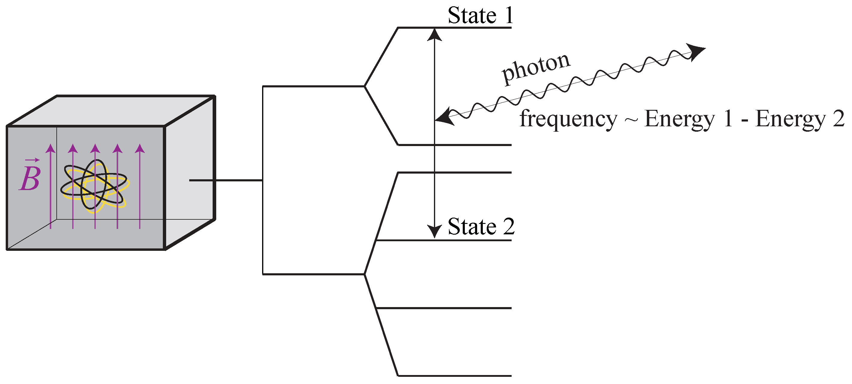
In the context of this article, a “clock” is built from an atom in a uniform magnetic field , as shown in Figure 1. Due to the the Zeeman effect and the structure of the atom itself (possibly including electron-nucleus interactions), each clock atom has a ladder of possible energy levels. The clock frequency is given by the frequency associated with a transition between a pair of energy levels in the atom, typically measured through emission or absorption of light.
When considering Lorentz-violation tests, these clocks have three important facets:
- Frequency measurements can probe atomic energy levels.
- The applied magnetic field defines an orientation of the clock: the “clock axis”.
- In conventional (i.e., Lorentz-symmetric) physics, the clock frequency is independent of the clock axis and the clock velocity.
These points, especially the third, allow us to use atomic clocks to probe Lorentz violation. Suppose that the frequency of a given clock is found to depend on its orientation. This implies a violation of rotational symmetry. Since rotations form a subgroup of the Lorentz group, this then implies a violation of Lorentz symmetry. Similarly, a clock frequency that depends on the clock’s velocity would imply a violation of boost symmetry in the Lorentz group.
This, then, is the key connection between the Lorentz-violating standard-model extension and clock-comparison experiments. If certain Lorentz-violation coefficients are nonzero, then some atomic clocks will have frame-dependent energy-level shifts. The experiments seek such frame-dependent shifts.
To date, no such frame-dependent shifts have been observed. All experiments thus place bounds on (combinations of) SME coefficients. The remainder of this paper describes the predicted energy-level shifts in detail and derives the resultant bounds on SME coefficients from existing experiments.
3. Derivation of Nonrelativistic Hamiltonian
For working with atomic states, we would like to find an appropriate nonrelativistic Hamiltonian that describes SME effects at low energies. Our pathway to doing so is to start with a relativistic Lagrangian, to use it to extract a relativistic Hamiltonian and, finally, to perform a Foldy–Wouthuysen transformation. We initially calculate a nonrelativistic Hamiltonian for free fermions; in Section 4, we discuss the sense in which the free-particle Hamiltonian may be used to describe low-energy effects on bound particles.
Throughout this paper, we restrict attention to the minimal standard-model extension in flat spacetime [6,7]. One of the primary postulates of this framework is that each free Dirac fermion of mass m is described by a Lagrangian density of the form:
where Dirac matrices M and are defined by:
In the flat-spacetime limit of the minimal SME, the coefficients , , , , , , and are fixed background tensors. They may arise, for example, as vacuum expectation values of dynamic fields in some more fundamental theory [28]. We assume in this work that each component of each coefficient tensor is much smaller than any other quantities of the same dimensions; specifically, we assume that we may neglect any terms that are higher than first order in them.
Equation (1) and many others assume the following conventions: Spacetime coordinates 0, 1, 2, 3 are denoted by Greek indices, while spatial coordinates 1, 2, 3 are denoted by Latin indices near the middle of the alphabet. The (flat) spacetime metric is , and is the free-particle momentum operator. We use the Dirac representation of the gamma matrices:
where the usual Pauli matrices are denoted by and is the identity matrix. We define the Levi–Civita symbol so that , which corresponds to the choice .
3.1. Field Redefinition
We may apply the Euler–Lagrange equations to the Lagrangian Equation (1) and then arrange the result into the form to calculate a relativistic Hamiltonian . However, the Hamiltonian that results is non-Hermitian. Interpretation of a field governed by a non-Hermitian Hamiltonian is possible [29], but problematic, so we take a different approach. The non-hermiticity arises essentially from the appearance of the nonstandard terms involving in Lagrangian Equation (1); it would not occur if . We therefore perform a field redefinition into a field basis where these coefficients are each zero before applying the Euler-Lagrange equations. With the choice [30,31]:
the field obeys conventional time evolution. Thus, the Hamiltonian extracted from will be Hermitian.
At the end of this process, the relativistic Hamiltonian takes the form:
where:
3.2. Foldy–Wouthuysen Transformation
At this point, it is best to do two fairly natural things: First, we think of our 4 × 4 matrices as 2 × 2 block matrices with each block being an ordinary 2 × 2 matrix. In this context, we incorporate the specific set of gamma matrices stated earlier: and . Once we do this, several results follow.
- The relativistic Hamiltonian is divided into block-diagonal and off-block-diagonal parts: and are block diagonal, while and are off block diagonal.
- In the nonrelativistic limit, the upper two components of satisfy a version of the Schrödinger equation with spin.
- In the nonrelativistic limit, the lower two components of are smaller than the upper components by a factor of .
- The off-block-diagonal terms in the Hamiltonian couple the upper and lower components of together. Such terms are unsuppressed by factors of , and so, we cannot immediately neglect them.
If the lower components were not coupled to the upper components, then we could simply disregard them in the nonrelativistic limit. This suggests the strategy of the Foldy–Wouthuysen transformation [32]: transform to a basis in which:
- The lower components of are still suppressed with respect to the upper components by multiple factors of .
- The Hamiltonian is approximately block diagonal. That is, the off-block-diagonal parts are suppressed with respect to the upper-left block by multiple factors of .
Symbolically, we want to find a matrix S such that:
A transformation that does the job is:
This transformation may not be calculated exactly, but may be approximated to any desired order in . Once we do so, the resulting Hamiltonian is given by an infinite power series in . In this work, we apply Equation (7) with sufficient precision that the off-diagonal blocks and lower-right block are smaller than the upper-left block by factors of . We then keep only terms up to order , and therefore, we only need keep the upper-left 2 × 2 block for describing nonrelativistic particles. The result is:
where is the conventional free-particle nonrelativistic Hamiltonian, and the Lorentz-violating perturbation is given by:
This is the Hamiltonian that we may use to calculate perturbations to energy levels of electrons, protons and neutrons in atoms.
4. Useful Assumptions and Approximations
4.1. Use of Free-Particle Perturbation
It is reasonable to be skeptical about the use of a free-particle Hamiltonian to study particles bound in atoms. Stated more precisely, an ideal Hamiltonian would take the form:
where is the full conventional Hamiltonian including atomic forces, nuclear forces and interactions with external fields; is the SME free-particle perturbation given above; and contains the SME perturbations to all interaction terms. We are omitting .
The omitted piece contains, for example, a term proportional to . By dimensional analysis, this term must also have a factor of . The resulting terms for nuclear, atomic and external magnetic fields are then suppressed by factors:
relative to the free-particle terms involving . This indicates that such terms are much smaller than the free-particle terms we are including.
We can make a somewhat more systematic argument as follows. The omitted piece is an analytic function of all quantities (except mass and angular momenta) around zero values, so it is well approximated by a multivariable Taylor series in these quantities. Applying dimensional analysis to possible terms suggests that each term is suppressed with respect to the free-particle terms, and therefore, we are keeping the largest effects.
4.2. Atomic and Nuclear Models
For unperturbed states of atoms, we use fairly rough approximations. First, we assume that electrons, neutrons and protons fall into shells. Filled shells are spherically symmetric and therefore insensitive to rotation-violating perturbations to leading order. We can therefore ignore all particles that occupy filled shells.
In most of our analysis, we make an even rougher approximation with the Schmidt model. This assumes that the dominant energy shift for each particle species comes from a single valence electron, neutron and/or proton. It then requires that the single valence particle carry all of the nuclear or electronic angular momentum.
For example, Cs contains 78 neutrons, 55 protons and 55 electrons. It has a nuclear spin and an electronic spin of . According to our model, Cs is insensitive to neutron-associated Lorentz violation. The proton-associated Lorentz-violating energy-level shift may be calculated by perturbing a single proton in a state, and the electron-associated Lorentz-violating energy-level shift may be calculated by perturbing a single electron in an state.
This model is not sophisticated, and the results should be interpreted as correct only within an order of magnitude (at best). Were Lorentz-violation to be observed in nature, then more detailed analysis would be necessary. However, in the absence of observed Lorentz-violation, analysis that identifies likely leading-order signals is sufficient.
Some work has been done in using a more realistic nuclear model to determine some energy shifts with more precision [23]. More sophisticated modeling may reveal that an energy shift that appears to be independent of a particular particle species in our simple model is in fact dependent on that species in reality [27,33].
5. Energy-Level Shifts to Atoms
To calculate atomic energy-level shifts, we treat an atom as a collection of individual particles:
where w designates each particle species, gives the number of each particle species present in a given atom and describes the Hamiltonian perturbation (9) acting on particle N of species w. As usual with perturbation theory, the first-order energy-level shift to an atomic state is given by the expectation value of in that state (F and here represent total atomic spin and spin projection, respectively). In most cases, has only one or two nonzero terms due to our use of nuclear and atomic Schmidt models.
Evaluation of the nonzero terms is aided greatly by the Wigner–Eckart theorem, which is stated in terms of tensor operators (for example, the operator is the component of rank-1tensor operator , is the component and is the component). The theorem says that the matrix element of such an operator between states and is given by:
where are the usual Clebsch–Gordon coefficients. This expression allows us to reduce the calculation of expectation values for multiple related states to simple geometry (the Clebsch–Gordon coefficients) and a single detailed expectation-value calculation.
Application of the Wigner–Eckart theorem to perturbation Hamiltonian Equation (9) then requires to be expanded in the basis of rotational tensors. For example, the term may be written:
where, as stated above, the operator is the component of rank-1 tensor operator , is the component and is the component.
Once we make this expansion in terms of tensor operators, many simplifications occur. First, we need only do a single detailed calculation—the expectation value of the part in the extreme state —for the entire operator sum and multiple states. The expectation values of the other parts in other states follow immediately from Equation (13). Next, only components contribute nonzero values as and for expectation values. Finally, the relevant Clebsch–Gordon ratios for tensor operators that appear in our Hamiltonian perturbation are fairly simple:
Putting these ideas together, we find that the expectation value of the entire perturbation Hamiltonian in state can be written:
where the dipole-type and quadrupole-type energy shifts:
Each of these expectation values is taken in the state . The tilde quantities are the combinations of Lorentz-violation coefficients that may be probed with clock-comparison experiments in ordinary matter:
Note that there is a separate set of these for each particle species even though the explicit index is not shown.
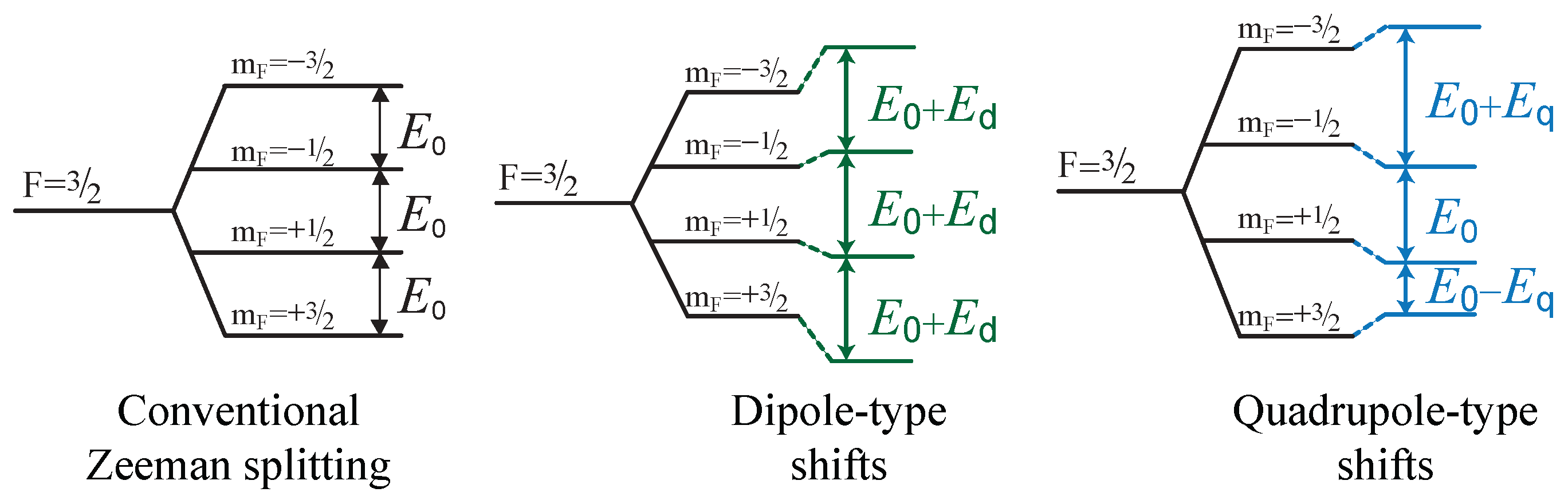
The effects of these energy shifts are qualitatively summarized in Figure 2 with the example of a multiplet. As illustrated in the figure, the most relevant quantities for comparison to experiment are transition frequencies, which are each proportional to a difference of energies. Note that dipole-type shifts are qualitatively similar to Zeeman splitting in that transitions between adjacent energy levels have equal frequencies. Quadrupole-type shifts are qualitatively different: if they are nonzero, then what appears to be a single peak in the spectrum is actually a triple peak with peak separation of size . Investigations of this effect [8,9] were early inspiration for some of the modern clock-comparison experiments.
6. Relating Theory to Experiments
A key technique for achieving high sensitivity to Lorentz-violation is watching for frequency changes as a clock’s orientation and/or velocity changes. There are two large difficulties with this. First, it is impossible to tell whether a single clock’s frequency varies or not. Second, Earth’s magnetic field can mimic Lorentz-violation: as a clock moves through Earth’s field, its frequency can vary with orientation and velocity even in conventional physics through the Zeeman effect.
Both of these problems can be solved through the introduction of the quantity [34]. Consider two co-located clocks P and Q with frequencies and . We wish to find a combination of these frequencies that is identically zero in conventional physics and that varies with orientation/velocity in the SME.
First, write each frequency in the form:
where is the conventional frequency as a function of the applied magnetic field and is the Lorentz-violating perturbation to this frequency. For example, might be expressed as for a purely electronic transition, and is a linear combination of Lorentz-violation tilde coefficients , …, . We may think of as an effective magnetic field measured by each clock, and hence, may be called a magnetometer function.
The combination is then defined to be:
The theoretical value of this quantity may be seen by expanding the magnetometer functions in Taylor series about , with the result:
where:
is proportional to the ratio of the gyromagnetic ratios for the individual frequencies. This is clearly zero in conventional physics since each is a linear combination of Lorentz-violation coefficients.
For example, suppose both clocks involve purely electronic transitions as described above. Then, . When this is plugged into Equation (20), the Lorentz-respecting terms cancel, and we find .
The experimental value of may be seen by considering two possible experimental strategies. For the first strategy, measure both and . Plug the results into and compare the result to the theoretical prediction . This strategy could work in principle, but it requires exquisitely precise knowledge of the functions and to achieve high sensitivity.
It is better to achieve high sensitivity without needing to know the magnetometer functions explicitly. For the second strategy [13], force frequency to be constant, e.g., through the application of a feedback magnetic field, and measure changes in . Then, the term is automatically constant, and so, alone contains all of the orientation/velocity dependence of . Thus,
We cannot know the value of the last piece without exquisite knowledge of and , but it is constant and so irrelevant for clock-comparison tests. In conclusion, using the second strategy with implies that orientation/velocity dependence in is sensitive purely to honest Lorentz-violating effects and , do not need to be known with much precision.
7. Time Variation
Most clock-comparison experiments to date have been conducted by probing the frequencies of interest as Earth rotates. We discuss the resulting time dependence of in this section. We also discuss the possibility of conducting a clock-comparison experiment on an orbiting platform, which could hold several significant advantages over Earth-based tests.
7.1. Earth-Based Experiments
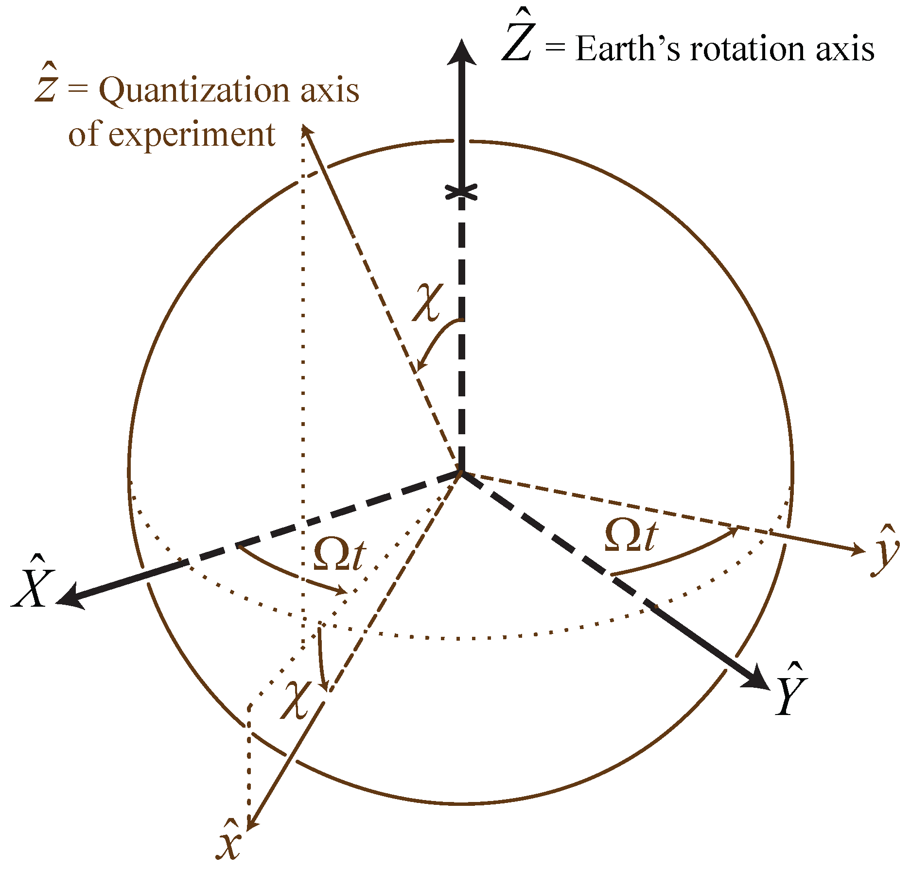
The background tensor fields themselves are commonly assumed to not vary with time or position. However, the laboratory frame changes orientation and velocity as Earth rotates, and therefore, the components of the background fields in the Earth-based reference frame vary. To extract the nature of the variation, it is useful to consider two different reference frames [27,34], as illustrated in Figure 3.
In the nonrotating frame, the origin lies at the center of the Sun. The axis is defined to be parallel to Earth’s rotation axis; the axis points toward the vernal equinox on the celestial sphere; and we choose so that the system is right-handed. When necessary, time T in the nonrotating frame is conventionally chosen so that at the vernal equinox in the year 2000. This frame is approximately inertial on time scales of thousands of years. Note that the plane coincides with Earth’s equatorial plane.
In the Earth-based frame, the origin lies at the location of the atoms involved. The axis lies along the quantization axis of the experiment. If is parallel to , then the clock orientations do not actually vary as Earth rotates, and so, there is no experimental signal. We therefore assume that makes a nonzero angle with . Then, z rotates around Z at Earth’s sidereal frequency .
We choose time to be any convenient time such that lies between and . We then pick at to lie in the plane, to be perpendicular to and to make an acute angle with . Finally, we choose so that the Earth-based frame is also right-handed. Note that maintains a constant angle with the plane and lies in the plane at all times.
Even though the frames’ origins are distinct, they are shown coincident in Figure 3 for the ease of comparison.
Given these frames, the time dependence of each Lorentz-violation coefficient may be made explicit. The combinations that appear in dipole-type energy shifts are:
while the combinations that appear in quadrupole-type energy shifts are:
The nonrotating-frame tilde quantities that appear in these expressions are linear combinations of Cartesian components of SME coefficients in the nonrotating frame. They are defined explicitly in the data tables [4]. Note that a few of the tilde-combinations received names different from their originals [27] when boost effects were no longer neglected [34]. The particular name changes were , , , , and .
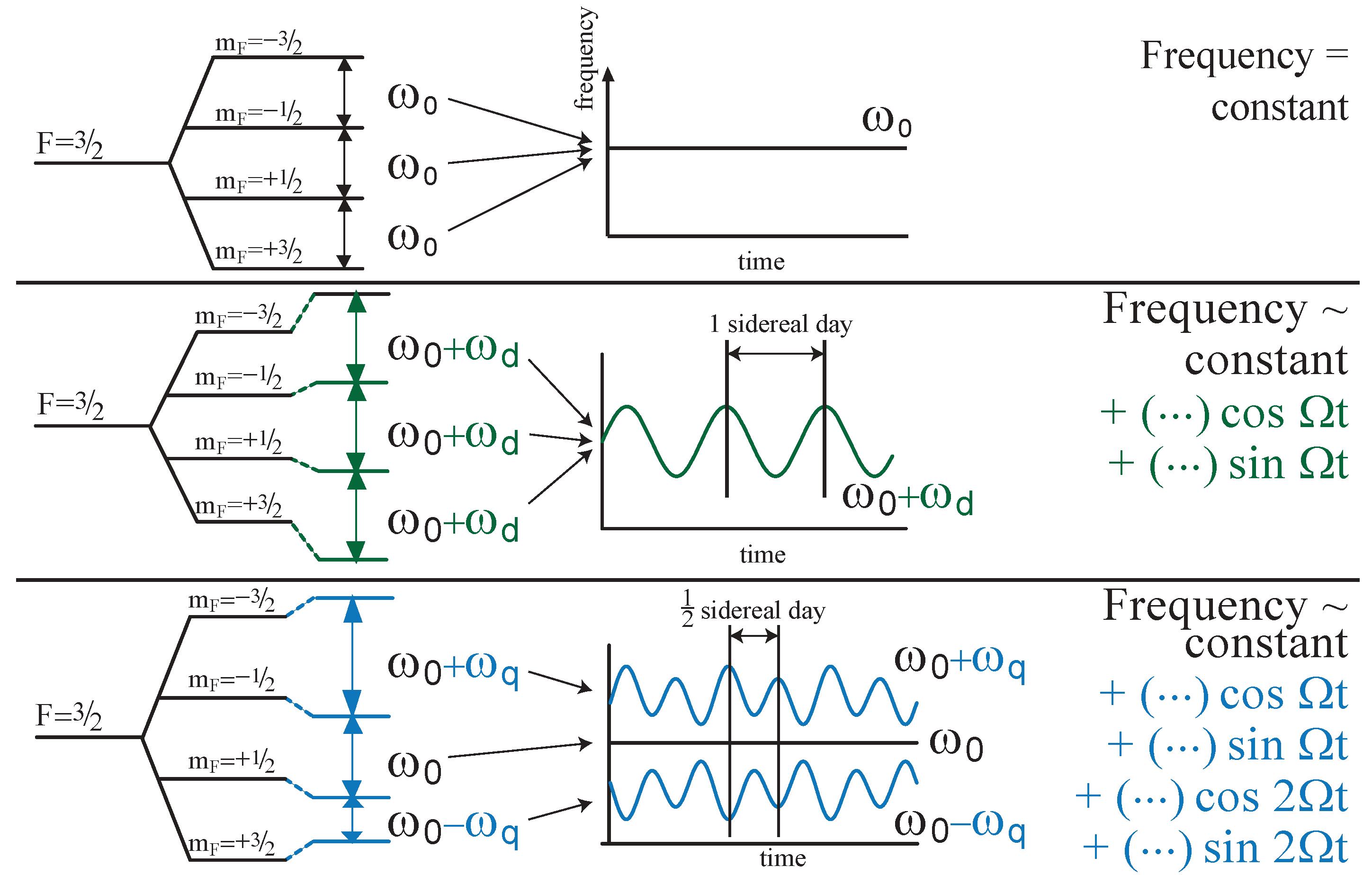
Note that the dipole-type shifts have unsuppressed variation at Earth’s sidereal frequency , while the quadrupole-type shifts have unsuppressed variation at both and . These are the only time dependencies that appear if we approximate the lab’s speed with respect to Earth’s center and Earth’s speed with respect to the Sun to be zero. If we were to keep terms of first order in each , then we would find additional contributions. Time-like nonrotating-frame components would contribute to sidereal variation suppressed by and/or . Both time-like nonrotating-frame components and dipole-type shifts would also contribute to twice-sidereal variation, also suppressed by and/or . We do not explicitly show these contributions in the current work, but they may be found elsewhere [34].
The dominant time dependencies are qualitatively summarized in Figure 4.
7.2. Space-Based Experiments
No space-based clock-comparison experiments have been performed to date. However, if performed, then experiments placed on Earth-orbiting satellites could have several advantages over experiments bound to Earth’s surface [34,35].
The first advantage is due to the freedom of satellite orbit orientation. Most surface-based experiments are forced to rotate around the same axis, Earth’s rotational axis. Energy shifts depend on relative orientations; for example, the dominant shift associated with is proportional to the dot product between and the clock axis. If happens to lie along Earth’s rotation axis, then is constant as Earth rotates and therefore undetectable in Earth-based clock-comparison experiments. Equivalently, we may say that Earth-based experiments are only sensitive to effects that are orthogonal to Earth’s rotation axis. On the other hand, space-based experiments may rotate around arbitrary axes and, therefore, may be sensitive to effects with any orientation.
The second main advantage of a satellite-based experiment would rely on the short orbital periods of many satellites. For an Earth-based experiment, a single rotation requires an entire (sidereal) day, and so, 16 rotations require 16 days to pass. Clock stability is often difficult to maintain for extended times, so 16 continual rotations may be difficult to measure. Many satellites have much shorter orbital periods. For example, a satellite in low Earth orbit has a period of about 90 min, and so, a space-based experiment may collect 16 rotations worth of data in just a single day.
The third advantage is connected with relative speeds. Several contributions to time-varying energy shifts are suppressed by a factor of about due to the low speed of Earth’s surface with respect to its center. Similar effects in satellites are suppressed less. For example, an experiment in low Earth orbit would have these boost effects suppressed by only about , a 15-fold improvement in sensitivity.
Satellite-based experiments could also have several other technical advantages. For example, satellites spend most of their time in free fall, so effective gravitational effects are only about -times as strong as on Earth’s surface. This is advantageous for fountain clocks and possibly other types. There is also likely to be less vibrational noise due to the isolation of satellites from outside influences.
The time variation of energy shifts in space-based experiments would be similar to the variation in Earth-based experiments with Earth’s sidereal frequency replaced by the satellite’s orbital frequency. However, explicit expressions for time variation of the energy shifts are much more complicated due to the many possible configurations of satellite orbits and the increased relevance of boost effects. We do not include any such explicit formulas here, but they may be found elsewhere [34].
8. Results of Completed Experiments
Table 1 lists the results of 16 completed clock-comparison experiments. Due to the difficulty in precisely calculating many nuclear and atomic expectation values, most bounds listed should be viewed as having an uncertainty of about one order of magnitude.
Many bounds include linear combinations of multiple SME tilde-coefficients. In Table 1, we simply assume that a bound on a combination implies a bound on each of the tilde-coefficients that appears. If one desires more rigorous isolation of coefficients, it is sometimes possible to combine results from multiple bounds to extract stronger bounds on the individual tilde-coefficients [36] or even separate different parts within the tilde-coefficients [37]. Due to the ongoing nature of Lorentz-violation tests, there are likely to be more opportunities of this nature in the next few years.
Acknowledgments
Thanks to Berry College and the Indiana University Center for Spacetime Symmetries for financial support during the creation of this work.
Conflicts of Interest
The author declares no conflict of interest.
References
- Einstein, A. Zur Elektrodynamik bewegter Körper. Ann. Phys. 1905, 17, 891–921. [Google Scholar] [CrossRef]
- Lorentz, H.A. Electromagnetic phenomena in a system moving with any velocity smaller than that of light. Proc. R. Neth. Acad. Arts Sci. 1904, 6, 809–831. [Google Scholar]
- Will, C.M. Was Einstein Right? Testing Relativity at the Centenary. Ann. Phys. 2006, 15, 19–33. [Google Scholar] [CrossRef]
- Kostelecky, V.A.; Russell, N. Data Tables for Lorentz and CPT Violation. Rev. Mod. Phys. 2011, 83, 11. [Google Scholar] [CrossRef]
- Kostelecky, V.A.; Potting, R. CPT, strings, and meson factories. Phys. Rev. D 1995, 51, 3923–3935. [Google Scholar] [CrossRef]
- Colladay, D.; Kostelecky, V.A. CPT violation and the standard model. Phys. Rev. D 1997, 55, 6760–6774. [Google Scholar] [CrossRef]
- Colladay, D.; Kostelecky, V.A. Lorentz violating extension of the standard model. Phys. Rev. D 1998, 58. [Google Scholar] [CrossRef]
- Hughes, V.W.; Robinson, H.G.; Beltran-Lopez, V. Upper Limit for the Anisotropy of Inertial Mass from Nuclear Re sonance Experiments. Phys. Rev. Lett. 1960, 4, 342–344. [Google Scholar] [CrossRef]
- Drever, R.W.P. A search for anisotropy of inertial mass using a free precession technique. Philos. Mag. 1961, 6, 683–687. [Google Scholar] [CrossRef]
- Prestage, J.D.; Bollinger, J.J.; Itano, W.M.; Wineland, D.J. Limits for spatial anisotropy by use of nuclear spin polarized Be-9+ ions. Phys. Rev. Lett. 1985, 54, 2387–2390. [Google Scholar] [CrossRef] [PubMed]
- Lamoreaux, S.K.; Jacobs, J.P.; Heckel, B.R.; Raab, F.J.; Fortson, E.N. New limits on spatial anisotropy from optically pumped He-201 and Hg-199. Phys. Rev. Lett. 1986, 57, 3125–3128. [Google Scholar] [CrossRef] [PubMed]
- Chupp, T.E.; Hoare, R.J.; Loveman, R.A.; Thompson, A.K. Results of a new test of local Lorentz invariance: A Search for mass anissotropy in Ne-21. Phys. Rev. Lett. 1989, 63, 1541–1545. [Google Scholar] [CrossRef] [PubMed]
- Berglund, C.J.; Hunter, L.R.; Krause, D., Jr.; Prigge, E.O.; Ronfeldt, M.S.; Lamoreaux, S.K. New Limits on Local Lorentz Invariance from Hg and Cs Magnetometers. Phys. Rev. Lett. 1995, 75, 1879–1882. [Google Scholar] [CrossRef] [PubMed]
- Bear, D.; Stoner, R.E.; Walsworth, R.L.; Kostelecky, V.A.; Lane, C.D. Limit on Lorentz and CPT violation of the neutron using a two species noble gas maser. Phys. Rev. Lett. 2000, 85, 5038–5041. [Google Scholar] [CrossRef] [PubMed]
- Phillips, D.F.; Humphrey, M.A.; Mattison, E.M.; Stoner, R.E.; Vessot, R.F.C.; Walsworth, R.L. Limit on Lorentz and CPT violation of the proton using a hydrogen maser. Phys. Rev. D 2001, 63. [Google Scholar] [CrossRef]
- Humphrey, M.A.; Phillips, D.F.; Mattison, E.M.; Vessot, R.F.C.; Stoner, R.E.; Walsworth, R.L. Testing Lorentz and CPT symmetry with hydrogen masers. Phys. Rev. A 2003, 68. [Google Scholar] [CrossRef]
- Canè, F.; Bear, D.; Phillips, D.F.; Rosen, M.S.; Smallwood, C.L.; Stoner, R.E.; Walsworth, R.L.; Alan Kostelecký, V. Bound on Lorentz and CPT violating boost effects for the neutron. Phys. Rev. Lett. 2004, 93. [Google Scholar] [CrossRef] [PubMed]
- Wolf, P.; Chapelet, F.; Bize, S.; Clairon, A. Cold atom clock test of Lorentz invariance in the matter sector. Phys. Rev. Lett. 2006, 96. [Google Scholar] [CrossRef] [PubMed]
- Kornack, T.W.; Vasilakis, G.; Romalis, M.V. Preliminary Results from a Test of CPT and Lorentz Symmetry using a K-3He Co-magnetometer. In Proceedings of the Fourth Meeting on CPT and Lorentz Symmetry, Bloomington, IN, USA, 8–11 August 2007; Kostelecký, V.A., Ed.; World Scientific: Singapore, 2008; pp. 206–213. [Google Scholar]
- Brown, J.M.; Smullin, S.J.; Kornack, T.W.; Romalis, M.V. New limit on Lorentz and CPT-violating neutron spin interactions. Phys. Rev. Lett. 2010, 105. [Google Scholar] [CrossRef] [PubMed]
- Gemmel, C.; Heil, W.; Karpuk, S.; Lenz, K.; Sobolev, Y.; Tullney, K.; Burghoff, M.; Kilian, W.; Knappe-Grüneberg, S.; Müller, W.; et al. Limit on Lorentz and CPT violation of the bound Neutron Using a Free Precession 3He/129Xe co-magnetometer. Phys. Rev. D 2010, 82. [Google Scholar] [CrossRef]
- Smiciklas, M.; Brown, J.M.; Cheuk, L.W.; Romalis, M.V. A new test of local Lorentz invariance using 21Ne-Rb-K comagnetometer. Phys. Rev. Lett. 2011, 107. [Google Scholar] [CrossRef] [PubMed]
- Flambaum, V.V. Enhancing the effect of Lorentz invariance and Einstein’s Equivalence principle violation in nuclei and atoms. Phys. Rev. Lett. 2016, 117. [Google Scholar] [CrossRef] [PubMed]
- Peck, S.K.; Kim, D.K.; Stein, D.; Orbaker, D.; Foss, A.; Hummon, M.T.; Hunter, L.R. Limits on local Lorentz invariance in mercury and cesium. Phys. Rev. A 2012, 86. [Google Scholar] [CrossRef]
- Hohensee, M.A.; Leefer, N.; Budker, D.; Harabati, C.; Dzuba, V.A.; Flambaum, V.V. Limits on violations of Lorentz symmetry and the Einstein Equivalence principle using radio-frequency spectroscopy of atomic dysprosium. Phys. Rev. Lett. 2013, 111. [Google Scholar] [CrossRef] [PubMed]
- Allmendinger, F.; Heil, W.; Karpuk, S.; Kilian, W.; Scharth, A.; Schmidt, U.; Schnabel, A.; Sobolev, U.; Tullney, K. New Limit on Lorentz-Invariance- and CPT-Violating Neutron Spin Interactions Using a Free-Spin-Precession 3He-129Xe Comagnetometer. Phys. Rev. Lett. 2014, 112. [Google Scholar] [CrossRef] [PubMed]
- Kostelecky, V.A.; Lane, C.D. Constraints on Lorentz violation from clock comparison experiments. Phys. Rev. D 1999, 60. [Google Scholar] [CrossRef]
- Kostelecky, V.A.; Samuel, S. Spontaneous breaking of Lorentz symmetry in string theory. Phys. Rev. D 1989, 39, 683–685. [Google Scholar] [CrossRef]
- Parker, L. One electron atom as a probe of space-time curvature. Phys. Rev. D 1980, 22. [Google Scholar] [CrossRef]
- Kostelecky, V.A.; Lane, C.D. Nonrelativistic quantum Hamiltonian for Lorentz violation. J. Math. Phys. 1999, 40, 6245. [Google Scholar] [CrossRef]
- Lehnert, R. Dirac theory within the standard model extension. J. Math. Phys. 2004, 45, 3399. [Google Scholar] [CrossRef]
- Foldy, L.L.; Wouthuysen, S.A. On the Dirac theory of spin 1/2 particle and its nonrelativistic limit. Phys. Rev. 1950, 78. [Google Scholar] [CrossRef]
- Brown, B.A.; Bertsch, G.F.; Robledo, L.M.; Romalis, M.V.; Zelevinsky, V. Nuclear Matrix Elements for Tests of Fundamental Symmetries. In Proceedings of the Seventh Meeting on CPT and Lorentz Symmetry, Bloomington, IN, USA, 20–24 June 2016; Kostelecký, V.A., Ed.; World Scientific: Singapore, 2017; pp. 61–64. [Google Scholar]
- Bluhm, R.; Kostelecky, A.; Lane, C.; Russell, N. Probing Lorentz and CPT violation with space based experiments. Phys. Rev. D 2003, 68. [Google Scholar] [CrossRef]
- Bluhm, R.; Kostelecký, V.A.; Lane, C.D.; Russell, N. Clock comparison tests of Lorentz and CPT symmetry in space. Phys. Rev. Lett. 2002, 88. [Google Scholar] [CrossRef] [PubMed]
- Amandolia, K.A.; Lane, C.D. Untangling coefficients for Lorentz violation. J. Young Investig. 2017, in press. [Google Scholar]
- Altschul, B. Disentangling forms of Lorentz violation with complementary clock comparison experiments. Phys. Rev. D 2009, 79, 061702. [Google Scholar] [CrossRef]
- Carroll, S.M.; Harvey, J.A.; Kostelecky, V.A.; Lane, C.D.; Okamoto, T. Noncommutative field theory and Lorentz violation. Phys. Rev. Lett. 2001, 87. [Google Scholar] [CrossRef] [PubMed]
- Lane, C.D. Spacetime variation of Lorentz-violation coefficients at a nonrelativistic scale. Phys. Rev. D 2016, 94. [Google Scholar] [CrossRef]
Figure 1.
Basic schematic of a typical atomic clock referenced in this paper. The clock’s frequency is determined by a pair of energy levels of an atom in an applied magnetic field.
Figure 1.
Basic schematic of a typical atomic clock referenced in this paper. The clock’s frequency is determined by a pair of energy levels of an atom in an applied magnetic field.

Figure 2.
Qualitative comparison of energy-level shifts to a multiplet from the conventional Zeeman effect and from dipole- and quadrupole-type Lorentz-violating operators.
Figure 2.
Qualitative comparison of energy-level shifts to a multiplet from the conventional Zeeman effect and from dipole- and quadrupole-type Lorentz-violating operators.

Figure 3.
Definition of two coordinate frames, one Sun-centered and nonrotating, the other fixed on Earth’s surface. We have drawn the frames as though they had the same origin.
Figure 3.
Definition of two coordinate frames, one Sun-centered and nonrotating, the other fixed on Earth’s surface. We have drawn the frames as though they had the same origin.

Figure 4.
Time variation of frequencies in an example system. At the top, the variation of conventional frequencies are shown for comparison, followed by variation of dipole-type energy shifts in the center and quadrupole-type energy shifts at the bottom. Effects that are suppressed by factors of have been neglected.

Table 1.
List of completed clock-comparison experiments to date with very rough bounds accomplished. The first two columns identify the experiment. The third column lists the atomic species involved. The fourth column states which SME tilde-coefficients appear in bounds. In most cases, each bound is placed on a linear combination of these coefficients with weights of order one. The final column gives the order-of-magnitude of the bound placed on the tilde coefficients listed, each of which has units of GeV. For example, the first row states that the experiment of Prestage et al. published in 1985 compared transitions in beryllium and hydrogen atoms. It bounded and associated with the neutron to each be smaller than about GeV.
| Experiment | Ref. | Atom(s) | Coefficients Bounded | |
|---|---|---|---|---|
| Prestage et al. 1985 | [10] | |||
| Lamoreaux et al. 1986 | [11] | |||
| Chupp et al. 1989 | [12] | |||
| Berglund et al. 1995 | [13] | |||
| Bear et al. 2000 | [14] | |||
| Phillips et al. 2001 | [15] | |||
| Humphrey et al. 2003 | [16] | |||
| Canè et al. 2004 | [17] | |||
| Wolf et al. 2006 | [18] | |||
| Kornack et al. 2008 | [19] | |||
| Brown et al. 2010 | [20] | |||
| Gemmel et al. 2010 | [21] | |||
| Smiciklas et al. 2011 | [22,23] | |||
| [22] | ||||
| Peck et al. 2012 | [24] | |||
| Hohensee et al. 2013 | [25] | Dy | ||
| Allmendinger et al. 2014 | [26] |
© 2017 by the author. Licensee MDPI, Basel, Switzerland. This article is an open access article distributed under the terms and conditions of the Creative Commons Attribution (CC BY) license (http://creativecommons.org/licenses/by/4.0/).
Share and Cite
MDPI and ACS Style
Lane, C.D. Using Comparisons of Clock Frequencies and Sidereal Variation to Probe Lorentz Violation. Symmetry 2017, 9, 245. https://doi.org/10.3390/sym9100245
AMA Style
Lane CD. Using Comparisons of Clock Frequencies and Sidereal Variation to Probe Lorentz Violation. Symmetry. 2017; 9(10):245. https://doi.org/10.3390/sym9100245
Chicago/Turabian StyleLane, Charles D. 2017. "Using Comparisons of Clock Frequencies and Sidereal Variation to Probe Lorentz Violation" Symmetry 9, no. 10: 245. https://doi.org/10.3390/sym9100245
Note that from the first issue of 2016, this journal uses article numbers instead of page numbers. See further details here.