Valuation Fuzzy Soft Sets: A Flexible Fuzzy Soft Set Based Decision Making Procedure for the Valuation of Assets


1
BORDA Research Unit and Multidisciplinary Institute of Enterprise (IME), University of Salamanca, E37007 Salamanca, Spain
2
Department of Economics and Business, University of Almería, E04120 Almería, Spain
*
Author to whom correspondence should be addressed.
Symmetry 2017, 9(11), 253; https://doi.org/10.3390/sym9110253
Submission received: 22 September 2017
/
Revised: 23 October 2017
/
Accepted: 23 October 2017
/
Published: 27 October 2017
(This article belongs to the Special Issue Fuzzy Techniques for Decision Making)
Abstract
:Zadeh’s fuzzy set theory for imprecise or vague data has been followed by other successful models, inclusive of Molodtsov’s soft set theory and hybrid models like fuzzy soft sets. Their success has been backed up by applications to many branches like engineering, medicine, or finance. In continuation of this effort, the purpose of this paper is to put forward a versatile methodology for the valuation of goods, particularly the assessment of real state properties. In order to reach this target, we develop the concept of (partial) valuation fuzzy soft set and introduce the novel problem of data filling in partial valuation fuzzy soft sets. The use of fuzzy soft sets allows us to quantify the qualitative attributes involved in an assessment context. As a result, we illustrate the effectiveness and validity of our valuation methodology with a real case study that uses data from the Spanish real estate market. The main contribution of this paper is the implementation of a novel methodology, which allows us to assess a large variety of assets where data are heterogeneous. Our technique permits to avoid the appraiser’s subjectivity (exhibited by practitioners in housing valuation) and the well-known disadvantages of some alternative methods (such as linear multiple regression).
1. Introduction
Zadeh’s [1] fuzzy set theory deals with impreciseness or vagueness of evaluations by associating degrees to which objects belong to a set. Its appearance boosted the rise of many related theories that attempt to model specific decision problems. In particular, the hybridization of fuzzy sets with soft sets as proposed by Molodtsov [2] (see also Maji et al. [3,4]) yields the notion of fuzzy soft set (Alcantud [5], Ali [6], Ali and Shabir [7], Maji et al. [8]). Decision-making methodologies and applications have proliferated and are the subject of relevant analyses on a regular basis. Among the most recent papers that exemplify noteworthy fuzzy decision-making trends, we can cite Alcantud et al. [9,10], Faizi et al. [11,12] and Zhang and Xu [13] in hesitant fuzzy sets, Zhan and Zhu [14] in (fuzzy) soft sets and rough soft sets, Alcantud [15] in fuzzy soft sets, Ma et al. [16] in hybrid soft set models, Chen and Ye [17] and Ye [18] in neutrosophic sets, Peng et al. [19] and Peng and Yang [20] in interval-valued fuzzy soft sets, and Fatimah et al. [21] in (dual) probabilistic soft sets. With respect to applications, in a clinical environment, Chang [22] uses the fuzzy sets theory and the so-called VIKOR (VIsekriterijumska optimizacija i KOmpromisno Resenje) method to evaluate the service quality of two public and three private medical centres in Taiwan, in the same context of uncertainty, subjectivity and linguistic variables as our study; Espinilla et al. [23] apply a decision analysis tool for the early detection of preeclampsia in women at risk by using the data of a sample of pregnant women with high risk of this disease; and Alcantud et al. [24] give a methodology for glaucoma diagnosis. On the other hand, in the field of management, Zhang and Xu [13] deal with the problem of choosing material suppliers by a manufacturer to purchase key components in order to reach a competitive advantage in the market of watches; Xu and Xia [25] provide a management case study by using the hesitant fuzzy elements to estimate the degree to which an alternative satisfies a criterion in a decision-making process; Taş et al. [26] present new applications of a soft set theory and a fuzzy soft set theory to the effective management of stock-out situations. In the field of finance, Xu and Xiao [27] apply the soft set theory to select financial ratios for business failure prediction by using real data sets from Chinese listed firms; Kalaichelvi [28] and Özgür and Taş [29] apply fuzzy soft sets to solve the investment decision making problem.
In this work, we introduce the notion of partial valuation fuzzy soft set as a tool to perform valuations of assets. Then, we apply a suitable valuation methodology, based on fuzzy soft sets, to a real case study. Fuzzy soft sets, with their ability to codify partial membership with respect to a predefined list of attributes, seem to be a useful tool to make decisions in this context. Unlike the standard approach, which selects one from a set of possible alternatives, our decision is the valuation that should be rightfully attached with some of the assets. In passing, we introduce rating procedures as well as the problem of data filling in partial valuation fuzzy soft sets.
Our application concerns the real estate market. There is ample variety of real estate valuation methods. Following [30], we classify them into traditional and advanced. Traditional methods are: comparison method, investment/income capitalization method, profits method, development/residual method, contractors/cost method, multiple regression method, and stepwise regression method. As advanced valuation methods, we can cite: artificial neural networks (ANNs), hedonic pricing method, spatial analysis methods, fuzzy logic, and autoregressive integrated moving average (ARIMA).
In Spain, real estate valuation is regulated by Orden ECO/805/2003 (Ministerio de Economía, 2003) [31], which recommends the use of four of the previously mentioned methods: comparison, investment/income capitalization, residual, and cost methods. There are some interesting works that compare certain methods used in real estate appraisal, e.g., [32] compare fuzzy logic to multiple regression analysis, or [33] compare artificial-intelligence methods with non-traditional regression methods. We also find new hybrid methodologies, e.g., [34], which relies on the introduction of fuzzy mathematics in a spatial error model.
We contribute to this growing literature by proposing a flexible mechanism that can be specialized in several ways. The input data is a partial valuation fuzzy soft set that characterizes the problem. The practitioner can select one from a sample of rating procedures in order to start the algorithm. Then, a suitable regression analysis permits filling the missing data in the original partial valuation fuzzy soft set. The structure of the available data often allows the researcher to perform sophisticated regression analysis beyond the standard, linear case.
This paper is organized as follows. Section 2 recalls some notation and definitions related to soft sets and fuzzy soft sets. Section 3 presents the main new notions in this paper, namely, valuation and partial valuation fuzzy soft sets. We also define rating procedures for fuzzy soft sets and prove some useful fundamental properties of these concepts. Section 4 briefly introduces data filling for partial valuation fuzzy soft sets, and a flexible methodology is proposed in order to implement that concept. Then, in Section 5, we take advantage of such design in order to valuate goods through a fictitious streamlined example. In Section 6, we present an application to a real case study on the Spanish real estate market. We also examine its traits in comparison with other standard methodologies. We conclude in Section 7.
2. Notation and Definitions
Let X denote a set. Then, is the set of all subsets of X. A fuzzy subset (also, FS) A of X is a function . For each , is the degree of membership of x in that subset. The set of all fuzzy subsets on X will be denoted by FS(X).
Now, we are going to recall some basic concepts such as soft sets and fuzzy soft sets.
2.1. Soft Sets and Fuzzy Soft Sets
In soft set theory, we refer to a universe of objects U, and to a universal set of parameters E.
Definition 1
([2]). Let A be a subset of E. The pair is a soft set over U if .
The pair in Definition 1 is a parameterized family of subsets of U, and A represents the parameters. Then, for every parameter , we interpret that is the subset of U approximated by e, also called the set of e-approximate elements of the soft set.
Other interesting investigations expanded the knowledge about soft sets. The notions of soft equalities, intersections and unions of soft sets and soft subsets and supersets are defined in [4]. Various types of soft subsets and soft equal relations are studied in [35]. Soft set based decision-making was initiated by [3]. Further applications of soft sets in decision-making contexts were given, for example, in [24,36,37].
The concept of soft set can be expanded so as to include fuzzy subsets approximated by parameters:
Definition 2
([8]). Let A be a subset of E. The pair is a fuzzy soft set over U if , where denotes the set of all fuzzy sets on U.
The set of all fuzzy soft sets over U will be denoted as (U). Due to the natural identification of subsets of U with FSs of U, any soft set can be considered a fuzzy soft set (cf., [5]). If, for example, our universe of options are films that are parameterized by attributes, then fuzzy soft sets permit to deal with properties like “funny” or “scary” for which partial memberships are almost compulsory. However, soft sets are suitable only when properties are categorical, e.g., “Oscar awarded”, “3D version available”, or “silent movie”.
In real practice, both U and A use to be finite. Then, k and n will denote the respective number of elements of and . In such case, soft sets can be represented either by matrices or in their tabular form (cf., [38]). The k rows are associated with the objects, and the n columns are associated with the parameters. Both practical representations are binary, that is to say, all cells are either 0 or 1. One can proceed in a similar way in fuzzy soft sets, but now the possible values in the cells lie in the interval .
A matrix representation of a soft set is shown in the following Example 1:
Example 1.
Let be a universe of houses. Let be the set of parameters, attributes or house characteristics (e.g., “centrally located” or “includes a garage”). Define a soft set as follows:
- 1.
- , .
- 2.
- , .
- 3.
- , .
Table 1 captures the information defining .
Suppose that a soft set can be expressed by the matrix . Then, the choice value of object is defined as . According to Maji, Biswas and Roy [3], an optimal choice can be made by selecting any object such that . Put differently, any choice-value maximizer is an acceptable solution to the problem.
However, fuzzy soft set decision making is far more complex thus controversial. Approaches to that problem are included in [15,39,40,41].
Anyhow, the example above shows that fuzzy soft sets are a suitable tool to capture the characteristics of complex representations of assets. Section 6 below clarifies this argument with a real example.
2.2. Basic Operations
Basic operations among soft sets were established in Ali et al. [42]:
Definition 3
([42]). Let and be soft sets over U, such that . The restricted intersection of and is denoted by and it is defined as , where for all .
Definition 4
([42]). The extended intersection of the soft sets and over U is the soft set , where , and ,
It is denoted by .
Definition 5
([42]). Let and be soft sets over U, such that . The restricted union of and is denoted by and it is defined as , where and for all .
Definition 6
([42]). The extended union of two soft sets and over U is the soft set , where , and ,
It is denoted by .
Maji et al. [8] defined some relations and similar operations for fuzzy soft sets as follows.
Definition 7
([8]). Let and be fuzzy soft sets over U. We say that is a fuzzy soft subset of if and is a fuzzy subset of for all .
When is a fuzzy soft subset of and is a fuzzy soft subset of we say that and are fuzzy soft equal.
Definition 8
([8]). Let and be fuzzy soft sets over U.
Their intersection is where and for all .
Their union is , where , and ,
3. Some Novel Concepts Related to Valuation Fuzzy Soft Sets
In this section, we are going to introduce the main new notions in this paper, namely, valuation and partial valuation fuzzy soft sets. We also prove some fundamental properties of them.
Valuation and Partial Valuation Fuzzy Soft Sets
In order to define our novel notions, we refer to a universe U of k objects, and to a universal set of parameters E.
Definition 9.
Let A be a subset of E. The triple is a valuation fuzzy soft set over U when is a fuzzy soft set over U and . Henceforth, we abbreviate a valuation fuzzy soft set by VFSS. We denote by V (U) the set of all valuation fuzzy soft sets over U.
If we restrict Definition 9 to soft sets over U, a particular concept of valuation soft set is naturally produced.
The motivation for valuation (fuzzy) soft sets is that, in many natural situations, option from U is associated with a valuation, appraisal or assessment , in addition to the standard parameterization of U as a function of the attributes in A. For example, in the usual example where the options are houses, this valuation may be the market price.
Such valuation can also be defined through elements from fuzzy soft set theory, or otherwise. We proceed to formalize these ideas.
Definition 10.
A rating procedure for fuzzy soft sets with attributes A on a universe U is a mapping
Every rating procedure associates each FSS over U with a VFSS over U. For example, one can use scores associated with decision making mechanisms from the literature (e.g., fuzzy choice values, the scores computed in [39], or the refined scores computed in [15]), in order to produce particularly noteworthy rating procedures. We formalize them in the following definitions:
Definition 11.
The fuzzy choice value rating procedure is defined by the expression , where for each . Recall that is the fuzzy choice value of option i.
Definition 12.
Definition 13.
Alcantud’s rating procedure is defined by the expression , where is the score associated with option i in Algorithm 2 of [15].
In this paper, we are especially concerned with Definition 13. In order to make this paper self-contained, we proceed to recall its construction.
We describe our fuzzy soft set on k alternatives in tabular form. Let denote its cell for each possible . Now, for each parameter , let be the maximum membership value of any object (). Then, we construct a comparison matrix , where for each , is the sum of the non-negative values in the finite sequence
Of course, such matrix can also be expressed as a comparison table.
For each , let be the sum of the elements in row i of A, and be the sum of the elements in column i of A. Finally, for each , the score of object i is .
The following toy example illustrates the notions above.
Example 2.
The application of Definitions 11, 12 and 13 to produces three respective VFSSs, namely,
and
In order to obtain these results, we note that the fuzzy choice values in Definition 11, and the scores in Definition 12, are calculated in Table 6 of [40]. In addition, the scores associated with the options by Definition 13 are computed in Figure 2 of [15].
These , and scores produce the respective VFSSs above. Such VFSSs are summarized in Table 3.
In order to select a suitable rating procedure, Definition 13 is the natural choice that we recommend for the valuation of fuzzy soft sets. Our advice is based on the following arguments. Firstly, most authors agree that it seems untenable to use Definition 11, which is a simple adapted version of choice values. Although choice values are widely acceptable in soft set theory, they cannot capture the subtleties of the more general model by FSSs. Therefore, we discard Definition 11. Secondly, Definition 12 does not capture whether an alternative beats another one by a narrow or a large margin, while Definition 13 explicitly rewards more ample differences in the degree of satisfaction of the characteristics. In applications like real estate valuation, the wide range of the feasible assessments demands a method that incorporates these differences. Otherwise, the results will be affected by the odd fact that alternatives with striking differences in their characteristics should be equally valuated, which is clearly a blunt mistake. For these reasons, we must discard Definition 12 and recommend Definition 13.
For practical purposes, the following definition will be very useful. It concerns the cases where some of the valuations are unknown.
Definition 14.
Let A be a subset of E. The triple is a partial valuation fuzzy soft set over U when is a fuzzy soft set over U and . We abbreviate partial valuation fuzzy soft set by PVFSS.
The set of all partial valuation fuzzy soft sets over U will be denoted as U). If we restrict Definition 14 to soft sets over U, then we define the particular concept of partial valuation soft set. As in the case of VFSSs, each option from U is associated with a valuation in addition to the standard parameterization of U as a function of the attributes in A. However, in PVFSSs, it may happen that some of the valuations is unknown or missing. In such case we represent the unknown information or missing valuation data by the * symbol.
Now the motivation for PVFSSs goes as follows. Quite often some options from U have an intrinsic valuation (for example, market price), whereas the valuation of other options are unknown (for example, because it is our own house that we want to put up for sale). The model by PVFSSs permits collecting all that information in a concise format.
4. Data Filling in Partial Valuation Fuzzy Soft Sets
Valuation is an abstract concept that can be specialized in many ways. We can take advantage of this issue in order to fill missing data in PVFSSs through an adjustable approach. The motivation for this novel problem is the following. If there are missing valuation data in a PVFSS, then the assessments of the corresponding alternatives are unknown. Should we need them (for example, because the valuation of our house means the market price that we might expect when we put it up for sale), then we must fill the missing data.
Therefore the problem of data filling in PVFSSs is associated with solving an original decision making problem for alternatives that are characterized by FSSs.
Remark 1.
The idea of partial valuations should not be mistaken with the well-known notion of incomplete (fuzzy) soft sets [36,43,44,45,46]. In the latter case, the parameterization has missing values. In our model, the parameterization of the universe is complete, whereas the valuation is not necessarily complete. Thus, the statement of our data filling problem is original with this paper.
We proceed to define our class of procedures for the valuation of goods when (a) these goods are characterized by parameters, and (b) there are comparable goods that are characterized by the same parameters. In other words, we have information about the goods in the form of PVFSSs.
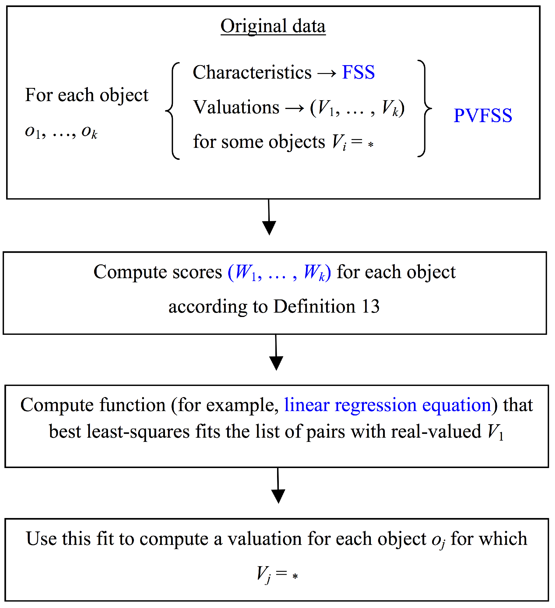
Our methodology is very direct. It works as follows. Let us select a rating procedure (cf., Definition 10).
- Let us input our PVFSS, namely, .
- We use the rating procedure in order to associate a unique number with each alternative. In this way, we obtain a VFSS associated with the same FSS as the original PVFSS.
- Now, as long as there are two values in that belong to (i.e., two valuations that are not missing in the input data), we calculate a regression equation to fill the missing valuation data.In order to run the regression, the independent variables (or abscissas) are the values given by the rating procedure that has been singled out, and the dependent variables (their respective ordinates) are the corresponding valuations.
- Once the regression function has been calculated, we can estimate the real values of the missing valuations by its evaluations in the corresponding values.
This procedure solves our original data filling problem.
This methodology is flexible because we can use any rating procedure to produce the abscissas of the data plots and also because we can use regression models other than linear regression in order to fill the missing data (step 3). Observe that in such cases we need a larger set of non-missing data.
The flowchart in Figure 1 summarizes the steps in our solution to the problem of data filling for PVFSSs.
5. Valuation of Goods: An Example
For a given a list of options characterized by a PVFSS, the information on the known values can be used to fill the missing data. Observe that at the end of the process we are valuating the assets with missing values. Therefore, we can use the data filling procedures described in Section 4 in order to make decisions e.g., as to which prizes should be attached to properties that are put into the market.
In this section, we explain this possibility with the following fully developed example. Table 4 represents a PVFSS denoted . It uses the input data of Table 6 of [15], which we complement with valuations of some of the six alternatives.
We can interpret Table 4 as follows. We are interested in selling property , whose market value we want to assess ourselves. The options include our property and other real state properties for sale, and they are all characterized by the attributes. An inspection of the market shows that recent purchases in the same area or street amounted to the respective ’s. With this practical information, we are ready to valuate our property.
Let us select the rating procedure . We are ready to apply the remaining steps in Section 4. As explained above, valuates the options by using Alcantud’s scores. Therefore,
because these figures are computed in Table 8 of [15]. Hence, the VFSS that we obtain at step 2 of our data filling solution in Section 4 is .
We now compute the linear regression equation from the bivariate data that combine the known valuations at with the corresponding components of our rating procedure in the abscissas, which yields
Observe that the values have been discarded because the valuation of the 4th alternative is missing.
Some easy computations (see for example [47]) show that the regression line equation in step 3 is
with a coefficient of determination . Figure 2 displays these computations.
Finally, in step 4, we evaluate such function at the score value associated with , which produces the evaluation value .
In conclusion, option should be valuated by euros.
6. A Real Case Study
In this section, we propose a method to appraise real estate based on fuzzy logic as we concur with [48] on “the applicability of fuzzy logic for expressing the inherent imprecision in the way that people think and make decisions about the pricing of real state”. As far as we know, no methodology based on fuzzy soft sets has ever been applied to real estate valuation using real data from the market. We here use the novel procedure that relies on the new notion of data filling in PVFSSs (as applied in Section 5) in order to provide an assessment of a property based on real data from Almería, in Southeast Spain. The data were obtained by one of the coauthors who acted as appraiser in 2016. Lastly, we compare our existing methodologies.
To be precise, for such real application, we intend to assess an apartment (the subject property) using the data of six apartments (the comparable properties), with known sale prices. We also know the values of four selected attributes (cf., Table 5): surface, number of bathrooms, quality, and number of bedrooms. The values for the attribute “surface” are expressed in square meters. Apartment 6 has bathrooms, which means that it has a complete bathroom with a bathtub and another bathroom without a bathtub. There are other attributes, like location and age that we did not include in the table because the six comparable properties and the subject property had similar values (they were located in the same area and were built approximately in the same year).
The property we have to assess has a surface of square meters, one bathroom, two bedrooms and a “good” quality.
To apply the method explained in Section 4 and Section 5, we first adapt the data to fuzzy soft set format, and, for this purpose, we perform the following adjustments:
- The maximum surface in our sample of seven apartments is 114.44 square meters. We have divided the surface of each apartment by this maximum figure.
- We have divided the number of bathrooms of each apartment by two, the maximum number of bathrooms per apartment in our sample.
- In order to rank the attribute “quality”, we have considered four levels of quality: bad, normal, good, and luxury. We assign the values and 1 to each level, respectively.
- For the attribute “number of bedrooms”, we have divided the actual number of bedrooms by the maximum number of bedrooms, which, in our sample, is four.
Table 6 shows the PVFSS that captures the statement of our real valuation problem.
6.1. Evaluation of the Apartment
If we select the rating procedure , then we first compute the comparison table associated with Table 6. Such item is given in Table 7 (the values have been rounded off for the purpose of presentation).
By Definition 13, we obtain:
These values are given by Alcantud’s scores in Table 7.
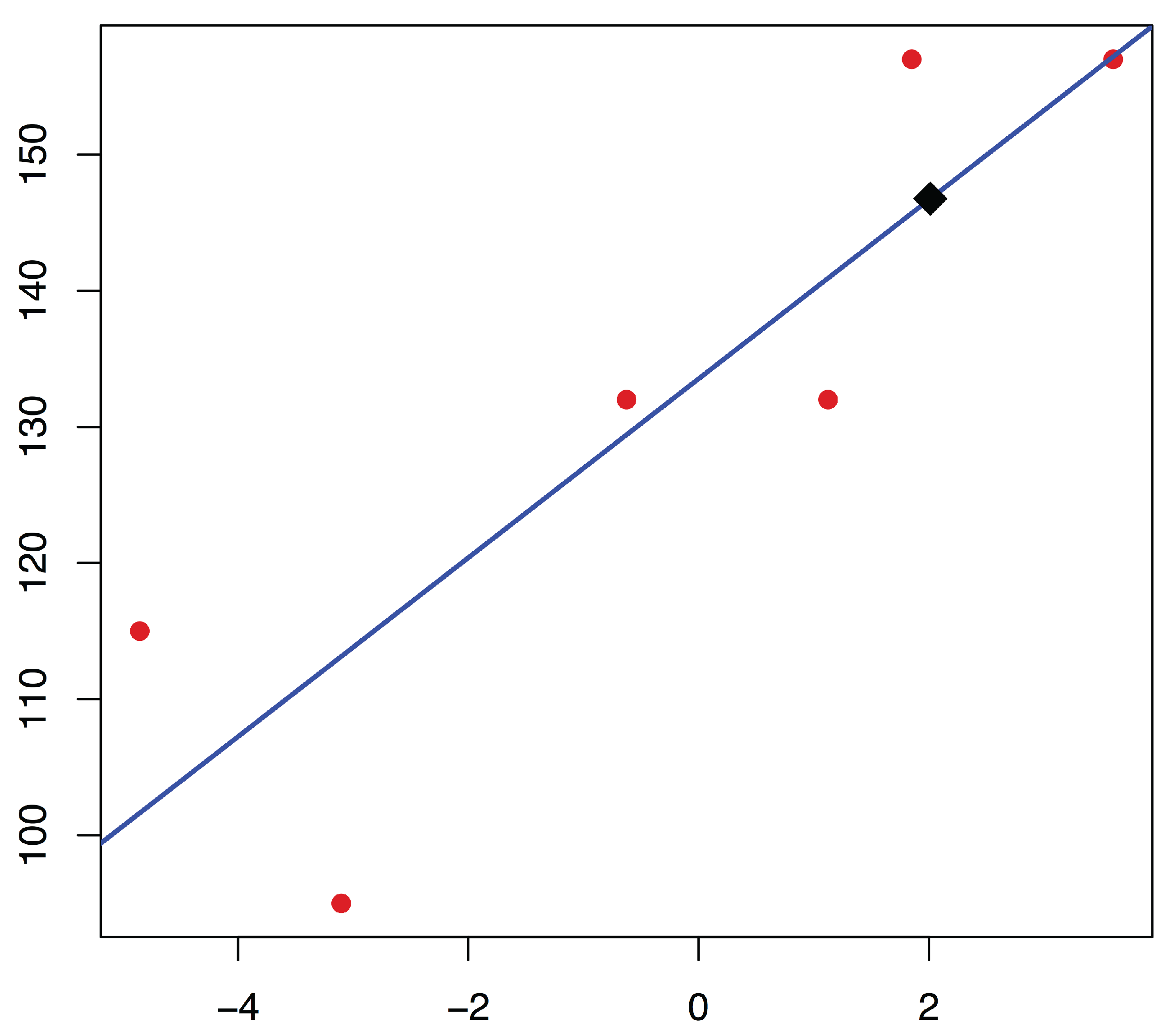
We now need to calculate the linear regression equation from the bivariate data that combine the known valuations with the corresponding components of our rating procedure, which are
Some easy computations show that the regression line equation is
where y are prices, x represent the scores, and the coefficient of determination takes an acceptable value (). Hence, for the value of the y variable is , and we conclude that the property should be priced at euros because prices were given in thousands of euros. Figure 3 displays these computations.
6.2. Sensitivity Analysis
Prices in the real estate market are subject to volatility. In addition, the appraiser can select the small sample in accordance to the existing regulations. Therefore, we have to account for some degree of uncertainty in the valuation of the subject property.
Sensitivity analysis studies how the uncertainty in the output of a mathematical model can be associated with different sources of uncertainty in its inputs [49]. The techniques of sensitivity analysis are sundry and the choice of a suitable methodology is often dictated by the structure of the model. Since we work with given data, we can screen for submodels and check how much the selection of a subsample affects the output. We proceed to check that under such variations the differences in the outputs are small, which allows us to conclude that our valuation model is fairly robust.
- When the first apartment is suppressed from the analysis, the remaining data produce a new comparison table and scores. With such data, we obtain . The regression line equation for the observationsis and substituting produces a figure of euros. Thus, the difference with respect to the original valuation, in absolute value, is only .
- When the second apartment is suppressed from the analysis, the remaining data produce . The regression line equation for the observationsis and substituting produces a figure of euros. Therefore, the difference with respect to the original valuation, in absolute value, is only .
- When the sixth apartment is suppressed from the analysis, the remaining data produce . The regression line equation for the observationsis and substituting produces a figure of euros. Therefore, the difference with respect to the original valuation, in absolute value, is only .
6.3. A Description of Existing Methodologies
In this section, we briefly sketch the standard methodologies applied by practitioners. Then, in Section 6.4 below, we compare them with the new methodology proposed in Section 6.1.
In order to estimate the price of a house, the comparison method and the multiple linear regression method are most used in real estate practice in Spain. Both techniques are based on a list of variables (either qualitative or quantitative) that describe the characteristics of the houses in the sample. These attributes of the properties may be of different types:
- Quantitative and continuous variables, such as the surface of a house.
- Quantitative and discrete variables, such as:
- Number of complete bathrooms.
- Number of incomplete bathrooms.
- Age of the building.
- Number of rooms.
- Level in which is the apartment situated in the building (floor).
- Number of outward-facing rooms, etc.
- Qualitative variables, such as quality of the construction.
- Dummy variables, such as:
- The building has a garage.
- The house has a balcony.
- Repairing and renovation works were made in the house, etc.
The comparison method assigns a positive or a negative weight to each modality presented by every attribute, depending on whether the variable must positively or negatively influence the housing price. The values of these weights are, of course, in agreement with the level of the corresponding attribute. Indeed, a given attribute k can be a discrete or a continuous quantitative variable, a qualitative variable, or a “dummy” variable.
To each value, interval modality or “dummy” value of Table 8, we can assign a weight .
If , denotes the price of the i-th apartment, its surface, and , , represents the weight assigned to the k-th attribute of the i-th element in the sample, the normalized average price of a square meter is:
Therefore,
where the subscript 0 corresponds to the house to be assessed.
The multiple linear regression method consists of regressing the variable P (price of the house) on the rest of variables involved in the valuation process, e.g.:
- : “Surface”.
- : “Number of bathrooms”.
- : “Quality”.
- : “Number of bedrooms”.
- Etcetera.
Thus, we are able to obtain a regression hyperplane in the following form:
The concrete values of variables corresponding to the house to be appraised will allow us to estimate P. Indeed, the main advantage of this method is the objectivity of the result. Unfortunately, this procedure may present two noteworthy drawbacks. First, the goodness of fit in the regression analysis can be very low, which means that the result that produces is not significant at a certain level. Second, a concrete coefficient may exhibit a “wrong” sign in the way that the estimated sign on a variable is the opposite of what we anticipated it should be. For example, it is expected that the price of a house is ceteris paribus inversely related to its age, but the practical implementation of this technique can lead to a positive coefficient for this variable. A possible solution could be to restrict the coefficients to the set of positive or negative real numbers, but, unfortunately, the coefficient of determination does not measure, in this case, the goodness of the fit.
When the linear relationship between the dependent variable (the price) and the regressors (the rest of variables involved in the analysis) has been computed, the values of the attributes of the house to be assessed are included in the equation, which produces an estimated market price. Indeed, a drawback of this method is that the goodness of fit (given by the coefficient of determination) may be very low. This is the reason why it seems convenient to find an appropriate sample (composed by, at least, six houses) for which the fitting should be acceptable.
We return to these issues in the next section.
6.4. Evaluation with Alternative Procedures and Discussion
The routine application of the multiple regression technique to the data included in Table 5 leads to the following three-dimensional hyperplane:
which leads to a price euros. Although the coefficient of determination is very high (), this outcome is rather disappointing for two main reasons. The coefficient of has the wrong sign because ceteris paribus the price of an apartment should increase both with the number of bedrooms. Moreover, observe that the coefficient of vanishes. The reason is that all the apartments with a valuation in the sample have a “normal” quality, even though there are other values for this attribute in the sample. This is another important drawback of this method since, in our real case study, such zero value implies the fact that the apartment being assessed has a “good” quality cannot be used to increase its valuation.
Let us now approximate the price of the apartment according to the weights shown in Table 9. According to the Orden ECO/805/2003 (Ministerio de Economía, 2003) [31], the coefficients to standardize the value of the square meter of each element in the sample will be chosen by applying the criteria suitable for the house to be assessed. Nevertheless, this procedure, called the homogenization method, “has got some problems which should be solved and that are related, for example, with valuer’s subjectivity” [50]. Therefore, in this paper, we have implemented the standard weights used by practitioners, which are based on a proposal by González-Nebreda et al. [51].
The application of this information to the characteristics of the apartments in the sample and the apartment to be assessed produces Table 10, where, for completeness, the price of each apartment is shown too.
By applying Formula (1), we obtain a price of 171,747.78 euros.
All in all, along this paper, we have compared three methodologies to approximate the value of an apartment from the information supplied by the housing market about the characteristics (price, surface, number of bathrooms, number of bedrooms and quality) of a sample composed by six other apartments.
The first method uses the linear multiple regression where the dependent variable is the price and the independent variables are the rest of the characteristics of the apartments. This technique is subject to at least three noteworthy inconveniences, which dramatically reduce the validity of its results:
- The possible existence of coefficients with the wrong sign (in our case, the coefficient of variable ).
- The possibility that a coefficient vanishes (in this section, the coefficient of variable is zero). In such case, the characteristic associated with the corresponding variable is of no use for evaluation purposes.
- The coefficient of determination may be small (although, in the example in this section, is pretty high).
The second procedure uses the weights assigned by practitioners to highlight the “good” characteristics of all apartments and to penalize their “bad” figures. This methodology presents an important disadvantage, viz. the enormous subjectivity in choosing these weights.
The third technique is new with this paper. It produces a much more reasonable result, which is partially due to the reduction of subjectivity in the weights.
Despite the disparities between prices, let us stress that the price finally agreed in the transaction of this apartment was much closer to the value given by the proposed methodology.
7. Conclusions
In this work, we propose the new notion of partial valuation fuzzy soft sets and we briefly introduce the problem of data filling in that setting (cf., Section 3 and Section 4). The use of fuzzy soft sets permits quantifying qualitative attributes, such as the finish of housing construction or the quality of materials used in the construction of a house. Therefore, we can apply these ideas in real estate valuations. By doing so, we depart from fuzzy soft sets and extend their scope with the target of real applications. In our approach, we first use a rating procedure in order to associate a unique number (score) with each alternative and then we apply regression for the purpose of data filling in partial valuation fuzzy soft sets (cf., Section 4). We have explained our model both algorithmically and with a flow diagram.
Then, we have shown how this new methodology works in a fictitious (cf., Section 5) and a real case study (cf., Section 6). With these examples, we have proved the implementability and feasibility of our methodology. We have also performed a sensitivity analysis in order to avail its robustness. The real case study concerns apartments. Obviously, it can be also applied in the valuation of other kind of assets, such as rural properties, cars, etc. We have obtained a very reasonable price for the house under valuation, which proves the feasibility and implementability of our suggestion. On the other hand, the two alternative methods (that were based on the linear multiple regression and used by practitioners) exhibit serious troubles that restrict their ability to fit real situations.
To conclude, let us point out that our technique can be useful for practitioners using other models of uncertain behavior. For example, the idea that scores can be used to perform a regression can easily be exported to models based on hesitant fuzzy sets [11,12,52,53,54,55] for which scores are already available [56,57,58]. It seems also feasible to export it to other hybrid soft set models (cf., Ali et al. [59], Fatimah et al. [60], Ma et al. [16], Zhan and Zhu [14], and Zhan et al. [61]).
Acknowledgments
We are grateful for the constructive comments by three anonymous referees. The second and third authors acknowledge the financial support from the Spanish Ministry of Economy, Industry and Competitiveness, and the European Regional Development Fund-ERDF/FEDER-UE (National R & D Project ECO2015-66504 and National R & D Project DER2016-76053-R).
Author Contributions
The authors contributed equally to this work.
Conflicts of Interest
The authors declare no conflict of interest.
Abbreviations
The following abbreviations are used in this manuscript:
| MDPI | Multidisciplinary Digital Publishing Institute |
| DOAJ | Directory of Open Access Journals |
| FS | Fuzzy set |
| PVFSS | Partial valuation fuzzy soft set |
| VFSS | Valuation fuzzy soft set |
| VIKOR | VIsekriterijumska optimizacija i KOmpromisno Resenje |
References
- Zadeh, L. Fuzzy sets. Inf. Control 1965, 8, 338–353. [Google Scholar] [CrossRef]
- Molodtsov, D. Soft set theory–first results. Comput. Math. Appl. 1999, 37, 19–31. [Google Scholar] [CrossRef]
- Maji, P.K.; Biswas, R.; Roy, A.R. An application of soft sets in a decision making problem. Comput. Math. Appl. 2002, 44, 1077–1083. [Google Scholar] [CrossRef]
- Maji, P.K.; Biswas, R.; Roy, A.R. Soft set theory. Comput. Math. Appl. 2003, 45, 555–562. [Google Scholar] [CrossRef]
- Alcantud, J.C.R. Some formal relationships among soft sets, fuzzy sets, and their extensions. Int. J. Approx. Reason. 2016, 68, 45–53. [Google Scholar] [CrossRef]
- Ali, M.I. A note on soft sets, rough soft sets and fuzzy soft sets. Appl. Soft Comput. 2011, 11, 3329–3332. [Google Scholar] [CrossRef]
- Ali, M.I.; Shabir, M. Logic connectives for soft sets and fuzzy soft sets. IEEE Trans. Fuzzy Syst. 2014, 22, 1431–1442. [Google Scholar] [CrossRef]
- Maji, P.K.; Biswas, R.; Roy, A.R. Fuzzy soft sets. J. Fuzzy Math. 2001, 9, 589–602. [Google Scholar]
- Alcantud, J.C.R.; de Andrés Calle, R.; Torrecillas, M.J.M. Hesitant fuzzy worth: An innovative ranking methodology for hesitant fuzzy subsets. Appl. Soft Comput. 2016, 38, 232–243. [Google Scholar] [CrossRef]
- Alcantud, J.C.R.; de Andrés Calle, R. A segment-based approach to the analysis of project evaluation problems by hesitant fuzzy sets. Int. J. Comput. Intell. Syst. 2016, 29, 325–339. [Google Scholar] [CrossRef]
- Faizi, S.; Rashid, T.; Sałabun, W.; Zafar, S.; Wątróbski, J. Decision making with uncertainty using hesitant fuzzy sets. Int. J. Fuzzy Syst. 2017. [Google Scholar] [CrossRef]
- Faizi, S.; Sałabun, W.; Rashid, T.; Wątróbski, J.; Zafar, S. Group decision-making for hesitant fuzzy sets based on characteristic objects method. Symmetry 2017, 9, 136. [Google Scholar] [CrossRef]
- Zhang, X.; Xu, Z. Consensus model-based hesitant fuzzy multiple criteria group decision analysis. In Hesitant Fuzzy Methods for Multiple Criteria Decision Analysis, Studies in Fuzziness and Soft Computing; Zhang, X., Xu, Z., Eds.; Springer: Berlin, Germany, 2017; Volume 345, pp. 143–157. [Google Scholar]
- Zhan, J.; Zhu, K. Reviews on decision making methods based on (fuzzy) soft sets and rough soft sets. J. Intell. Fuzzy Syst. 2015, 29, 1169–1176. [Google Scholar] [CrossRef]
- Alcantud, J.C.R. A novel algorithm for fuzzy soft set based decision making from multiobserver input parameter data set. Inf. Fusion 2016, 29, 142–148. [Google Scholar] [CrossRef]
- Ma, X.; Liu, Q.; Zhan, J. A survey of decision making methods based on certain hybrid soft set models. Artif. Intell. Rev. 2017, 47, 507–530. [Google Scholar] [CrossRef]
- Chen, J.; Ye, J. Some single-valued neutrosophic Dombi weighted aggregation operators for multiple attribute decision-making. Symmetry 2017, 9, 82. [Google Scholar] [CrossRef]
- Ye, J. Multiple Attribute Decision-Making Method Using Correlation Coefficients of Normal Neutrosophic Sets. Symmetry 2017, 9, 80. [Google Scholar] [CrossRef]
- Peng, X.; Dai, J.; Yuan, H. Interval-valued fuzzy soft decision making methods based on MABAC, similarity measure and EDAS. Fundam. Inform. 2017, 152, 373–396. [Google Scholar] [CrossRef]
- Peng, X.; Yang, Y. Algorithms for interval-valued fuzzy soft sets in stochastic multi-criteria decision making based on regret theory and prospect theory with combined weight. Appl. Soft Comput. 2017, 54, 415–430. [Google Scholar] [CrossRef]
- Fatimah, F.; Rosadi, D.; Hakim, R.B.F.; Alcantud, J.C.R. Probabilistic soft sets and dual probabilistic soft sets in decision-making. Neural Comput. Appl. 2017. [Google Scholar] [CrossRef]
- Chang, T.-H. Fuzzy VIKOR method: A case study of the hospital service evaluation in Taiwan. Inf. Sci. 2014, 271, 196–212. [Google Scholar] [CrossRef]
- Espinilla, M.; Medina, J.; García-Fernández, Á.L.; Campaña, S.; Londoño, J. Fuzzy intelligent system for patients with preeclampsia in wearable devices. Mob. Inf. Syst. 2017, 2017, 7838464. [Google Scholar] [CrossRef]
- Alcantud, J.C.R.; Santos-García, G.; Galilea, E.H. Glaucoma diagnosis: A soft set based decision making procedure. In Advances in Artificial Intelligence; Puerta, J.M., Ed.; Springer: Cham, Switzerland, 2015; Volume 9422, pp. 49–60. [Google Scholar]
- Xu, Z.S.; Xia, M.M. Distance and similarity measures for hesitant fuzzy sets. Inf. Sci. 2011, 181, 2128–2138. [Google Scholar] [CrossRef]
- Taş, N.; Yilmaz Özgür, N.; Demir, P. An application of soft set and fuzzy soft set theories to stock management. J. Nat. Appl. Sci. 2017. [Google Scholar] [CrossRef]
- Xu, W.; Xiao, Z.; Dang, X.; Yang, D.; Yang, X. Financial ratio selection for business failure prediction using soft set theory. Knowl.-Based Syst. 2014, 63, 59–67. [Google Scholar] [CrossRef]
- Kalaichelvi, A.; Haritha Malini, P. Application of fuzzy soft sets to investment decision making problem. Int. J. Math. Sci. Appl. 2011, 1, 1583–1586. [Google Scholar]
- Özgür, Y.; Taş, N. A note on “Application of fuzzy soft sets to investment decision making problem”. J. New Theory 2015, 1, 1–10. [Google Scholar]
- Pagourtzi, E.; Assimakopoulos, V.; Hatzichristos, T.; French, N. Real estate appraisal: A review of valuations methods. J. Prop. Invest. Finance 2003, 21, 383–401. [Google Scholar] [CrossRef]
- Ministerio de Economía (Spain), Orden ECO/805/2003, de 27 De Marzo, Sobre Normas De Valoración De Bienes Inmuebles Y De Determinados Derechos Para Ciertas Finalidades Financieras. Available online: https://www.boe.es/buscar/doc.php?id=BOE-A-2003-7253 (accessed on 4 October 2016).
- González, M.A.S.; Formoso, C.T. Mass appraisal with genetic fuzzy rule-based systems. Prop. Manag. 2006, 24, 20–30. [Google Scholar] [CrossRef]
- Zurada, J.; Levitan, A.; Guan, J. A comparison of regression and artificial intelligence methods in a mass appraisal context. J. Real Estate Res. 2011, 33, 349–387. [Google Scholar] [CrossRef]
- Zhang, R.; Du, Q.; Geng, J.; Liu, B.; Huang, Y. An improved spatial error model for the mass appraisal of commercial real estate based on spatial analysis: Shenzhen as a case study. Habitat Int. 2015, 46, 196–205. [Google Scholar] [CrossRef]
- Feng, F.; Li, Y. Soft subsets and soft product operations. Inf. Sci. 2013, 232, 44–57. [Google Scholar] [CrossRef]
- Qin, H.; Ma, X.; Herawan, T.; Zain, J. Data filling approach of soft sets under incomplete information. In Intelligent Information and Database Systems; Nguyen, N., Kim, C.-G., Janiak, A., Eds.; Springer: Berlin/Heidelberg, Germany, 2011; pp. 302–311. [Google Scholar]
- Qin, H.; Ma, X.; Zain, J.M.; Herawan, T. A novel soft set approach in selecting clustering attribute. Knowl.-Based Syst. 2012, 36, 139–145. [Google Scholar] [CrossRef]
- Yao, Y.Y. Relational interpretations of neighbourhood operators and rough set approximation operators. Inf. Sci. 1998, 111, 239–259. [Google Scholar] [CrossRef]
- Roy, A.R.; Maji, P.K. A fuzzy soft set theoretic approach to decision making problems. J. Comput. Appl. Math. 2007, 203, 412–418. [Google Scholar] [CrossRef]
- Feng, F.; Jun, Y.; Liu, X.; Li, L. An adjustable approach to fuzzy soft set based decision making. J. Comput. Appl. Math. 2010, 234, 10–20. [Google Scholar] [CrossRef]
- Alcantud, J.C.R. Fuzzy soft set based decision making: A novel alternative approach. In Proceedings of the 2015 Conference of the International Fuzzy Systems Association and the European Society for Fuzzy Logic and Technology, Gijón, Spain, 30 June–3 July 2015; Atlantics Press, 2015; pp. 106–111. [Google Scholar] [CrossRef]
- Ali, M.I.; Feng, F.; Liu, X.; Min, W.K.; Shabir, M. On some new operations in soft set theory. Comput. Math. Appl. 2009, 57, 1547–1553. [Google Scholar] [CrossRef]
- Han, B.-H.; Li, Y.; Liu, J.; Geng, S.; Li, H. Elicitation criterions for restricted intersection of two incomplete soft sets. Knowl.-Based Syst. 2014, 59, 121–131. [Google Scholar] [CrossRef]
- Alcantud, J.C.R.; Santos-García, G. Incomplete soft sets: New solutions for decision making problems. In Advances in Intelligent Systems and Computing; Bucciarelli, E., Ed.; Springer: Cham, Switzerland, 2016; Volume 475, pp. 9–17. [Google Scholar]
- Alcantud, J.C.R.; Santos-García, G. A new criterion for soft set based decision making problems under incomplete information. Int. J. Comput. Intell. Syst. 2017, 10, 394–404. [Google Scholar] [CrossRef]
- Zou, Y.; Xiao, Z. Data analysis approaches of soft sets under incomplete information. Knowl.-Based Syst. 2008, 21, 941–945. [Google Scholar] [CrossRef]
- Aiken, L.S.; West, S.G. Testing and Interpreting Interactions; SAGE Publications: Thousand Oaks, CA, USA, 1991. [Google Scholar]
- Bagnoli, C.; Smith, H.C. The theory of fuzzy logic and its application to real estate valuation. J. Real Estate Res. 1998, 16, 169–200. [Google Scholar]
- Saltelli, A. Sensitivity analysis for importance assessment. Risk Anal. 2002, 22, 1–12. [Google Scholar] [CrossRef]
- Aznar, J.; Guijarro, F. Housing valuation in Spain. Homogenization method and alternative methodologies. Finance Markets Valuat. 2016, 2, 91–125. [Google Scholar]
- González-Nebreda, P.; Turmo-de-Padura, J.; Villaronga-Sánchez, E. La Valoración Inmobiliaria. Teoría y Práctica; Wolters Kluwer España, S.A.: Madrid, Spain, 2006. [Google Scholar]
- Alcantud, J.C.R.; Torra, V. Decomposition theorems and extension principles for hesitant fuzzy sets. Inf. Fusion 2018, 41, 48–56. [Google Scholar] [CrossRef]
- Torra, V. Hesitant fuzzy sets. Int. J. Intell. Syst. 2010, 25, 529–539. [Google Scholar] [CrossRef]
- Kobza, V.; Janiš, V.; Montes, S. Divergence measures on hesitant fuzzy sets. J. Intell. Fuzzy Syst. 2017, 33, 1589–1601. [Google Scholar] [CrossRef]
- Torra, V.; Narukawa, Y. On hesitant fuzzy sets and decision. In Proceedings of the 2009 IEEE International Conference on Fuzzy Systems, Jeju Island, Korea, 20–24 August 2009; pp. 1378–1382. [Google Scholar]
- Xia, M.; Xu, Z. Hesitant fuzzy information aggregation in decision making. Int. J. Approx. Reason. 2011, 52, 395–407. [Google Scholar] [CrossRef]
- Farhadinia, B. A series of score functions for hesitant fuzzy sets. Inf. Sci. 2014, 277, 102–110. [Google Scholar] [CrossRef]
- Farhadinia, B. A novel method of ranking hesitant fuzzy values for multiple attribute decision-making problems. Int. J. Intell. Syst. 2013, 28, 752–767. [Google Scholar] [CrossRef]
- Ali, M.I.; Mahmood, T.; Rehman, M.M.U.; Aslam, M.F. On lattice ordered soft sets. Appl. Soft Comput. 2015, 36, 499–505. [Google Scholar] [CrossRef]
- Fatimah, F.; Rosadi, D.; Hakim, R.B.F.; Alcantud, J.C.R. N-soft sets and their decision making algorithms. Soft Comput. 2017. [Google Scholar] [CrossRef]
- Zhan, J.; Ali, M.I.; Mehmood, N. On a novel uncertain soft set model: Z-soft fuzzy rough set model and corresponding decision making methods. Appl. Soft Comput. 2017, 56, 446–457. [Google Scholar] [CrossRef]
Figure 1.
Flow diagram with the solution to the data filling problem in Section 4.
Figure 1.
Flow diagram with the solution to the data filling problem in Section 4.

Figure 2.
The regression line in Section 5. The black square shows the valuation of the missing option , with score at the horizontal axis.
Figure 2.
The regression line in Section 5. The black square shows the valuation of the missing option , with score at the horizontal axis.
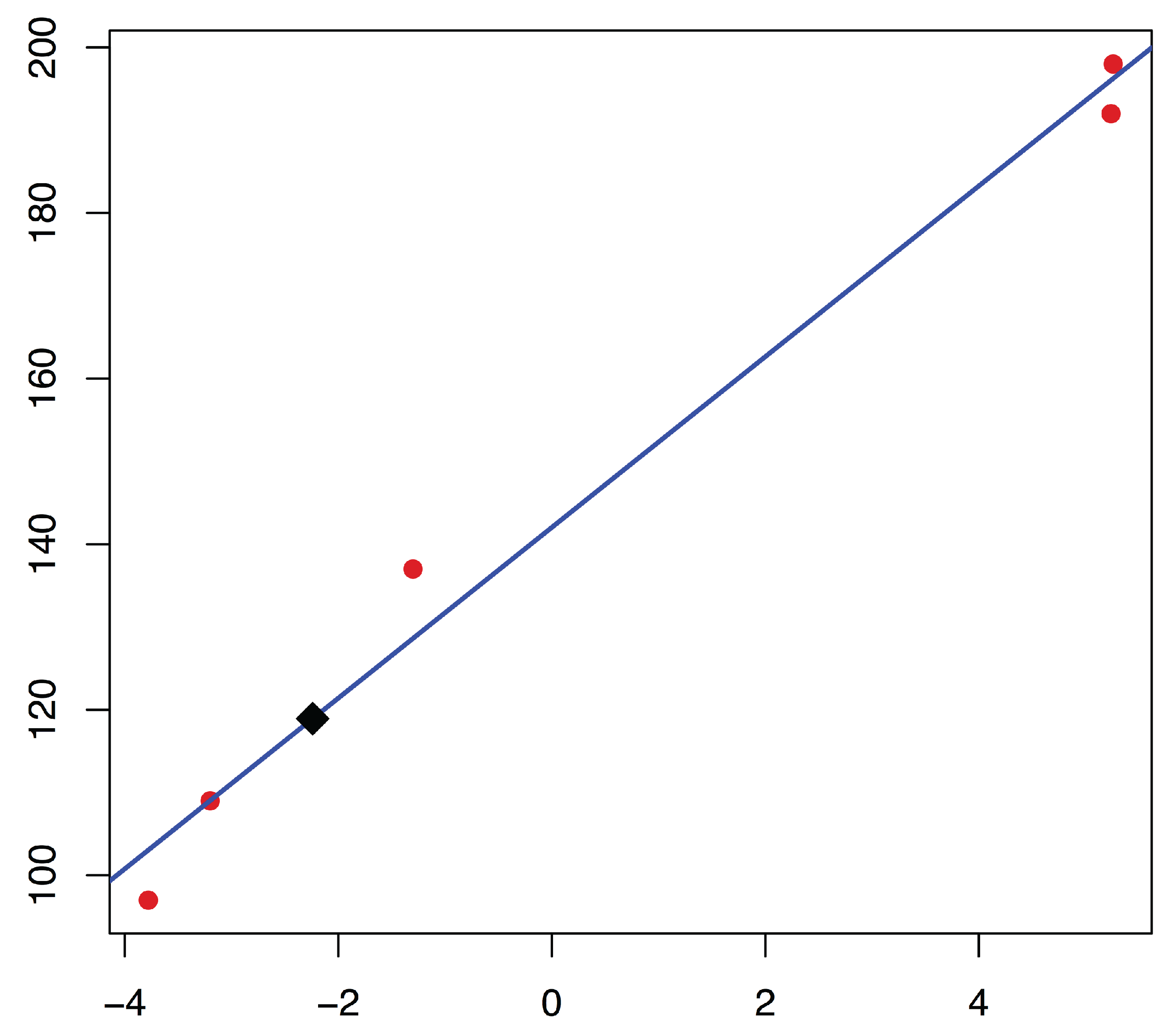
Figure 3.
The regression line in the case study. The black square shows the valuation of the missing option , with score at the horizontal axis.
Figure 3.
The regression line in the case study. The black square shows the valuation of the missing option , with score at the horizontal axis.


Table 1.
Tabular representation of the soft set in Example 1.
| 1 | 0 | 0 | 1 | |
| 1 | 0 | 1 | 0 | |
| 0 | 1 | 0 | 0 |
Table 2.
Tabular representation of the fuzzy soft set in Example 2.
| 0.9 | 0.1 | 0.2 | 0.1 | 0.3 | |
| 0.19 | 0.3 | 0.4 | 0.3 | 0.4 |
Table 3.
Summary of the tabular representations of the three VFSS in Example 2.
| 0.9 | 0.1 | 0.2 | 0.1 | 0.3 | 1.60 | −3 | −1.29 | |
| 0.19 | 0.3 | 0.4 | 0.3 | 0.4 | 1.59 | 3 | 1.29 |
Table 4.
Tabular representation of the partial valuation fuzzy soft set in Section 5. All s are expressed in thousands of euros.
Table 4.
Tabular representation of the partial valuation fuzzy soft set in Section 5. All s are expressed in thousands of euros.
| 137 | ||||||||
| 109 | ||||||||
| 97 | ||||||||
| * | ||||||||
| 192 | ||||||||
| 198 |
Table 5.
Attributes of the comparable six apartments. Source: Real data from the Spanish real estate market (Almería, Spain, 2016).
Table 5.
Attributes of the comparable six apartments. Source: Real data from the Spanish real estate market (Almería, Spain, 2016).
| Item | Surface (sq. m.) | No. of Bathrooms | Quality | No. of Bedrooms |
|---|---|---|---|---|
| 75 | 1 | Normal | 3 | |
| 105 | 2 | Normal | 4 | |
| 75 | 1 | Normal | 2 | |
| 90 | 2 | Normal | 3 | |
| 90 | Normal | 3 | ||
| 105 | 2 | Normal | 3 |
Table 6.
The PVFSS in the real case study in Section 6. Sale prices are given in thousands of euros.
Table 6.
The PVFSS in the real case study in Section 6. Sale prices are given in thousands of euros.
| Item | Surface (sq. m.) | No. of Bathrooms | Quality | No. of Bedrooms | Price |
|---|---|---|---|---|---|
| 95 | |||||
| 1 | 1 | 157 | |||
| 115 | |||||
| 1 | 132 | ||||
| 132 | |||||
| 1 | 157 | ||||
| 1 | * |
Table 7.
Comparison table and scores associated with Table 6. The values have been rounded off.
Table 7.
Comparison table and scores associated with Table 6. The values have been rounded off.
| 0 | 0 | 0 | 0 | 0 | ||||
| 0 | 1 | |||||||
| 0 | 0 | 0 | 0 | 0 | 0 | 0 | ||
| 0 | 0 | 0 | ||||||
| 0 | 0 | 0 | 0 | |||||
| 0 | 0 | |||||||
| 0 |
Table 8.
Possible modalities depending on the type of attribute.
| Quantitative | Qualitative | “Dummy” | |
|---|---|---|---|
| Discrete | Continuous | ||
| 0 | |||
| 1 | |||
| 2 | |||
| ⋮ | ⋮ | ⋮ | ⋮ |
Table 9.
Attributes, modalities and assigned weights.
| Surface | Bathrooms | Quality | Bedrooms | ||||
|---|---|---|---|---|---|---|---|
| Interval | Weight | Number | Weight | Level | Weight | Number | Weight |
| 0.00 | 0 | 0.00 | Bad | 0.04 | 1 | 0.03 | |
| 0.06 | 1 | 0.04 | Low | 0.08 | 2 | 0.06 | |
| 0.08 | 2 | 0.08 | Normal | 0.12 | 3 | 0.09 | |
| 0.10 | 3 | 0.12 | Good | 0.16 | 4 | 0.12 | |
| 0.12 | 4 | 0.16 | Luxury | 0.20 | 5 | 0.14 | |
| 0.14 | 5 | 0.20 | − | − | 6 | 0.16 | |
| 0.16 | − | − | − | − | 7 | 0.17 | |
| 0.18 | − | − | − | − | 8 | 0.18 | |
| 0.20 | − | − | − | − | 9 | 0.19 | |
| 0.22 | − | − | − | − | 10 | 0.20 | |
| 0.24 | − | − | − | − | − | − | |
| 0.26 | − | − | − | − | − | − | |
| 0.28 | − | − | − | − | − | − | |
| 0.30 | − | − | − | − | − | − | |
Table 10.
Weights assigned to all apartments.
| Item | Price | Surface | Bathrooms | Quality | Bedrooms | ||||
|---|---|---|---|---|---|---|---|---|---|
| Value | Weight | Number | Weight | Level | Weight | Number | Weight | ||
| 95,000 | 75 | 0.18 | 1 | 0.04 | Normal | 0.12 | 3 | 0.09 | |
| 157,000 | 105 | 0.24 | 2 | 0.04 | Normal | 0.12 | 4 | 0.12 | |
| 115,000 | 75 | 0.18 | 1 | 0.04 | Normal | 0.12 | 2 | 0.06 | |
| 132,000 | 90 | 0.20 | 2 | 0.08 | Normal | 0.12 | 3 | 0.09 | |
| 132,000 | 90 | 0.20 | 1.5 | 0.06 | Normal | 0.12 | 3 | 0.09 | |
| 157,000 | 105 | 0.24 | 2 | 0.08 | Normal | 0.12 | 3 | 0.09 | |
| * | 114.44 | 0.26 | 1 | 0.04 | Good | 0.16 | 2 | 0.06 | |
© 2017 by the authors. Licensee MDPI, Basel, Switzerland. This article is an open access article distributed under the terms and conditions of the Creative Commons Attribution (CC BY) license (http://creativecommons.org/licenses/by/4.0/).
Share and Cite
MDPI and ACS Style
Alcantud, J.C.R.; Rambaud, S.C.; Torrecillas, M.J.M. Valuation Fuzzy Soft Sets: A Flexible Fuzzy Soft Set Based Decision Making Procedure for the Valuation of Assets. Symmetry 2017, 9, 253. https://doi.org/10.3390/sym9110253
AMA Style
Alcantud JCR, Rambaud SC, Torrecillas MJM. Valuation Fuzzy Soft Sets: A Flexible Fuzzy Soft Set Based Decision Making Procedure for the Valuation of Assets. Symmetry. 2017; 9(11):253. https://doi.org/10.3390/sym9110253
Chicago/Turabian StyleAlcantud, José Carlos R., Salvador Cruz Rambaud, and María J. Muñoz Torrecillas. 2017. "Valuation Fuzzy Soft Sets: A Flexible Fuzzy Soft Set Based Decision Making Procedure for the Valuation of Assets" Symmetry 9, no. 11: 253. https://doi.org/10.3390/sym9110253
Note that from the first issue of 2016, this journal uses article numbers instead of page numbers. See further details here.