Denoising and Feature Extraction Algorithms Using NPE Combined with VMD and Their Applications in Ship-Radiated Noise


School of Marine Science and Technology, Northwestern Polytechnical University, Xi’an 710072, China
*
Authors to whom correspondence should be addressed.
Symmetry 2017, 9(11), 256; https://doi.org/10.3390/sym9110256
Submission received: 10 October 2017
/
Revised: 26 October 2017
/
Accepted: 27 October 2017
/
Published: 1 November 2017
(This article belongs to the Special Issue Information Technology and Its Applications)
Abstract
:A new denoising algorithm and feature extraction algorithm that combine a new kind of permutation entropy (NPE) and variational mode decomposition (VMD) are put forward in this paper. VMD is a new self-adaptive signal processing algorithm, which is more robust to sampling and noise, and also can overcome the problem of mode mixing in empirical mode decomposition (EMD) and ensemble EMD (EEMD). Permutation entropy (PE), as a nonlinear dynamics parameter, is a powerful tool that can describe the complexity of a time series. NPE, a new version of PE, is interpreted as distance to white noise, which shows a reverse trend to PE and has better stability than PE. In this paper, three kinds of ship-radiated noise (SN) signal are decomposed by VMD algorithm, and a series of intrinsic mode functions (IMF) are obtained. The NPEs of all the IMFs are calculated, the noise IMFs are screened out according to the value of NPE, and the process of denoising can be realized by reconstructing the rest of IMFs. Then the reconstructed SN signal is decomposed by VMD algorithm again, and one IMF containing the most dominant information is chosen to represent the original SN signal. Finally, NPE of the chosen IMF is calculated as a new complexity feature, which constitutes the input of the support vector machine (SVM) for pattern recognition of SN. Compared with the existing denoising algorithms and feature extraction algorithms, the effectiveness of proposed algorithms is validated using the numerical simulation signal and the different kinds of SN signal.
1. Introduction
As a part of underwater acoustic signal processing, research on denoising and feature extraction of ship play a very important role in the modern sea battlefield. SN signal contains more characteristic parameters of ship, which is an important indicator of the performance of ship. Therefore, the denoising and feature extraction for SN are critical technologies in the underwater acoustic field [1]. Due to the presence of noise, the physical characteristics of real signal are covered up. That has a great influence on signal analysis, detection, feature extraction, classification and recognition. As the premise of feature extraction, denoising can improve the performance of feature extraction for SN. Research on feature extraction for SN is helpful for the accurate identification of enemy targets, and has significance in theory and practice [2].
Because underwater acoustic signal is non-stationary, non-Gaussian and nonlinear, the traditional signal processing algorithms cannot process it effectively. The Fourier Transform can only show characteristics in the frequency domain; also, the wavelet transform has the limits of the selection of basic functions and decomposition level. As a completely self-adaptive signal processing algorithm, EMD is widely applied not only to fault diagnosis and medical science but also in underwater acoustic signal processing and economics [3]. EMD can decompose the multi-component signal into a series of IMFs based on the local characteristics; nevertheless, EMD has the problems of mode mixing and end effects. To solve the problem of mode mixing, an improved algorithm called EEMD was proposed by Wu et al. in 2009 [4], which can effectively reduce the degree of mode mixing by adding white noise repeatedly. However, both EMD and EEMD lack the foundation of mathematical theory and have the defect of poor robustness [5].
VMD [6], first introduced by Dragomiretskiy et al., is a non-recursive algorithm to analyze non-linear and non-stationary signal, which can adaptively decompose a complex signal into a series of quasi-orthogonal IMFs [7]. Each IMF is compact around a center frequency which can be estimated online. Compared with the EMD and EEMD algorithms, VMD has not only a solid theoretical foundation but also good robustness to noise. It has been applied in the fields of biomedical sciences [8,9], mechanical diagnosis [10] and underwater acoustic signal processing [11]. PE is one of the most effective ways to detect the randomness and dynamic changes of time sequence based on comparison of neighboring values [12,13,14]. However, NPE [15], a new kind of PE, was proposed to classify different sleep stages by Bandt in 2017. NPE is interpreted as distance to white noise, and is regarded as a key parameter that measures depth of sleep. Compared with PE, NPE shows a reverse trend to PE and has better stability for different lengths of time series.
There is a class of denoising algorithms to eliminate noise, which include signal decomposition, screening and reconstruction of components. The basic idea of these algorithms extracts components of signal that was obtained by means of a signal decomposition algorithm and identifies and removes noise components according to the screening principle. Then, the useful components of signal are reconstructed to realize denoising. It is important to select appropriate decomposition algorithm and screening criteria. For example, the denoising algorithm using wavelet analysis has been widely used in different kinds of fields, and achieved good results [16,17]. However, it is limited by the selection of wavelet basis function and the decomposition level [18]. In addition, denoising algorithms based on EMD and its extended algorithms have been extensively studied. In research [19], the high-frequency IMF obtained by EMD is regarded as a noise component, and the rest of the IMFs are reconstructed to achieve denoising. However, this algorithm cannot completely remove noise signal, and lead to the lack of some detailed information. To overcome the shortcomings of these denoising algorithms, some improved denoising algorithms are proposed, which mainly achieve denoising through threshold denoising for IMFs [20,21]. However, the selection of different threshold has a great impact on the result of denoising. These improved denoising algorithms still have some limitations. A new denoising algorithm based on VMD and correlation coefficient is proposed in [22]; it uses the IMFs obtained by VMD to reconstruct the IMFs according to the correlation coefficients between IMFs and original signal to realize denoising. However, the selection of correlation coefficient threshold is a difficult problem.
Recently, many new feature extraction algorithms have been developed and are based on signal decomposition algorithms and measuring complexity in different fields [23,24,25,26]. In research [27], a novel fault feature extraction algorithm for rotating equipment is proposed using improved autoregressive minimum entropy deconvolution and VMD, which is proven to be a more powerful algorithm than the existing ones. In research [28], a feature extraction algorithm for partial discharge is proposed using sample entropy combined with VMD. In the field of underwater acoustic signal processing, PE and multi-scale PE (MPE), as complexity features, are used to extract complexity features of SN combined with EMD and VMD respectively in [11,29]. It has been verified that the two feature extraction algorithms outperform the traditional feature extraction algorithms [30,31].
In this paper, VMD algorithm is used to decompose simulation and real signals, which can accurately decompose signal into IMFs. In addition, NPE has a strong ability for noise recognition. Considering the better performance of VMD and NPE for SN signal, a new denoising algorithm and feature extraction algorithm are presented. The remainder of the paper is organized as follows: in Section 2, the algorithms of VMD, PE, and NPE are described; the review of the denoising and feature extraction algorithm is presented in Section 3; then, the denoising algorithm and feature extraction algorithm are, respectively, applied to SN signal in Section 4 and Section 5; finally, Section 6 concludes this paper.
2. Theory Description
2.1. VMD Algorithm
VMD, as a new signal processing algorithm, is able to adaptively decompose a multi-component signal into multiple numbers of quasi-orthogonal IMFs concurrently. By comparing with EMD and EEMD, VMD has a solid mathematical foundation and defined the IMF as amplitude-modulated-frequency-modulated (AM-FM) signal, like
where and represent time the envelope, and denote the phase and the IMFs. Each IMF has a center frequency and limited bandwidth. In the VMD algorithm, the key decomposition process is the constrained variational problem, which is expressed as
where represent the processed signal, is the number of IMFs, represents convolution. and stand for impulse response and imaginary unit. is the center frequency for each decomposed component, is also the decomposed mono-component. The above constrained variational problem in Equation (2) is addressed by using the penalty factor and the Lagrangian multiplier. The augmented Lagrangian is given by
where and are the Lagrangian multiplier and balancing parameter. The alternating direction multiplier method (ADMM) is applied to obtain the saddle point, then the , and are updated in frequency, like
where and indicate Fourier Transform and time step. The algorithm executes until the convergence stop condition is satisfied. The stop condition is given by
where is the accuracy for convergence. The process of algorithm is depicted in Figure 1. The detail of VMD algorithm and experiment are shown in [6]. In this paper, the decomposition level is the most important parameter, which can be set according to the decomposition level of EMD, and the penalty factor is 2000.
2.2. PE and NPE
PE was described to detect the dynamic changes of time series by comparison with neighboring value of time series. Given a time series with length N, the specific steps of PE are illustrated as follows:
(1) Embedded dimension m of the time series with a time delay is constructed as follows:
where is .
(2) Each vector of is rearranged in ascending order as
If , then .
(3) Therefore, for time series , each vector of can be obtained as
where , . There are different symbol series, and only indicates one symbol series.
(4) The probability of each symbol series is calculated as , the PE of time series can be defined according to the form of Shannon entropy as
(5) When , reaches the maximum . Consequently, the PE can be standardized as
It is obvious that the value of is from 0 to 1. The details of PE method are shown in [12].
NPE, a new version of PE, is interpreted as distance to white noise. The steps of NPE is same with PE from step (1) to step (3). In step (4), the NPE of time series can be defined as
in the Formula (10), is replaced by , and a constant is added. When , reaches the smallest value 0, this means that the distance to white noise is 0.
In order to prove the stability of NPE with different data lengths, simulation experiments of sinusoidal signal with different frequencies are carried out. The simulation signal is , represents frequency and sampling frequency is Hz. For PE and NPE, the parameters of time delay and the embedded dimension are set as one and three respectively. Table 1 and Table 2 show the PEs and NPEs of simulation signal with different frequencies and lengths, respectively. As it can be seen in Table 1 and Table 2, NPE is more stable than PE for simulation signal with different frequencies and lengths.
2.3. Analysis of the Simulation Signal Using VMD and NPE
In order to verify the effectiveness of the new algorithm, simulation experiments are carried out. The simulation signals are given by
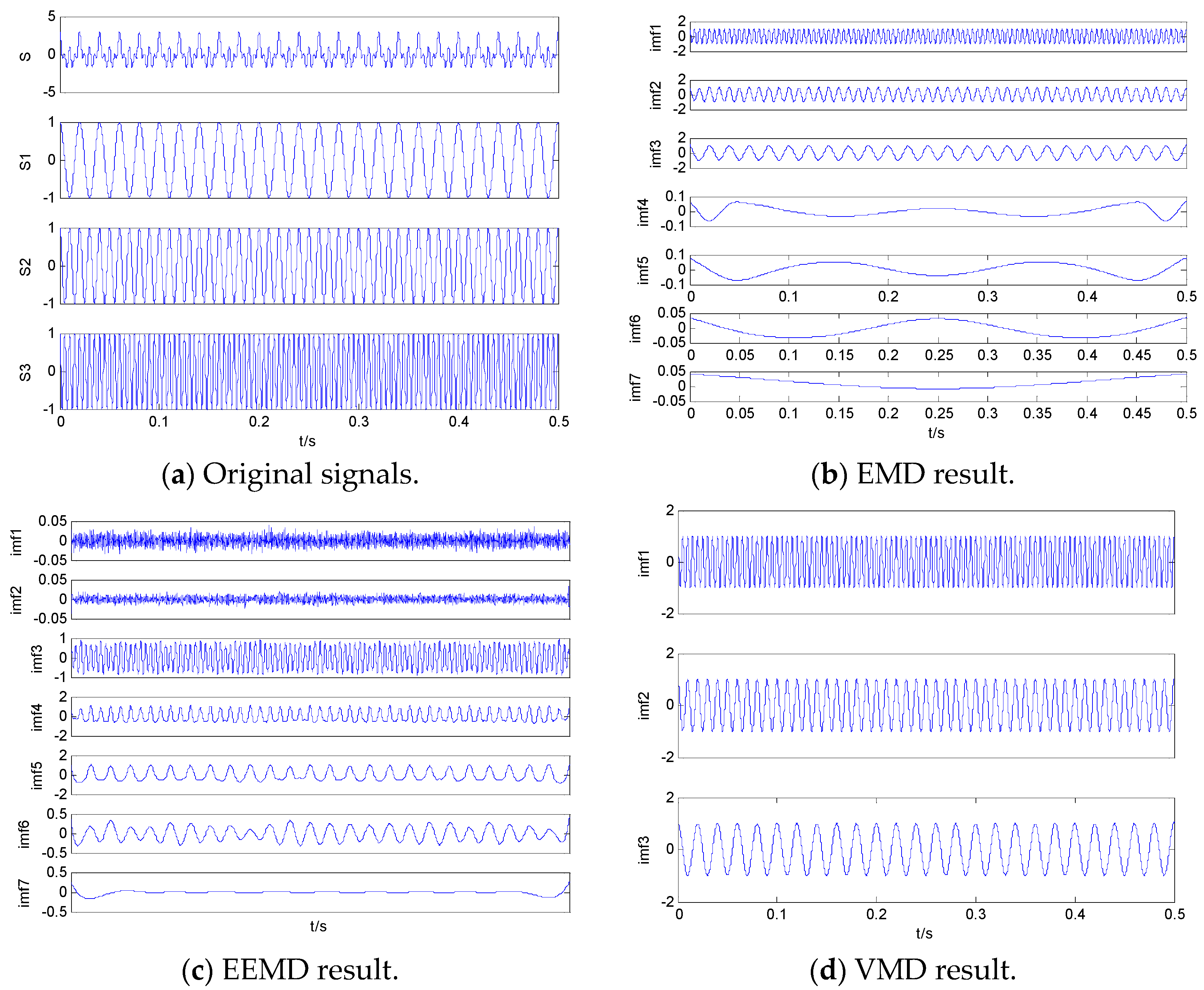
where , and are the three components of , sampling frequency is Hz. The parameters of time delay and the embedded dimension are also one and three respectively. Three algorithms are used to decompose . The original signals and the decomposition results are shown in Figure 2. For EEMD, the white noise standard deviation and the number of white noise are set as 0.3 and 100. As it can be seen in Figure 2, VMD shows the best performance when the decomposition level is 3, the IMFs by VMD are more similar to the original signals. Also, Table 3 and Table 4 show the PEs and NPEs of IMFs by three different decomposition algorithms. As it can be seen in Table 3 and Table 4, the NPEs of IMFs by VMD are closer to real values than other NPEs and PEs of IMFs. Therefore, the proposed algorithm can well reflect the features of the original signal, which is very beneficial to feature extraction.
3. Denoising and Feature Extraction Algorithms Using VMD and NPE
3.1. Denoising Algorithm
In view of the advantages of NPE and VMD, a new denoising algorithm can be designed. The main steps are as follows:
- Step 1
- Decompose signal by EMD.
- Step 2
- Select the decomposition level of VMD according to the decomposition level of EMD.
- Step 3
- Decompose signal by VMD, IMFs can be obtained.
- Step 4
- Calculate the NPE of each IMF.
- Step 5
- Screen out the noise IMFs according to the value of NPE. Normally when NPE of IMF is less than 0.1, it is regarded as the noise IMF.
- Step 6
- Reconstruct the useful IMFs with NPE greater than 0.1. After the reconstruction, the process of denoising is completed.
3.2. Feature Extraction Algorithm
VMD has many applications in feature extraction, the effectiveness of the algorithm is illustrated in many researches. However, NPE as a new PE is only used in the field of medicine. A new feature extraction algorithm combining VMD and NPE can be designed.
The main steps are as follows:
- Step 1
- Decompose the reconstructed signal by EMD.
- Step 2
- Select the decomposition level of VMD according to the decomposition level of EMD.
- Step 3
- Decompose the reconstructed signal by VMD, IMFs can be obtained.
- Step 4
- Calculate the energy intensity of each IMF.
- Step 5
- Select the principal IMF, namely PIMF. Normally PIMF is the IMF with the maximum energy intensity.
- Step 6
- Calculate the NPEs of PIMFs.
- Step 7
- Put the NPEs of PIMFs into SVM, the classification results can reflect the effectiveness of the feature extraction algorithm.
4. Denoising of Simulation Signal
To prove the validity of the denoising algorithm, two simulation experiments are carried out. Moreover, the proposed denoising algorithm is compared with the existing algorithms.
4.1. Simulation Experiment 1
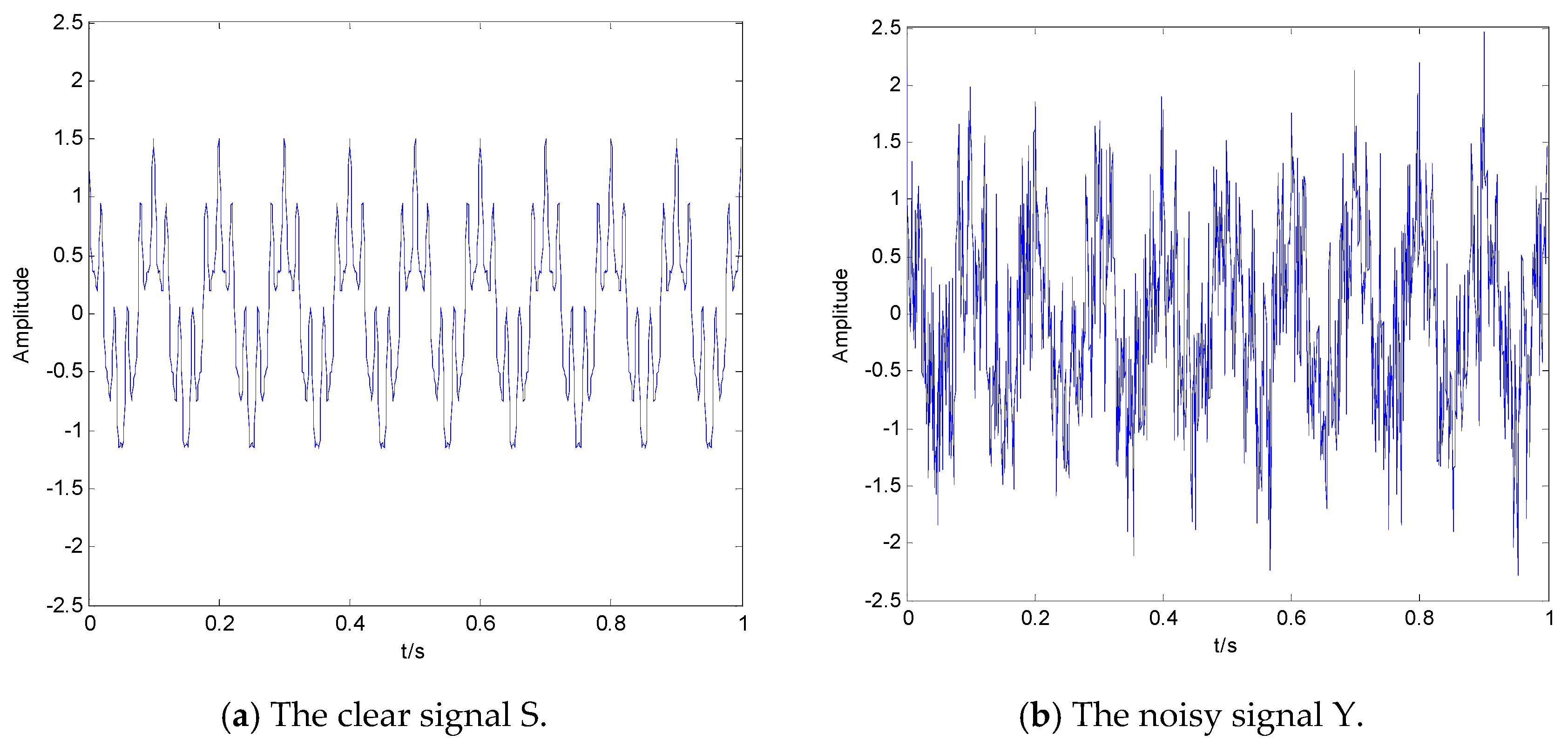
The clear signal is composed of , and , and the noisy signal has two components: and . The simulation signals are listed as follows:
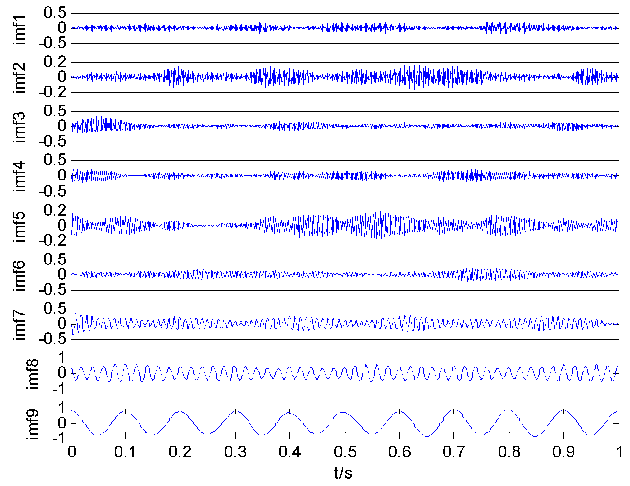
where , and represent the three sinusoidal signals of different frequencies. is 0.5 times the standard Gaussian white noise. The sampling frequency is 1 kHz, and data length is 1000. The clear signal and the noisy signal are shown in Figure 3, and the decomposition result of signal by VMD is shown in Figure 4. The decomposition level of VMD is the same with EMD.
As shown in Figure 4, it can easily be seen that S1, S2 and S3 correspond to IMF9, IMF8 and IMF7, which are the useful IMFs. Table 5, Table 6 and Table 7 are listed the correlation coefficients (CC) between each IMF and Y, and PE and NPE of Each of IMF. For PE and NPE, the parameters of time delay and the embedded dimension are one and three respectively.
As shown in Table 5, Table 6 and Table 7, the proposed denoising algorithm using VMD and NPE is easier to recognize the noise IMFs, because NPE of the useful IMF is one magnitude order higher compared with NPE of the noise IMF. It is difficult to confirm the thresholds of CC and PE. When the thresholds of CC, PE and NPE are set as 0.2, 0.9 and 0.1, the denoising results are shown in Figure 5. Furthermore, the SNRs and root mean square errors (RMSE) of the noisy signal and the denoising results are listed in Table 8. For wavelet (WT) denoising, soft threshold method is used to quantify the wavelet coefficient, WT basis function and decomposition levels are db4 and 3, respectively. To summarize, it can be seen that the proposed denoising algorithm has better denoising performance and overcomes the problem of threshold selection.
4.2. Simulation Experiment 2
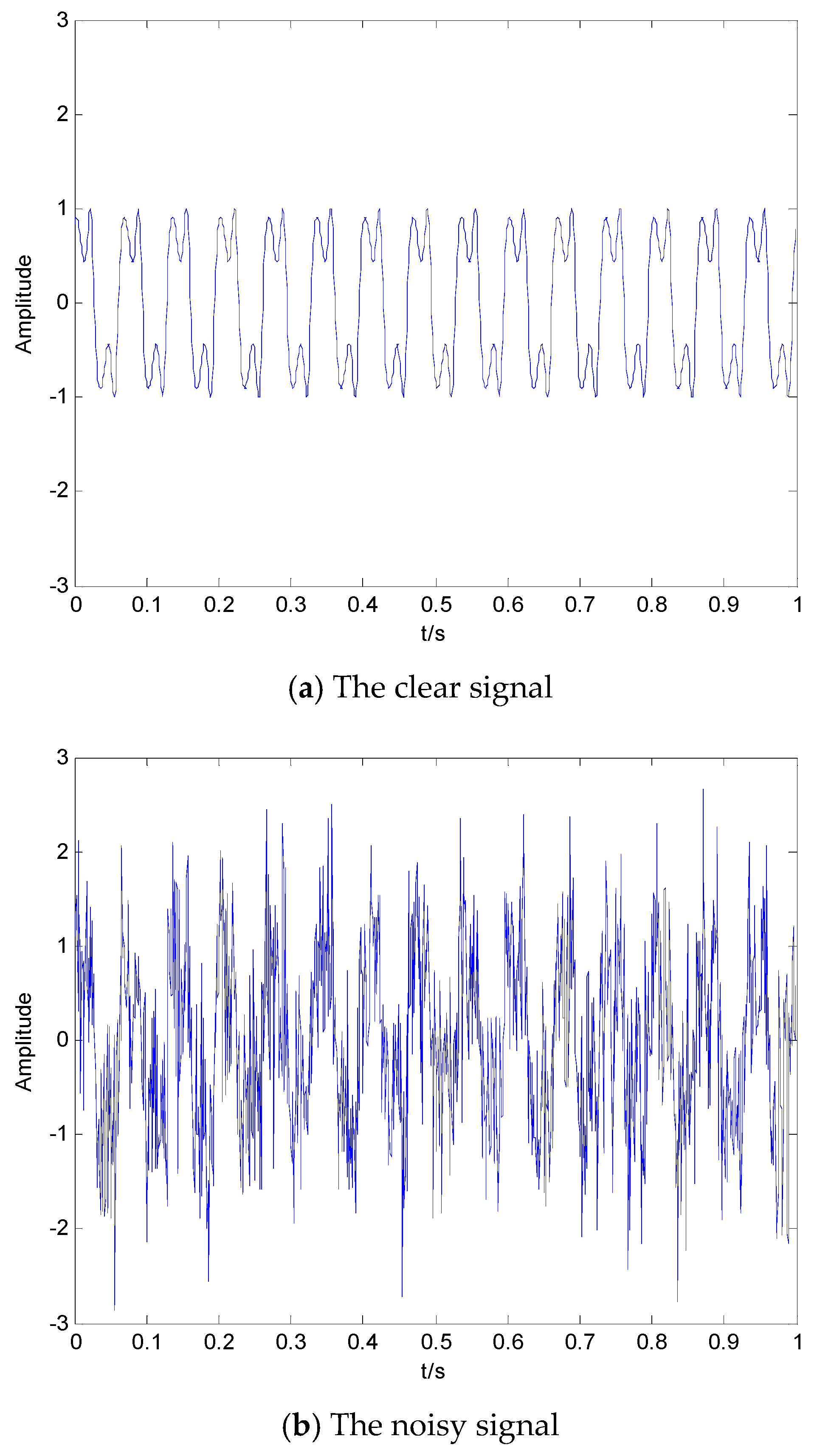
In research [32], the convex 1-D 2-order total variation denoising algorithm for vibration signal is proposed. In order to validate the effectiveness of the proposed denoising algorithm in this paper, the same simulation experiments are carried out. The simulation signals are as follows:
where is a modulating signal shown in Figure 6a. The noisy signal is composed of S and Gaussian white noise with mean 0 and variance 0.5 shown in Figure 6b.
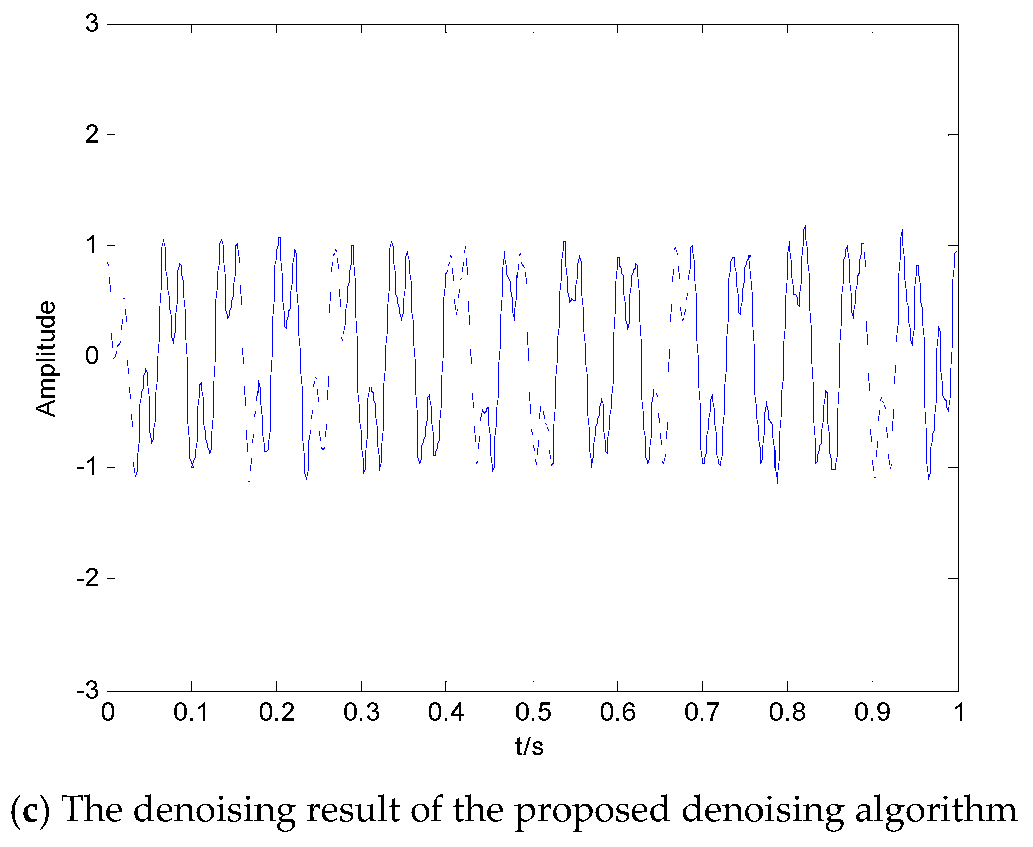
The result of the proposed denoising algorithm is shown in Figure 6c. In addition, the results of SNRs for different variances of Gaussian white noise and different denoising algorithms are shown in Table 9. The results of the other three denoising algorithms can be seen in [32]. As shown in Table 9, the proposed denoising algorithm has high SNRs for different variances of Gaussian white noise.
5. Feature Extraction of SN
5.1. The Denoising of SN
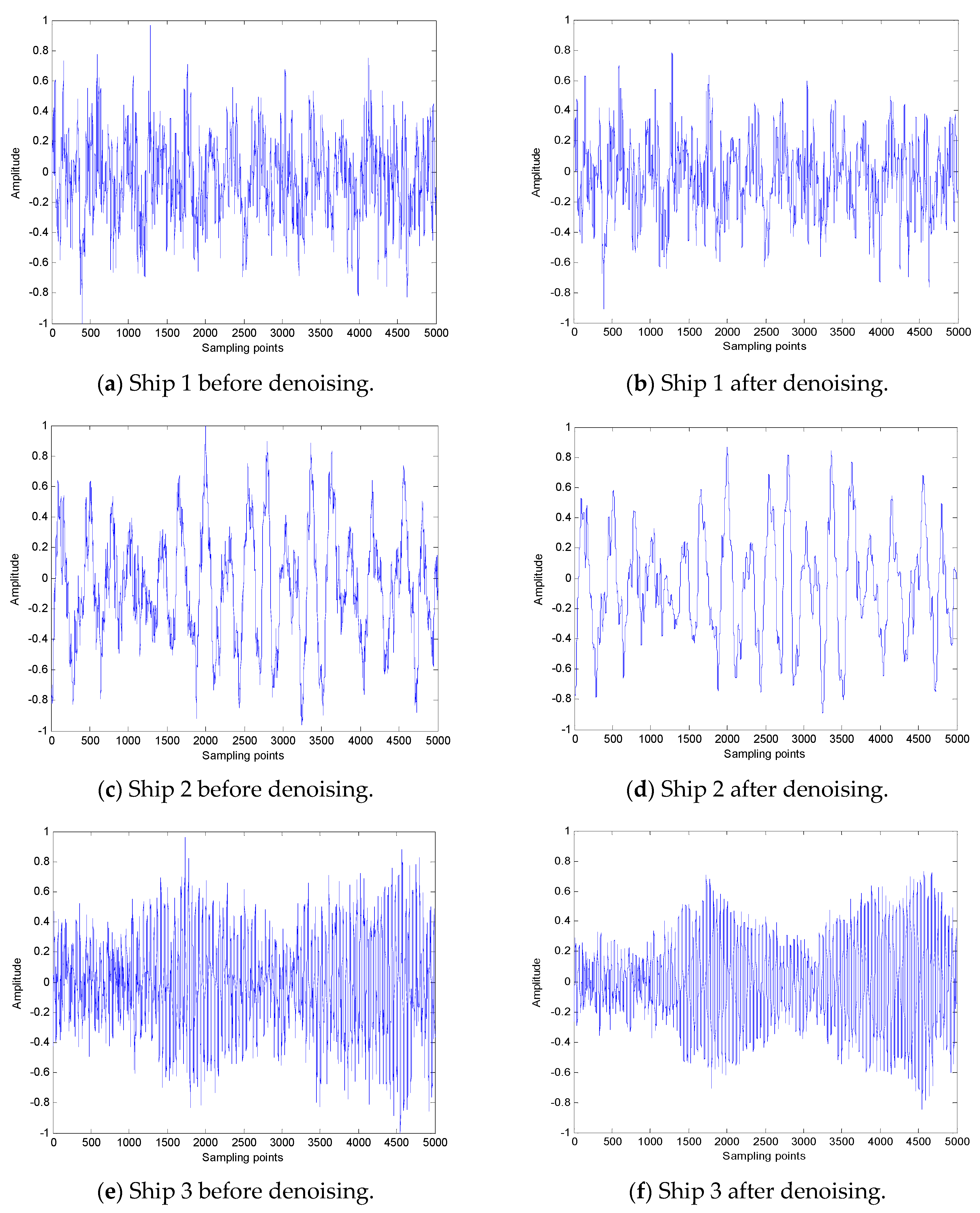
The proposed denoising algorithm is applied to three kinds of SN. The same SN signals are used in this paper and [11]; the details of SN signals can be found in [11]. The sampling frequency and sampling points of three kinds of SN are set as 44.1 kHz and 5000, respectively. Each sample is normalized to get the three kinds of normalized SN signal, namely, ship 1, ship 2 and ship 3, as shown in Figure 7. The denoising results of three kinds of SN are also shown in Figure 7 [12].
5.2. The VMD of SN
For comparison purposes, the decomposition level of VMD is set to 8 for three kinds of SN after denoising according to the results of EMD. The results of VMD for three kinds of SN are shown in Figure 8. As shown in Figure 8, 8 IMFs of each ship are listed in descending order by frequency. In this paper, PIMF is the IMF with the most energy intensity, which has the same definition in [11,29]. The distribution of PIMF for three kinds of SN is listed in Table 10.
5.3. Feature Extraction of SN
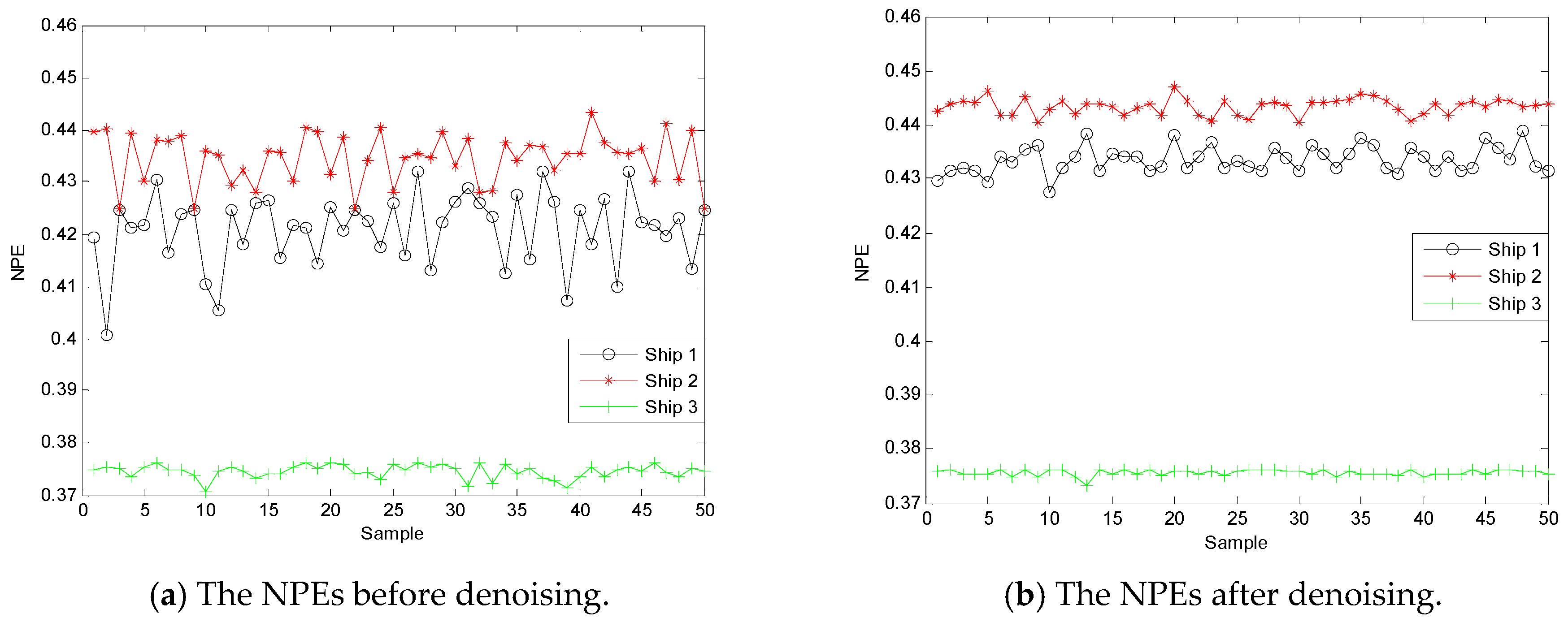
In research [11], feature extraction algorithm of SN has been proven to be more efficient than traditional feature extraction algorithms, which extracts the features of SN using VMD and MPE. In order to prove the validity of the proposed feature extraction algorithm, the NPEs of PIMFs are calculated by comparing with the PEs of PIMF (when the scale of MPE is 1 in [11]). Figure 9a and Figure 10a are the PE and NPE distributions of PIMF before denoising, and Figure 9b and Figure 10b are the distributions after denoising (50 samples for each ship). As shown in Figure 9 and Figure 10, ship 3 can be easily identified using all the algorithms, the features of some samples for ship 2 and ship 3 are close.
5.4. Classification of SN
The features of PEs and NPEs are put into SVM, the classification results can reflect the effectiveness of the proposed denoising algorithm and the feature extraction algorithm. Table 11 and Table 12 are the PE and NPE classification results before denoising, and Table 13 and Table 14 are the classification results after denoising. As shown in Table 11, Table 12, Table 13 and Table 14, the recognition rates of PEs and NPEs after denoising are higher than ones before denoising. In addition, the recognition rates of NPEs are higher than ones of PEs, whether before or after denoising.
6. Conclusions
VMD as a new self-adaptive signal processing algorithm is more robust to sampling and noise, and also can overcome the problem of mode mixing in EMD and EEMD. NPE as a new version of PE is interpreted as distance to white noise, which shows a reverse trend to PE and has better stability than PE. Considering the better performance of VMD and NPE, a new denoising algorithm and feature extraction algorithm are presented. The proposed algorithms mainly have the following advantages:
- (1)
- NPE, a new kind of PE, is firstly applied to denoising and feature extraction of SN combined with VMD.
- (2)
- The simulation results show that the proposed denoising algorithm has better denoising performance than the existing algorithms and overcomes the problem of threshold selection.
- (3)
- The proposed denoising algorithm is used to denoise SN signal; it concluded that the features of PE and NPE after denoising are beneficial to classification and recognition for SN signal.
- (4)
- The proposed feature extraction algorithm is used to extract the feature of SN signal, the experimental results show that the feature of NPE has a higher recognition rate than that of PE in [11].
In further studies, the two algorithms will be greatly improved by achieving better denoising and feature extraction performances.
Acknowledgments
Authors gratefully acknowledge the supported by National Natural Science Foundation of China (No. 51179157, No. 51409214, No. 11574250 and No. 51709228).
Author Contributions
Yuxing Li contributed the new algorithm, all authors designed and analyzed the experiments, Yuxing Li performed the experiments and wrote this article.
Conflicts of Interest
The authors declare no conflict of interest.
References
- Siddagangaiah, S.; Li, Y.; Guo, X.; Chen, X.; Zhang, Q.; Yang, K.; Yang, Y. A Complexity-Based Approach for the Detection of Weak Signals in Ocean Ambient Noise. Entropy 2016, 18, 101. [Google Scholar] [CrossRef]
- Wang, S.G.; Zeng, X.Y. Robust underwater noise targets classification using auditory inspired time-frequency analysis. Appl. Acoust. 2014, 78, 68–76. [Google Scholar] [CrossRef]
- Huang, N.E.; Shen, Z.; Long, S.R.; Wu, M.C.; Shih, H.H.; Zheng, Q.A.; Yen, N.; Tung, C.C.; Liu, H.H. The empirical mode decomposition and the Hilbert spectrum for nonlinear and non-stationary time series analysis. Proc. R. Soc. Lond. 1998, 454, 903–995. [Google Scholar] [CrossRef]
- Wu, Z.; Huang, N.E. Ensemble empirical mode decomposition: A noise-assisted data analysis method. Adv. Adapt. Data Anal. 2009, 1, 1–41. [Google Scholar] [CrossRef]
- Wang, Y.; Marker, R. Filter bank property of variational mode decomposition and its applications. Signal Process. 2016, 120, 509–521. [Google Scholar] [CrossRef]
- Dragomiretskiy, K.; Zosso, D. Variational mode decomposition. IEEE Trans. Signal Process. 2014, 62, 531–544. [Google Scholar] [CrossRef]
- Wang, Y.X.; Liu, F.Y.; Jiang, Z.S.; He, S.L.; Mo, Q.Y. Complex variational mode decomposition for signal processing applications. Mech. Syst. Signal Process. 2017, 86, 75–85. [Google Scholar] [CrossRef]
- Ping, X.; Yang, F.M.; Li, X.X.; Yong, Y.; Chen, X.L.; Zhang, L.T. Functional coupling analyses of electroencephalogram and electromyogram based on variational mode decomposition-transfer entropy. Acta Phys. Sin. 2016, 65, 118701. [Google Scholar]
- Tripathy, R.K.; Sharma, L.N.; Dandapat, S. Detection of shockable ventricular arrhythmia using variational mode decomposition. J. Med. Syst. 2016, 40, 1–13. [Google Scholar] [CrossRef] [PubMed]
- Wang, Y.X.; Markert, R.; Xiang, J.W.; Zheng, W.G. Research on variational mode decomposition and its application in detecting rub-impact fault of the rotor system. Mech. Syst. Signal Process. 2015, 60–61, 243–251. [Google Scholar] [CrossRef]
- Li, Y.; Li, Y.; Chen, X.; Yu, J. A Novel Feature Extraction Method for Ship-Radiated Noise Based on Variational Mode Decomposition and Multi-Scale Permutation Entropy. Entropy 2017, 19, 342. [Google Scholar]
- Bandt, C.; Pompe, B. Permutation entropy: A natural complexity measure for time series. Phys. Rev. Lett. 2002, 88, 174102. [Google Scholar] [CrossRef] [PubMed]
- Zanin, M.; Zunino, L.; Rosso, O.A.; Papo, D. Permutation Entropy and Its Main Biomedical and Econophysics Applications: A Review. Entropy 2012, 14, 1553–1577. [Google Scholar] [CrossRef]
- Keller, K.; Mangold, T.; Stolz, I.; Werner, J. Permutation Entropy: New Ideas and Challenges. Entropy 2017, 19, 134. [Google Scholar] [CrossRef]
- Lei, Y.; He, Z.; Zi, Y. Application of the EEMD method to rotor fault diagnosis of rotating machinery. Mech. Syst. Signal Process. 2009, 23, 1327–1338. [Google Scholar] [CrossRef]
- Murguia, J.S.; Campos, C.E. Wavelet analysis of chaotic time series. Revista Mexicana De Fisica 2006, 52, 155–162. [Google Scholar]
- Liu, Y.X.; Yang, G.S.; Jia, Q. Adaptive Noise Reduction for Chaotic Signals Based on Dual-Lifting Wavelet Transform. Acta Electron. Sin. 2011, 39, 13–17. [Google Scholar]
- Zhang, L.; Bao, P.; Wu, X. Multiscale LMMSE-based image denoising with optimal wavelet selection. IEEE Trans. Circ. Syst. Video Technol. 2005, 15, 469–481. [Google Scholar] [CrossRef]
- Boudraa, A.O.; Cexus, J.C. EMD-Based Signal Filtering. IEEE Trans. Instrum. Meas. 2007, 56, 2196–2202. [Google Scholar] [CrossRef]
- Omitaomu, O.A.; Protopopescu, V.A.; Ganguly, A.R. Empirical Mode Decomposition Technique with Conditional Mutual Information for Denoising Operational Sensor Data. IEEE Sens. J. 2011, 11, 2565–2575. [Google Scholar] [CrossRef]
- Kopsinis, Y.; Mclaughlin, S. Development of EMD-Based Denoising Methods Inspired by Wavelet Thresholding. IEEE Trans. Signal Process. 2009, 57, 1351–1362. [Google Scholar] [CrossRef]
- Liu, J.; Lv, Y. Fault Diagnosis for Rolling Bearing Based on the Variational Mode Decomposition De-Noising. Mach. Des. Manuf. 2015, 10, 21–25. [Google Scholar]
- Li, X.; Li, C. Pretreatment and Wavelength Selection Method for Near-Infrared Spectra Signal Based on Improved CEEMDAN Energy Entropy and Permutation Entropy. Entropy 2017, 19, 380. [Google Scholar] [CrossRef]
- Deng, W.; Zhao, H.; Yang, X.; Dong, C. A Fault Feature Extraction Method for Motor Bearing and Transmission Analysis. Symmetry 2017, 9, 60. [Google Scholar] [CrossRef]
- Yi, C.; Lv, Y.; Ge, M.; Xiao, H.; Yu, X. Tensor Singular Spectrum Decomposition Algorithm Based on Permutation Entropy for Rolling Bearing Fault Diagnosis. Entropy 2017, 19, 139. [Google Scholar] [CrossRef]
- Gao, Y.; Villecco, F.; Li, M.; Song, W. Multi-Scale permutation entropy based on improved LMD and HMM for rolling bearing diagnosis. Entropy 2017, 19, 176. [Google Scholar] [CrossRef]
- Li, Q.; Ji, X.; Liang, S.Y. Incipient Fault Feature Extraction for Rotating Machinery Based on Improved AR-Minimum Entropy Deconvolution Combined with Variational Mode Decomposition Approach. Entropy 2017, 19, 317. [Google Scholar] [CrossRef]
- Shang, H.; Lo, K.L.; Li, F. Partial Discharge Feature Extraction Based on Ensemble Empirical Mode Decomposition and Sample Entropy. Entropy 2017, 19, 439. [Google Scholar] [CrossRef]
- Li, Y.X.; Li, Y.A.; Chen, Z.; Chen, X. Feature extraction of ship-radiated noise based on permutation entropy of the intrinsic mode function with the highest energy. Entropy 2016, 18, 393. [Google Scholar] [CrossRef]
- Yang, H.; Li, Y.; Li, G. Energy analysis of ship-radiated noise based on ensemble empirical mode decomposition. J. Shock Vib. 2015, 34, 55–59. [Google Scholar]
- Li, Y.; Li, Y.; Chen, X. Ships’ radiated noise feature extraction based on EEMD. J. Shock Vib. 2017, 36, 114–119. [Google Scholar]
- Yi, C.; Lv, Y.; Dang, Z.; Xiao, H. A Novel Mechanical Fault Diagnosis Scheme Based on the Convex 1-D Second-Order Total Variation Denoising Algorithm. Appl. Sci. 2016, 6, 403. [Google Scholar] [CrossRef]
Figure 1.
The flowchart of VMD algorithm.
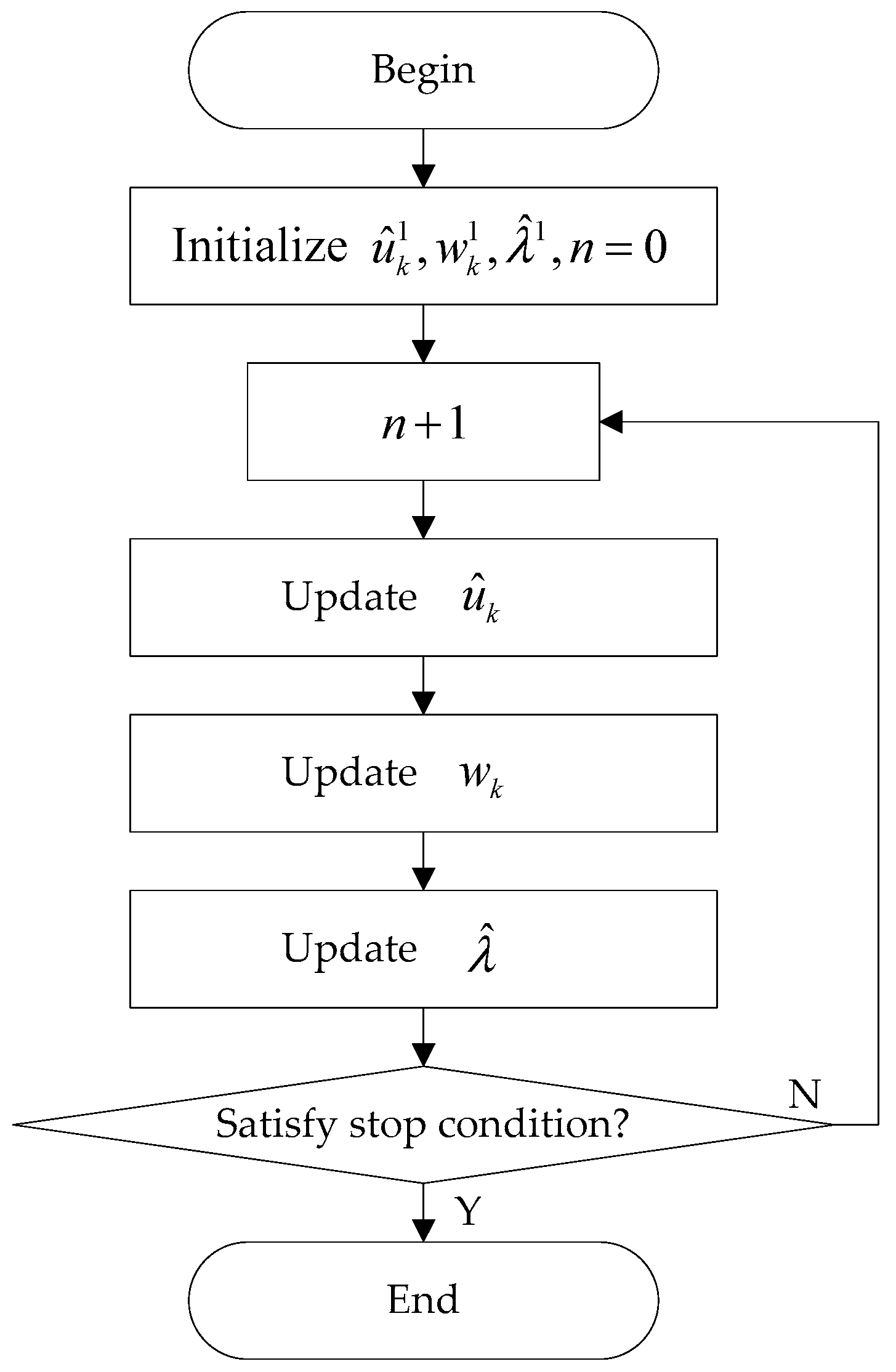
Figure 2.
The simulation signals and the decomposition result of EMD, EEMD and VMD. (a) Original signals; (b) EMD result; (c) EEMD result; (d) VMD result.
Figure 2.
The simulation signals and the decomposition result of EMD, EEMD and VMD. (a) Original signals; (b) EMD result; (c) EEMD result; (d) VMD result.

Figure 3.
The (a) clear signal and (b) the noisy signal .

Figure 4.
The decomposition result of signal Y by VMD.

Figure 5.
The denoising results of different algorithms. (a) Denoising using VMD and CC; (b) Denoising using VMD and PE; (c) Denoising using VMD and NPE; (d) Denoising using WT.
Figure 5.
The denoising results of different algorithms. (a) Denoising using VMD and CC; (b) Denoising using VMD and PE; (c) Denoising using VMD and NPE; (d) Denoising using WT.
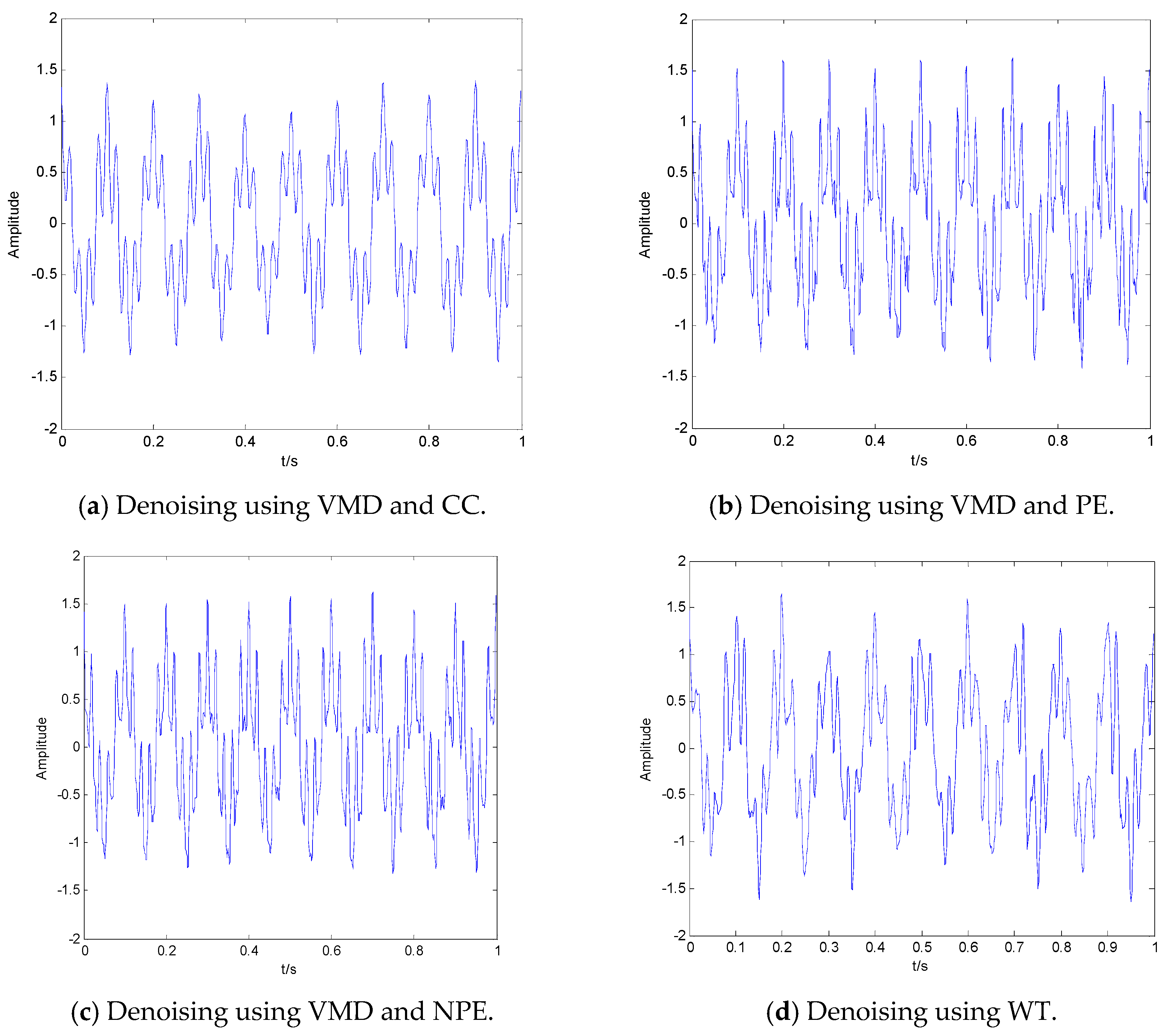
Figure 6.
The clear signal, noisy signal and denoising result. (a) The clear signal; (b) The noisy signal; (c) The denoising result of the proposed denoising algorithm.
Figure 6.
The clear signal, noisy signal and denoising result. (a) The clear signal; (b) The noisy signal; (c) The denoising result of the proposed denoising algorithm.


Figure 7.
The three kinds of SN before and after denoising. (a) Ship 1 before denoising; (b) Ship 1 after denoising; (c) Ship 2 before denoising; (d) Ship 2 after denoising; (e) Ship 3 before denoising; (f) Ship 3 after denoising.
Figure 7.
The three kinds of SN before and after denoising. (a) Ship 1 before denoising; (b) Ship 1 after denoising; (c) Ship 2 before denoising; (d) Ship 2 after denoising; (e) Ship 3 before denoising; (f) Ship 3 after denoising.

Figure 8.
The results of VMD for three kinds of SN. (a) Ship 1; (b) Ship 2; (c) Ship 3.
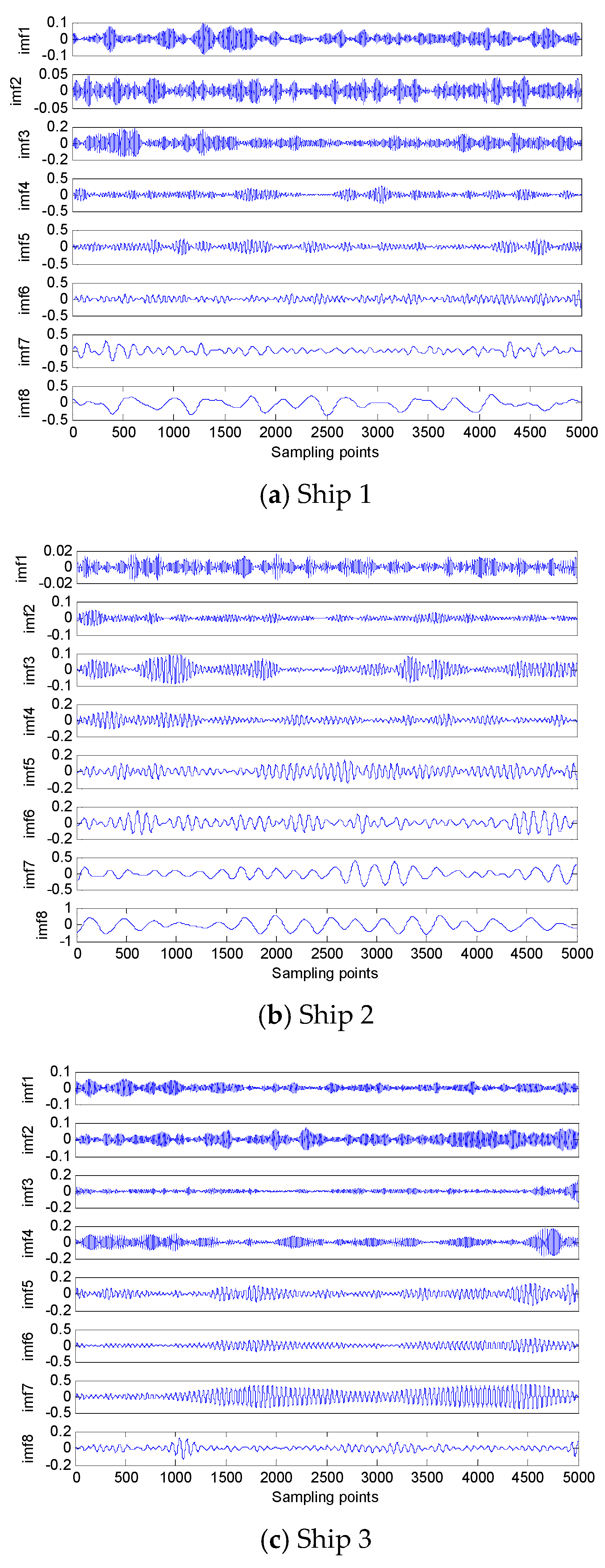
Figure 9.
The PEs distribution of PIMFs before and after denoising. (a) The PEs before denoising; (b) The PEs after denoising.
Figure 9.
The PEs distribution of PIMFs before and after denoising. (a) The PEs before denoising; (b) The PEs after denoising.
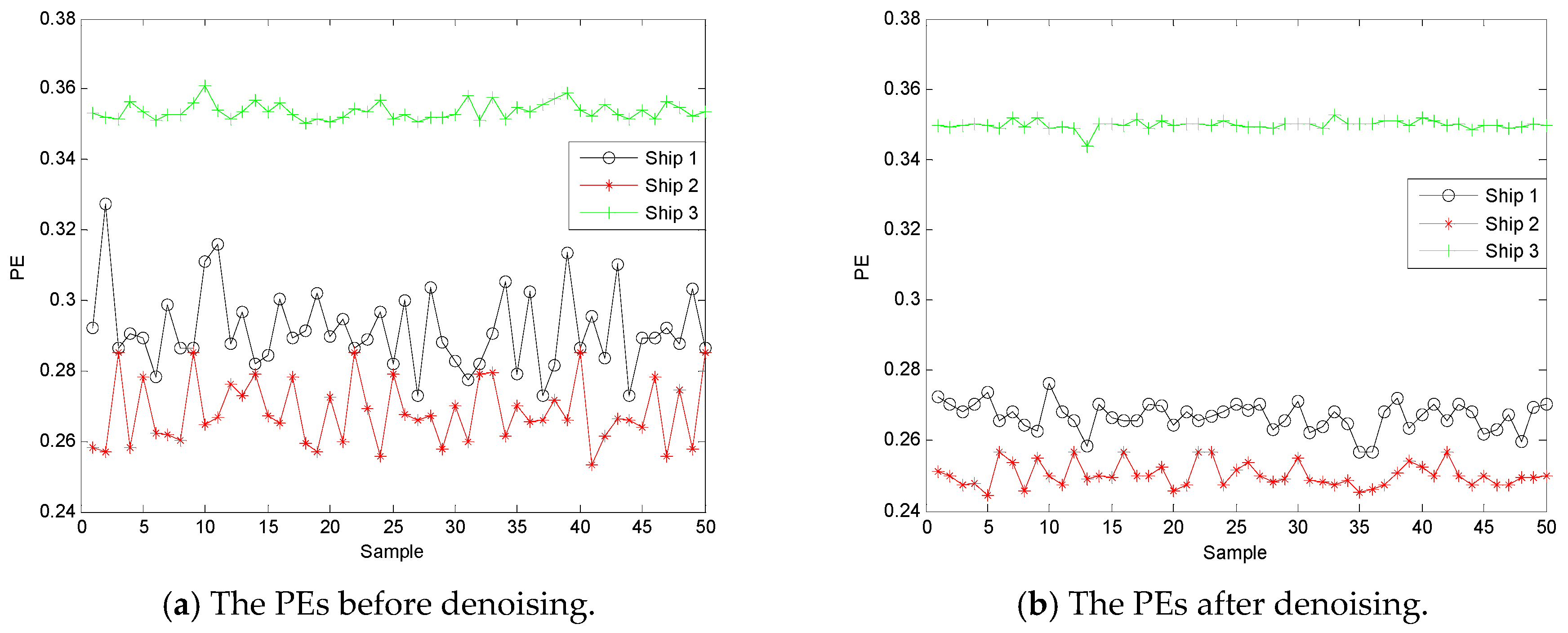
Figure 10.
The NPEs distribution of PIMFs before and after denoising. (a) The NPEs before denoising; (b) The NPEs after denoising.
Figure 10.
The NPEs distribution of PIMFs before and after denoising. (a) The NPEs before denoising; (b) The NPEs after denoising.


Table 1.
The PEs of different frequencies and data lengths.
| Data Length | 100 Hz | 200 Hz | 500 Hz | 1000 Hz |
|---|---|---|---|---|
| 1000 | 0.445 | 0.4869 | 0.5937 | 0.7154 |
| 2000 | 0.4447 | 0.4866 | 0.5929 | 0.7139 |
| 3000 | 0.449 | 0.496 | 0.5834 | 0.6915 |
Table 2.
The NPEs of different frequencies and data lengths.
| Data Length | 100 Hz | 200 Hz | 500 Hz | 1000 Hz |
|---|---|---|---|---|
| 1000 | 0.3137 | 0.2948 | 0.2418 | 0.1678 |
| 2000 | 0.3137 | 0.2948 | 0.2419 | 0.1681 |
| 3000 | 0.3136 | 0.2945 | 0.2426 | 0.171 |
Table 3.
The PEs of IMFs.
| Signal | PE | EMD | EEMD | VMD | |||
|---|---|---|---|---|---|---|---|
| S1 | 0.4213 | IMF3 | 0.4217 | IMF5 | 0.4291 | IMF3 | 0.4195 |
| S2 | 0.4483 | IMF2 | 0.449 | IMF4 | 0.4816 | IMF2 | 0.4469 |
| S3 | 0.4946 | IMF1 | 0.4962 | IMF3 | 0.4963 | IMF1 | 0.4936 |
Table 4.
The NPEs of IMFs.
| Signal | NPE | EMD | EEMD | VMD | |||
|---|---|---|---|---|---|---|---|
| S1 | 0.3235 | IMF3 | 0.3235 | IMF5 | 0.321 | IMF3 | 0.3235 |
| S2 | 0.3137 | IMF2 | 0.3137 | IMF4 | 0.3007 | IMF2 | 0.3137 |
| S3 | 0.2947 | IMF1 | 0.2944 | IMF3 | 0.2944 | IMF1 | 0.2946 |
Table 5.
The CCs between IMFs and Y.
| Parameter | IMF1 | IMF2 | IMF3 | IMF4 | IMF5 | IMF6 | IMF7 | IMF8 | IMF9 |
|---|---|---|---|---|---|---|---|---|---|
| CC | 0.1643 | 0.1425 | 0.1567 | 0.1633 | 0.147 | 0.1607 | 0.196 | 0.4075 | 0.6919 |
Table 6.
The PEs of IMFs.
| Parameter | IMF1 | IMF2 | IMF3 | IMF4 | IMF5 | IMF6 | IMF7 | IMF8 | IMF9 |
|---|---|---|---|---|---|---|---|---|---|
| PE | 0.9296 | 0.9909 | 0.999 | 0.9764 | 0.9466 | 0.8782 | 0.7427 | 0.6054 | 0.4463 |
Table 7.
The NPEs of IMFs.
| Parameter | IMF1 | IMF2 | IMF3 | IMF4 | IMF5 | IMF6 | IMF7 | IMF8 | IMF9 |
|---|---|---|---|---|---|---|---|---|---|
| NPE | 0.0458 | 0.0088 | 0.0017 | 0.0084 | 0.0383 | 0.0688 | 0.1642 | 0.2416 | 0.3146 |
Table 8.
The result of SNRs for different algorithms.
| Parameter | Y | CC | PE | NPE | WT |
|---|---|---|---|---|---|
| SNR (db) | 2.7178 | 12.0307 | 14.7721 | 15.5929 | 8.3378 |
| RMSE | 0.56 | 0.1448 | 0.1453 | 0.1434 | 0.1671 |
Table 9.
The SNRs for different denoising algorithms.
| Denoising Algorithms | The Variance of Gaussian White Noise | ||
|---|---|---|---|
| 0.4 | 0.5 | 0.6 | |
| The Proposed Denoising Algorithm (db) | 12.58 | 11.69 | 11.25 |
| The Convex 1-D 2-Order Total Variation Algorithm (db) | 12.13 | 11.31 | 10.28 |
| The Convex 1-D 1-Order Total Variation Algorithm (db) | 4.69 | 3.31 | 2.17 |
| Wavelet Denoising Algorithm (db) | 10.28 | 9.20 | 8.31 |
| The noisy signal (db) | 0.9778 | –0.0494 | –0.8239 |
Table 10.
The distribution of PIMF for three kinds of SN.
| Level | Ship 1 | Ship 2 | Ship 3 |
|---|---|---|---|
| The level of PIMF | 8 | 8 | 7 |
Table 11.
The PE classification results before denoising.
| Ship | Train | Test | Overall Correctness (%) | ||
|---|---|---|---|---|---|
| Number | Correctness (%) | Number | Correctness (%) | ||
| Ship 1 | 25 | 15 | 25 | 16 | 79.33 |
| Ship 2 | 25 | 0 | 25 | 0 | |
| Ship 3 | 25 | 0 | 25 | 0 | |
Table 12.
The NPE classification results before denoising.
| Ship | Train | Test | Overall Correctness (%) | ||
|---|---|---|---|---|---|
| Number | Error | Number | Error | ||
| Ship 1 | 25 | 10 | 25 | 12 | 85.33 |
| Ship 2 | 25 | 0 | 25 | 0 | |
| Ship 3 | 25 | 0 | 25 | 0 | |
Table 13.
The PE classification results after denoising.
| Ship | Train | Test | Overall Correctness (%) | ||
|---|---|---|---|---|---|
| Number | Error | Number | Error | ||
| Ship 1 | 25 | 11 | 25 | 10 | 86 |
| Ship 2 | 25 | 0 | 25 | 0 | |
| Ship 3 | 25 | 0 | 25 | 0 | |
Table 14.
The NPE classification results after denoising.
| Ship | Train | Test | Overall Correctness (%) | ||
|---|---|---|---|---|---|
| Number | Error | Number | Error | ||
| Ship 1 | 25 | 6 | 25 | 6 | 92 |
| Ship 2 | 25 | 0 | 25 | 0 | |
| Ship 3 | 25 | 0 | 25 | 0 | |
© 2017 by the authors. Licensee MDPI, Basel, Switzerland. This article is an open access article distributed under the terms and conditions of the Creative Commons Attribution (CC BY) license (http://creativecommons.org/licenses/by/4.0/).
Share and Cite
MDPI and ACS Style
Li, Y.; Li, Y.; Chen, X.; Yu, J. Denoising and Feature Extraction Algorithms Using NPE Combined with VMD and Their Applications in Ship-Radiated Noise. Symmetry 2017, 9, 256. https://doi.org/10.3390/sym9110256
AMA Style
Li Y, Li Y, Chen X, Yu J. Denoising and Feature Extraction Algorithms Using NPE Combined with VMD and Their Applications in Ship-Radiated Noise. Symmetry. 2017; 9(11):256. https://doi.org/10.3390/sym9110256
Chicago/Turabian StyleLi, Yuxing, Yaan Li, Xiao Chen, and Jing Yu. 2017. "Denoising and Feature Extraction Algorithms Using NPE Combined with VMD and Their Applications in Ship-Radiated Noise" Symmetry 9, no. 11: 256. https://doi.org/10.3390/sym9110256
Note that from the first issue of 2016, this journal uses article numbers instead of page numbers. See further details here.