Multiple Attribute Decision-Making Methods Based on Normal Intuitionistic Fuzzy Interaction Aggregation Operators

Abstract

Normal intuitionistic fuzzy numbers (NIFNs), which combine the normal fuzzy number (NFN) with intuitionistic number, can easily express the stochastic fuzzy information existing in real decision making, and power-average (PA) operator can consider the relationships of different attributes by assigned weighting vectors which depend upon the input arguments. In this paper, we extended PA operator to process the NIFNs. Firstly, we defined some basic operational rules of NIFNs by considering the interaction operations of intuitionistic fuzzy sets (IFSs), established the distance between two NIFNs, and introduced the comparison method of NIFNs. Then, we proposed some new aggregation operators, including normal intuitionistic fuzzy weighted interaction averaging (NIFWIA) operator, normal intuitionistic fuzzy power interaction averaging (NIFPIA) operator, normal intuitionistic fuzzy weighted power interaction averaging (NIFWPIA) operator, normal intuitionistic fuzzy generalized power interaction averaging (NIFGPIA) operator, and normal intuitionistic fuzzy generalized weighted power interaction averaging (NIFGWPIA) operator, and studied some properties and some special cases of them. Based on these operators, we developed a decision approach for multiple attribute decision-making (MADM) problems with NIFNs. The significant characteristics of the proposed method are that: (1) it is easier to describe the uncertain information than the existing fuzzy sets and stochastic variables; (2) it used the interaction operations in part of IFSs which could overcome the existing weaknesses in operational rules of NIFNs; (3) it adopted PA operator which could relieve the influence of unreasonable data given by biased decision makers; and (4) it made the decision-making results more flexible and reliable because it was with generalized parameter which could be regard as the risk attitude value of decision makers. Finally, an illustrative example is given to verify its feasibility, and to compare with the existing methods.

1. Introduction

Since Zadeh [1] proposed fuzzy set (FS), the research and applications based on FS have made many achievements, especially the interval numbers, triangular fuzzy numbers (TFNs) and trapezoidal fuzzy numbers (TrFNs) have become the important tools for expressing the fuzzy information. However, the fuzzy set can only characterize the fuzziness by membership degree (MD), and cannot describe the incomplete information. Atanassov [2] proposed the intuitionistic fuzzy set (IFS) by adding a non-membership degree (NMD). Obviously, IFS is easier to characterize the fuzziness than FS, and it has received more and more concerns. Biswas and Kumar De [3] proposed a new ranking method for IFSs. Later, Atanassov and Gargov [4] extended IFS to the interval-valued IFS (IVIFS) by extending the MD and NMD to interval numbers. Zhang and Liu [5] proposed triangular intuitionistic fuzzy numbers by extending MD and NMD to TFNs. Obviously, these extended forms of IFS mainly solve the problems in which MD and NMD only are crisp numbers in IFS. Further, Shu et al. [6] defined the intuitionistic TFNs which combined TFNs with intuitionistic fuzzy numbers (IFNs), whose MD and NMD were expressed the degrees of belonging or non-belonging to TFNs. Similarly, by combining some fuzzy numbers with IFNs, Wang [7] defined intuitionistic TrFNs, Wang and Li [8] proposed intuitionistic linguistic sets, Liu and Jin [9] and Liu et al. [10] proposed intuitionistic uncertain linguistic variables (IULVs), and Liu [11] proposed interval IULVs. Obviously, these extensions can more conveniently describe the complex information. However, the operational rules in intuitionistic fuzzy part adopted the operations of IFS proposed by Atanassov [12]. However, there exist some shortcomings in the operational laws for addition and multiplication. For example, let $\tilde{a}=\left(u_{\tilde{a}},v_{\tilde{a}}\right)$ and $\tilde{b}=\left(u_{\tilde{b}},v_{\tilde{b}}\right)$ be two IFNs, according to addition rule $\tilde{a}\oplus \tilde{b}=\left(u_{\tilde{a}}+u_{\tilde{b}}-u_{\tilde{a}}{u}_{\tilde{b}},v_{\tilde{a}}{v}_{\tilde{b}}\right)$ proposed by Atanassov [12], when $v_{\tilde{a}}=0$, regardless of the value of $v_{\tilde{b}}$, the NFD of the addition operation $\tilde{a}\oplus \tilde{b}$ is also zero. Similarly, according to multiplication rule $\tilde{a}\otimes \tilde{b}=\left(u_{\tilde{a}}{u}_{\tilde{b}},v_{\tilde{a}}+v_{\tilde{b}}-v_{\tilde{a}}{v}_{\tilde{b}}\right)$, when $u_{\tilde{a}}=0$, regardless of the value of $u_{\tilde{b}}$, the MD of the multiplication operation $\tilde{a}\otimes \tilde{b}$ is also zero. Obviously, this is counterintuitive. Further, He et al. [13] proposed some interaction operational laws for IFNs, the advantages of them are that the weaknesses of the existing operations were overcome, and the interactions between MD and NMD were considered. Now, the applications about interaction operational laws of for IFNs are still less.

Recently, Wang and Li [14,15] proposed another extension of IFS, called the normal IFNs (NIFNs), in which the MD and NMD are expressed in normal fuzzy numbers (NFNs) proposed by Yang and Ko [16]. Of course, we can also regard NIFNs as the results produced by combining NFNs with IFNs. Stochastic phenomena widely exist in social, economic and management activities [17,18,19,20,21], and many of them follow the normal distribution, for example, the using lifetime of production, the pass rate of production, etc. With respect to the stochastic phenomena, when the average and the variance of the using lifetime of production are 1000 and 2, respectively, which are expressed as a NFN $(\mathrm{10,000},2)$, sometime we are not 100% sure for this value, if we have 80% certainty degree and 10% negation degree, we can use the NIFNs to describe this kind of information, i.e., $\langle (\mathrm{10,000},2),0.8,0.1\rangle$. Thus, NIFNs can express the stochastic phenomena better than NFNs by adding MD and NMD. Further, Li and Liu [22] also think normal membership function has the property of higher derivative continuity, and the other fuzzy numbers do not have this nature, at the same time, they pointed out the fuzzy concepts described by normal membership function are much closer to human being mind. Therefore, NIFNs are better than the extensions of IFNs. Now research and applications on NIFNs are rare. Wang and Li [14] proposed some operational laws, the score function and comparison method for NIFNs, then developed some induced intuitionistic normal fuzzy related aggregation operators and applied them to multiple attribute decision making (MADM). Wang and Li [15] proposed normal intuitionistic fuzzy weighted arithmetic averaging operator and normal intuitionistic fuzzy weighted geometric averaging operator, and developed a method to solve the MADM problems in which the attribute values take the form of NIFNs and attribute weight is incomplete, especially, an optimal attribute weight model is constructed based on the minimum of the sum of the distance between every two alternatives. Wang et al. [23] proposed some normal intuitionistic fuzzy aggregation operators and applied them to solve the MADM problems.

The information aggregation operators are widely applied in decision making and pattern recognition, etc. and the study on them has always been a hot and important topic. One of these aggregation operators is power average (PA) operator proposed by Yager [24], which considers the relationship between the fused values by assigning the weighting vectors according to support degrees between the aggregated arguments. Now, research on PA operator has made some achievements. Xu and Yager [25] developed an uncertain geometric PA operator and an uncertain power OWG (UPOWG) operator. Xu [26] developed a series of PA operators for the IFNs. Zhou and Chen [27] developed some generalized PAs for linguistic information, and used them in MADM problems. Zhang [28] proposed some hesitant fuzzy PA operators. Liu and Yu [29] and Liu and Wang [30] proposed some generalized PA operators for two-dimensional ULVs and intuitionistic linguistic variables, respectively. Liu and Liu [31] proposed intuitionistic trapezoidal fuzzy generalized PA operators. Obviously, PA operator has attracted wide attentions. However, there are not the researches on applications of PA operator in NIFNs.

In real managements, especially for MADM, the attributes are often uncertain information, which is typically characterized by fuzzy information or stochastic information [32,33,34,35]. Of course, the most complex situation is with fuzzy information and stochastic information, simultaneously. In addition, in MADM, there is the relationship among the attributes; especially there exist some unreasonable data given by biased decision makers. Thus, to how to describe the uncertain attribute values and how to relieve the influence of unreasonable data and to give a reasonable decision making result are important.

As mentioned above, NIFNs can better express the stochastic and fuzzy information, and PA operator can better deal with the relationship between the fused values which can relieve the influence of unreasonable data given by biased decision makers, at the same time, the interaction operational laws for IFNs can take into the interactions between MD and NMD account and overcome the weaknesses in existing operational rules. Thus, the goal and motivation of this paper are: (1) to propose some novel operational rules of NIFNs based on the interaction operations of IFNs; (2) to develop some new power interaction aggregation operators for NIFNs, and explore some properties of these operators; and (3) to propose a decision method for MADM problems with the formation of NIFNs.

To realize the above purpose, the rest of this paper is organized as follows. In Section 2, we briefly introduce some basic concepts of NIFNs, interaction operational laws for IFNs, and PA operator. In Section 3, we propose the operational rules of NIFNs based on interaction operations, and introduce the comparison method of NIFNs. In Section 4, we develop some normal intuitionistic fuzzy power interaction aggregation operators, and study some properties and some special cases of them. In Section 5, we apply the new operator to develop a decision approach for MADM problems with the formation of NIFNs. Section 6 gives an example to illustrate the validity of the new approach. Section 7 ends this paper by some conclusions.

2. Preliminaries

In this section, we will introduce some basic concepts and theory to easily understand the contents of this paper.

2.1. The NIFN

Definition 1 

[16]. Let R be a real number set and $\tilde{A}=(a,\sigma )$ be a NFN if its MD satisfies:

$$\tilde{A}(x)=e^{-{\left(\frac{x-a}{\sigma }\right)}^2} \left(\sigma >0\right)$$

(1)

Here, we can define $\tilde{N}$ as the set of all NFNs.

Definition 2 

[15,36]. Suppose $\tilde{A}=(a,\sigma )$ and $\tilde{B}=(b,\tau )$ are any two NFNs, and then the operations between $\tilde{A}$ and $\tilde{B}$ can be given as follows:

$$k\tilde{A}=k(a,\sigma )=(ka,k\sigma )\left(k>0\right)$$

(2)

$$\tilde{A}+\tilde{B}=(a,\sigma )+(b,\tau )=(a+b,\sigma +\tau )$$

(3)

Definition 3 

[14,15]. Suppose $\tilde{A}=(a,\sigma )$ and $\tilde{B}=(b,\tau )$ are any two NFNs, and then the distance between them is defined as:

$$d\left(\tilde{A},\tilde{B}\right)=\sqrt{{(a-b)}^2+\frac{1}{2}{(\sigma -\tau )}^2}$$

(4)

Definition 4 

[2]. Let $X=\left\{x_1,x_2,\cdots ,x_n\right\}$ be an ordinary finite non-empty set, an IFS $A$ in $X$ is given by:

$$A=\{<x,u_A(x),v_A(x)>x\in X\}$$

(5)

where $u_A:X\to [0,1]$ and $v_A:X\to [0,1]$, with the condition $0\le u_A（x）+v_A(x)\le 1$, $\forall x\in X$. The numbers $u_A(x)$ and $v_A(x)$ denote the MD and NMD of the element $x$ to the set $A$, respectively, and $\pi (x)=1-u_A(x)-v_A(x)$ indicates the degree of indeterminacy of $x$ to the set $A$.

For convenience, we can regard $\tilde{a}=\left(u_{\tilde{a}},v_{\tilde{a}}\right)$ as an IFN, and the set of all the IFNs as IFNs(X).

Definition 5 

[12]. Let $\tilde{a}=\left(u_{\tilde{a}},v_{\tilde{a}}\right),\tilde{b}=\left(u_{\tilde{b}},v_{\tilde{b}}\right)\in IFNs$, then the basic operational rules were defined as follows:

$$\tilde{a}\oplus \tilde{b}=\left(u_{\tilde{a}}+u_{\tilde{b}}-u_{\tilde{a}}{u}_{\tilde{b}},v_{\tilde{a}}{v}_{\tilde{b}}\right)$$

(6)

$$\tilde{a}\otimes \tilde{b}=\left(u_{\tilde{a}}{u}_{\tilde{b}},v_{\tilde{a}}+v_{\tilde{b}}-v_{\tilde{a}}{v}_{\tilde{b}}\right)$$

(7)

$$\lambda \tilde{a}=\left(1-{(1-u_{\tilde{a}})}^{\lambda },v_{\tilde{a}}{}^{\lambda }\right),\lambda >0$$

(8)

$${\tilde{a}}^{\lambda }=\left(u_{\tilde{a}}{}^{\lambda },1-{(1-v_{\tilde{a}})}^{\lambda }\right),\lambda >0$$

(9)

He et al. [13] think there are some weaknesses in the operations, for example, when $v_{\tilde{a}}=0$, regardless of the value of $v_{\tilde{b}}$, the NMD of the addition operation $\tilde{a}\oplus \tilde{b}$ in Equation (6) is also zero. Obviously, this is counterintuitive. He et al. [13] proposed some interaction operational laws to overcome the weaknesses, which are shown as follows.

Definition 6 

[13]. Let $\tilde{a}=\left(u_{\tilde{a}},v_{\tilde{a}}\right),\tilde{b}=\left(u_{\tilde{b}},v_{\tilde{b}}\right)\in IFNs$, then the interaction operational rules were defined as follows:

$$\tilde{a}\oplus \tilde{b}=\left(1-\left(1-u_{\tilde{a}}\right)\cdot \left(1-u_{\tilde{b}}\right),\left(1-u_{\tilde{a}}\right)\cdot \left(1-u_{\tilde{b}}\right)-\left(1-\left(u_{\tilde{a}}+v_{\tilde{a}}\right)\right)\cdot \left(1-\left(u_{\tilde{b}}+v_{\tilde{b}}\right)\right)\right)$$

(10)

$$\tilde{a}\otimes \tilde{b}=\left(\left(1-v_{\tilde{a}}\right)\left(1-v_{\tilde{b}}\right)-\left(1-\left(u_{\tilde{a}}+v_{\tilde{a}}\right)\right)\left(1-\left(u_{\tilde{b}}+v_{\tilde{b}}\right)\right),1-\left(1-v_{\tilde{a}}\right)\left(1-v_{\tilde{b}}\right)\right)$$

(11)

$$\lambda \tilde{a}=\left(1-{\left(1-u_{\tilde{a}}\right)}^{\lambda },{\left(1-u_{\tilde{a}}\right)}^{\lambda }-{\left(1-\left(u_{\tilde{a}}+v_{\tilde{a}}\right)\right)}^{\lambda }\right),\lambda >0$$

(12)

$${\tilde{a}}^{\lambda }=\left({\left(1-v_{\tilde{a}}\right)}^{\lambda }-{\left(1-\left(u_{\tilde{a}}+v_{\tilde{a}}\right)\right)}^{\lambda },1-{\left(1-v_{\tilde{a}}\right)}^{\lambda }\right),\lambda >0$$

(13)

Definition 7 

[14,15]. Let $X$ be an ordinary finite non-empty set and $\stackrel{⌢}{a}=\langle (a,\sigma ),u_A,v_A\rangle$ is a NIFN if its MD satisfies:

$$u_{\stackrel{⌢}{a}}(x)=u_{\stackrel{⌢}{a}}{e}^{-{\left(\frac{x-a}{\sigma }\right)}^2}, x\in X$$

(14)

and its NMD satisfies:

$$v_{\stackrel{⌢}{a}}(x)=1-(1-v_{\stackrel{⌢}{a}})e^{-{\left(\frac{x-a}{\sigma }\right)}^2}, x\in X$$

(15)

where $(a,\sigma )\in \tilde{N}$, $u_{\stackrel{⌢}{a}}, v_{\stackrel{⌢}{a}}\in [0,1]$ and $0\le u_{\stackrel{⌢}{a}}+v_{\stackrel{⌢}{a}}\le 1$. Obviously, when $u_{\stackrel{⌢}{a}}=1$ and $v_{\stackrel{⌢}{a}}=0$, the NIFN will be an NFN. NIFNs are a generalization of the NFNs by adding the NMD. Further, let $\pi (x)=1-u_{\stackrel{⌢}{a}}(x)-v_{\stackrel{⌢}{a}}(x)$, $x\in X$, and we call $\pi (x)$ the indeterminacy degree or hesitance degree.

The set of NIFNs is denoted by NIFNS.

2.2. The PA

Definition 8 

[24]. Let $a_i(i=1,2,\cdots ,n)$ be a collection of real numbers, the PA operator, which was proposed by Yager [24], is defined as follows:

$$PA(a_1,a_2,\cdots ,a_n)=\frac{{\displaystyle \sum _{i=1}^n(1+T(a_i))a_i}}{{\displaystyle \sum _{i=1}^n(1+T(a_i))}}$$

(16)

where

$$T(a_i)={\displaystyle \sum _{\begin{array}{l}j=1\\ j\ne i\end{array}}^{n}Sup(a_i},a_j)$$

(17)

and $Sup(a,b)$ is the support degree for $a$ from $b$, which meets the properties. (1) $Sup(a,b)\in [0,1]$; (2) $Sup(a,b)=Sup(b,a)$; (3) $Sup(a,b)\ge Sup(x,y)$, if $\left|a-b\right|<\left|x-y\right|$.

3. Operations of NIFNs

In this section, we will define the operational rules of NIFNs based on the normal fuzzy operations and intuitionistic fuzzy interaction operations, and give the distance and comparison method between two NIFNs.

3.1. The Operational Rules of NIFNs

Wang and Li [14,15] proposed some operational laws of NIFNs; however, they did not consider the interaction between MD and NMD in the operations in intuitionistic fuzzy part of NIFNs. Thus, based on the normal fuzzy operations and intuitionistic fuzzy interaction operations, we can establish some new operational rules of NIFNs.

Let ${\stackrel{⌢}{a}}_1=\langle (a_1,{\sigma }_1),u_1,v_1\rangle$ and ${\stackrel{⌢}{a}}_2=\langle (a_2,{\sigma }_2),u_2,v_2\rangle$ be two NIFNs, and $n>0$, then the interactional operational rules of NIFNs are defined as follows:

$${\stackrel{⌢}{a}}_1\oplus {\stackrel{⌢}{a}}_2=\langle (a_1+a_2,{\sigma }_1+{\sigma }_2),1-\left(1-u_1\right)\left(1-u_2\right),\left(1-u_1\right)\left(1-u_2\right)-\left(1-\left(u_1+v_1\right)\right)\left(1-\left(u_2+v_2\right)\right)\rangle$$

(18)

$${\stackrel{⌢}{a}}_1\otimes {\stackrel{⌢}{a}}_2=\langle \left(a_1{a}_2,a_1{a}_2\sqrt{\frac{{\sigma }_1^2}{a_1^2}+\frac{{\sigma }_2^2}{a_2^2}}\right),\left(1-v_1\right)\left(1-v_2\right)-\left(1-\left(u_1+v_1\right)\right)\left(1-\left(u_2+v_2\right)\right),1-\left(1-v_1\right)\left(1-v_2\right)\rangle$$

(19)

$$n{\stackrel{⌢}{a}}_1=\langle (n{a}_1,n{\sigma }_1),1-{\left(1-u_1\right)}^n,{\left(1-u_1\right)}^n-{\left(1-\left(u_1+v_1\right)\right)}^n\rangle$$

(20)

$${\stackrel{⌢}{a}}_1^n=\langle \left(a_1^n,n^{\frac{1}{2}}{a}_1^{n-1}{\sigma }_1\right),{\left(1-v_1\right)}^n-{\left(1-\left(u_1+v_1\right)\right)}^n,1-{\left(1-v_1\right)}^n\rangle$$

(21)

Moreover, all results of these operations are still a NIFN.

Theorem 1. 

Let ${\stackrel{⌢}{a}}_1=\langle (a_1,{\sigma }_1),u_1,v_1\rangle$, ${\stackrel{⌢}{a}}_2=\langle (a_2,{\sigma }_2),u_2,v_2\rangle$ and ${\stackrel{⌢}{a}}_3=\langle (a_3,{\sigma }_3),u_3,v_3\rangle$ be three NIFNs, and $n,n_1>0$, then:

$${\stackrel{⌢}{a}}_1\oplus {\stackrel{⌢}{a}}_2={\stackrel{⌢}{a}}_2\oplus {\stackrel{⌢}{a}}_1$$

(22)

$${\stackrel{⌢}{a}}_1\otimes {\stackrel{⌢}{a}}_2={\stackrel{⌢}{a}}_2\otimes {\stackrel{⌢}{a}}_1$$

(23)

$$({\stackrel{⌢}{a}}_1\oplus {\stackrel{⌢}{a}}_2)\oplus {\stackrel{⌢}{a}}_3={\stackrel{⌢}{a}}_1\oplus ({\stackrel{⌢}{a}}_2\oplus {\stackrel{⌢}{a}}_3)$$

(24)

$$({\stackrel{⌢}{a}}_1\otimes {\stackrel{⌢}{a}}_2)\otimes {\stackrel{⌢}{a}}_3={\stackrel{⌢}{a}}_1\otimes ({\stackrel{⌢}{a}}_2\otimes {\stackrel{⌢}{a}}_3)$$

(25)

$$n({\stackrel{⌢}{a}}_1\oplus {\stackrel{⌢}{a}}_2)=n{\stackrel{⌢}{a}}_1\oplus n{\stackrel{⌢}{a}}_2$$

(26)

$$n{\stackrel{⌢}{a}}_1\oplus n_1{\stackrel{⌢}{a}}_1=(n+n_1){\stackrel{⌢}{a}}_1$$

(27)

$${\stackrel{⌢}{a}}_1{}^n\otimes {\stackrel{⌢}{a}}_1{}^{n_1}={({\stackrel{⌢}{a}}_1)}^{n+n_1}$$

(28)

$${\stackrel{⌢}{a}}_1{}^n\otimes {\stackrel{⌢}{a}}_2{}^n={({\stackrel{⌢}{a}}_1\otimes {\stackrel{⌢}{a}}_2)}^n$$

(29)

Proof. 

(1)

According to the interaction operation rules of NIFNs, obviously, Equations (22) and (23) are right.

(2)

For the left of Equation (24), we have:

$$\begin{array}{l}({\stackrel{⌢}{a}}_1\oplus {\stackrel{⌢}{a}}_2)\oplus {\stackrel{⌢}{a}}_3=\langle (a_1+a_2,{\sigma }_1+{\sigma }_2),1-\left(1-u_1\right)\left(1-u_2\right),\\ \left(1-u_1\right)\left(1-u_2\right)-\left(1-\left(u_1+v_1\right)\right)\left(1-\left(u_2+v_2\right)\right)\rangle \oplus \langle (a_3,{\sigma }_3),u_3,v_3\rangle \\ =\langle (a_1+a_2+a_3,{\sigma }_1+{\sigma }_2+{\sigma }_3),1-\left(1-u_1\right)\left(1-u_2\right)\left(1-u_3\right),\\ \left(1-u_1\right)\left(1-u_2\right)\left(1-u_3\right)-\left(1-\left(u_1+v_1\right)\right)\left(1-\left(u_2+v_2\right)\right)\left(1-\left(u_3+v_3\right)\right)\rangle \\ =\langle \left({\displaystyle \sum _{i=1}^3{a}_i},{\displaystyle \sum _{i=1}^3{\sigma }_i}\right),1-{\displaystyle \sum _{i=1}^3\left(1-u_i\right)},{\displaystyle \sum _{i=1}^3\left(1-u_i\right)}-{\displaystyle \sum _{i=1}^3\left(1-\left(u_i+v_i\right)\right)}\rangle \end{array}$$

For right of Equation (24), we have:

$$\begin{array}{l}{\stackrel{⌢}{a}}_1\oplus \left({\stackrel{⌢}{a}}_2\oplus {\stackrel{⌢}{a}}_3\right)=\langle (a_1,{\sigma }_1),u_1,v_1\rangle \oplus \langle (a_2+a_3,{\sigma }_2+{\sigma }_3),1-\left(1-u_2\right)\left(1-u_3\right),\\ \left(1-u_3\right)\left(1-u_3\right)-\left(1-\left(u_2+v_2\right)\right)\left(1-\left(u_3+v_3\right)\right)\rangle \\ =\langle (a_1+a_2+a_3,{\sigma }_1+{\sigma }_2+{\sigma }_3),1-\left(1-u_1\right)\left(1-u_2\right)\left(1-u_3\right),\\ \left(1-u_1\right)\left(1-u_2\right)\left(1-u_3\right)-\left(1-\left(u_1+v_1\right)\right)\left(1-\left(u_2+v_2\right)\right)\left(1-\left(u_3+v_3\right)\right)\rangle \\ =\langle \left({\displaystyle \sum _{i=1}^3{a}_i},{\displaystyle \sum _{i=1}^3{\sigma }_i}\right),1-{\displaystyle \sum _{i=1}^3\left(1-u_i\right)},{\displaystyle \sum _{i=1}^3\left(1-u_i\right)}-{\displaystyle \sum _{i=1}^3\left(1-\left(u_i+v_i\right)\right)}\rangle \end{array}$$

Thus, Equation (24) is right.

(3)

The proof of Equation (25) is similar to Equation (24), thus it is omitted here.

(4)

For the left of Equation (26), we have:

$$\begin{array}{l}n({\stackrel{⌢}{a}}_1\oplus {\stackrel{⌢}{a}}_2)=n\langle (a_1+a_2,{\sigma }_1+{\sigma }_2),1-\left(1-u_1\right)\left(1-u_2\right),\left(1-u_1\right)\left(1-u_2\right)-\left(1-\left(u_1+v_1\right)\right)\left(1-\left(u_2+v_2\right)\right)\rangle \\ =\langle \left(n\left(a_1+a_2\right),n\left({\sigma }_1+{\sigma }_2\right)\right),1-{\left(1-u_1\right)}^n{\left(1-u_2\right)}^n,{\left(1-u_1\right)}^n{\left(1-u_2\right)}^n-{\left(1-\left(u_1+v_1\right)\right)}^n{\left(1-\left(u_2+v_2\right)\right)}^n\rangle \end{array}$$

For right of Equation (26), we have:

$$\begin{array}{l}n{\stackrel{⌢}{a}}_1\oplus n{\stackrel{⌢}{a}}_2=\langle (a_1,n{\sigma }_1),1-{\left(1-u_1\right)}^n,{\left(1-u_1\right)}^n-{\left(1-\left(u_1+v_1\right)\right)}^n\rangle \\ \oplus \langle (n{a}_2,n{\sigma }_2),1-{\left(1-u_2\right)}^n,{\left(1-u_2\right)}^n-{\left(1-\left(u_2+v_2\right)\right)}^n\rangle \\ =\langle (n(a_1+a_2),n({\sigma }_1+{\sigma }_2)),1-{\left(1-u_1\right)}^n{\left(1-u_2\right)}^n,{\left(1-u_1\right)}^n{\left(1-u_2\right)}^n-{\left(1-\left(u_1+v_1\right)\right)}^n{\left(1-\left(u_2+v_2\right)\right)}^n\rangle \end{array}$$

Thus, Equation (26) is right.

(5)

The proof of Equation (27) is similar to Equation (26), thus is omitted here.

(6)

For Equation (28), we have:

$$\begin{array}{l}{\stackrel{⌢}{a}}_1{}^n\otimes {\stackrel{⌢}{a}}_1{}^{n_1}=\langle \left(a_1^n,n^{\frac{1}{2}}{a}_1^{n-1}{\sigma }_1\right),{\left(1-v_1\right)}^n-{\left(1-\left(u_1+v_1\right)\right)}^n,1-{\left(1-v_1\right)}^n\rangle \\ \otimes \langle \left(a_1^{n_1},n_1^{\frac{1}{2}}{a}_1^{n_1-1}{\sigma }_1\right),{\left(1-v_1\right)}^{n_1}-{\left(1-\left(u_1+v_1\right)\right)}^{n_1},1-{\left(1-v_1\right)}^{n_1}\rangle \\ =\langle \left(a_1^{n+n_1},a_1^{n+n_1}\sqrt{\frac{n{a}_1^{2n-2}{\sigma }_1^2}{a_1^{2n}}+\frac{n_1{a}_1^{2n_1-2}{\sigma }_1^2}{a_1^{2n_1}}}\right),{\left(1-v_1\right)}^{n+n_1}-{\left(1-\left(u_1+v_1\right)\right)}^{n+n_1},1-{\left(1-v_1\right)}^{n+n_1}\rangle \\ =\langle \left(a_1^{n+n_1},a_1^{n+n_1}\sqrt{(n+n_1)a_1^{-2}{\sigma }_1^2}\right),{\left(1-v_1\right)}^{n+n_1}-{\left(1-\left(u_1+v_1\right)\right)}^{n+n_1},1-{\left(1-v_1\right)}^{n+n_1}\rangle \\ =\langle \left(a_1^{n+n_1},{(n+n_1)}^{\frac{1}{2}}{a}_1^{n+n_1-1}{\sigma }_1\right),{\left(1-v_1\right)}^{n+n_1}-{\left(1-\left(u_1+v_1\right)\right)}^{n+n_1},1-{\left(1-v_1\right)}^{n+n_1}\rangle ={\stackrel{⌢}{a}}_1{}^{n+n_1}\end{array}$$

Thus, Equation (28) is right.

(7)

For the left of Equation (29), we have:

$$\begin{array}{l}{\stackrel{⌢}{a}}_1{}^n\otimes {\stackrel{⌢}{a}}_2{}^n=\langle \left(a_1^n,n^{\frac{1}{2}}{a}_1^{n-1}{\sigma }_1\right),{\left(1-v_1\right)}^n-{\left(1-\left(u_1+v_1\right)\right)}^n,1-{\left(1-v_1\right)}^n\rangle \\ \otimes \langle \left(a_2^n,n^{\frac{1}{2}}{a}_2^{n-1}{\sigma }_2\right),{\left(1-v_2\right)}^n-{\left(1-\left(u_2+v_2\right)\right)}^n,1-{\left(1-v_2\right)}^n\rangle \\ =\langle \left(a_1^n{a}_2^n,a_1^n{a}_2^n\sqrt{\frac{n{a}_1^{2n-2}{\sigma }_1^2}{a_1^{2n}}+\frac{n{a}_2^{2n-2}{\sigma }_2^2}{a_2^{2n}}}\right),{\left(1-v_1\right)}^n{\left(1-v_2\right)}^n-{\left(1-\left(u_1+v_1\right)\right)}^n{\left(1-\left(u_2+v_2\right)\right)}^n,1-{\left(1-v_1\right)}^n{\left(1-v_2\right)}^n\rangle \\ =\langle \left(a_1^n{a}_2^n,n^{\frac{1}{2}}{a}_1^n{a}_2^n\sqrt{\frac{{\sigma }_1^2}{a_1^2}+\frac{{\sigma }_2^2}{a_2^2}}\right),{\left(1-v_1\right)}^n{\left(1-v_2\right)}^n-{\left(1-\left(u_1+v_1\right)\right)}^n{\left(1-\left(u_2+v_2\right)\right)}^n,1-{\left(1-v_1\right)}^n{\left(1-v_2\right)}^n\rangle \end{array}$$

For right of Equation (29), we have:

$$\begin{array}{l}{({\stackrel{⌢}{a}}_1\otimes {\stackrel{⌢}{a}}_2)}^n=\langle \left(a_1{a}_2,a_1{a}_2\sqrt{\frac{{\sigma }_1^2}{a_1^2}+\frac{{\sigma }_2^2}{a_2^2}}\right),\left(1-v_1\right)\left(1-v_2\right)-\left(1-\left(u_1+v_1\right)\right)\left(1-\left(u_2+v_2\right)\right),{1-\left(1-v_1\right)\left(1-v_2\right)\rangle }^n\\ =\langle \left(a_1^n{a}_2^n,n^{\frac{1}{2}}{a}_1^n{a}_2^n\sqrt{\frac{{\sigma }_1^2}{a_1^2}+\frac{{\sigma }_2^2}{a_2^2}}\right),{\left(1-v_1\right)}^n{\left(1-v_2\right)}^n-{\left(1-\left(u_1+v_1\right)\right)}^n{\left(1-\left(u_2+v_2\right)\right)}^n,1-{\left(1-v_1\right)}^n{\left(1-v_2\right)}^n\rangle \end{array}$$

Thus, Equation (29) is right.

3.2. The Distance and Comparison Method for NIFNs

Firstly, we will define the distance between two NIFNs based the distance between NFNs in Definition 3.

Definition 9. 

Let ${\stackrel{⌢}{a}}_1=\langle (a_1,{\sigma }_1),u_1,v_1\rangle$ and ${\stackrel{⌢}{a}}_2=\langle (a_2,{\sigma }_2),u_2,v_2\rangle$ be two NIFNs, then the distance between NIFNs is defined as follows.

$$d\left({\stackrel{⌢}{a}}_1,{\stackrel{⌢}{b}}_1\right)=\sqrt{{\left(\frac{(1+u_1-v_1)a-(1+u_2-v_2)b}{2}\right)}^2+\frac{1}{2}{\left(\frac{(1+u_1-v_1)\sigma -(1+u_2-v_2)\tau }{2}\right)}^2}$$

(30)

Definition 10 

[14,15]. Let ${\stackrel{⌢}{a}}_1=\langle (a_1,{\sigma }_1),u_1,v_1\rangle$ be a NIFN, and then its score function is

$$s_1\left({\stackrel{⌢}{a}}_1\right)=a_1\left(u_1-v_1\right), s_2\left({\stackrel{⌢}{a}}_1\right)={\sigma }_1\left(u_1-v_1\right)$$

(31)

and its accuracy function is:

$$h_1\left({\stackrel{⌢}{a}}_1\right)=a_1\left(u_1+v_1\right), h_2\left({\stackrel{⌢}{a}}_1\right)={\sigma }_1\left(u_1+v_1\right)$$

(32)

Definition 11 

[14,15]. Let ${\stackrel{⌢}{a}}_1=\langle (a_1,{\sigma }_1),u_1,v_1\rangle$ and ${\stackrel{⌢}{a}}_2=\langle (a_2,{\sigma }_2),u_2,v_2\rangle$ be two NIFNs, and their score functions be $s_1\left({\stackrel{⌢}{a}}_1\right)$, $s_2\left({\stackrel{⌢}{a}}_1\right)$ and $s_1\left({\stackrel{⌢}{a}}_2\right)$, $s_2\left({\stackrel{⌢}{a}}_2\right)$, and the accuracy functions be $h_1\left({\stackrel{⌢}{a}}_1\right)$, $h_2\left({\stackrel{⌢}{a}}_1\right)$ and $h_1\left({\stackrel{⌢}{a}}_2\right)$, $h_2\left({\stackrel{⌢}{a}}_2\right)$, respectively. Then we have:

(1) 

If $s_1\left({\stackrel{⌢}{a}}_1\right)>s_1\left({\stackrel{⌢}{a}}_2\right)$ then ${\stackrel{⌢}{a}}_1>{\stackrel{⌢}{a}}_2$;

(2) 

If $s_1\left({\stackrel{⌢}{a}}_1\right)=s_1\left({\stackrel{⌢}{a}}_2\right)$ and $h_1\left({\stackrel{⌢}{a}}_1\right)>h_1\left({\stackrel{⌢}{a}}_2\right)$ then ${\stackrel{⌢}{a}}_1>{\stackrel{⌢}{a}}_2$; and

(3) 

If $s_1\left({\stackrel{⌢}{a}}_1\right)=s_1\left({\stackrel{⌢}{a}}_2\right)$ and $h_1\left({\stackrel{⌢}{a}}_1\right)=h_1\left({\stackrel{⌢}{a}}_2\right)$

(a) when $s_2\left({\stackrel{⌢}{a}}_1\right)<s_2\left({\stackrel{⌢}{a}}_2\right)$, ${\stackrel{⌢}{a}}_1>{\stackrel{⌢}{a}}_2$; (b) when $s_2\left({\stackrel{⌢}{a}}_1\right)=s_2\left({\stackrel{⌢}{a}}_2\right)$ and $h_2\left({\stackrel{⌢}{a}}_1\right)<h_2\left({\stackrel{⌢}{a}}_2\right)$, ${\stackrel{⌢}{a}}_1>{\stackrel{⌢}{a}}_2$; and (c) when $s_2\left({\stackrel{⌢}{a}}_1\right)=s_2\left({\stackrel{⌢}{a}}_2\right)$ and $h_2\left({\stackrel{⌢}{a}}_1\right)=h_2\left({\stackrel{⌢}{a}}_2\right)$, ${\stackrel{⌢}{a}}_1={\stackrel{⌢}{a}}_2$.

4. Some Normal Intuitionistic Fuzzy Power Interaction Aggregation Operators

In this section, we will define some power interaction operators for NIFNs, including power interaction averaging (NIFPIA) operator for NIFNs, weighted power interaction averaging (NIFWPIA) operator for NIFNs and generalized weighted power interaction averaging (NIFGWPIA) operator for NIFNs. These operators can consider the advantages of PA operator and the interaction operations.

4.1. The NIFWIA Operator

Definition 12. 

Suppose ${\stackrel{⌢}{a}}_j=\langle (a_j,{\sigma }_j),u_j,v_j\rangle (j=1,\cdots ,n)$ are a collection of the NIFNs, and $NIFWIA:{\Omega }^n\to \Omega$, if:

$$NIFWIA({\stackrel{⌢}{a}}_1,{\stackrel{⌢}{a}}_2,\cdots ,{\stackrel{⌢}{a}}_n)=\underset{j=1}{\overset{n}{\oplus }}{w}_j{\stackrel{⌢}{a}}_j$$

(33)

where, $\Omega$ is the set of all NIFNs, and $W={\left(w_1,w_2,\cdots ,w_n\right)}^T$ is the weight vector of ${\stackrel{⌢}{a}}_j(j=1,2,\cdots ,n)$, $w_j\in [0,1],{\displaystyle \sum _{j=1}^n{w}_j}=1$. Then $NIFWIA$ is called the normal intuitionistic fuzzy weighted interaction averaging operator.

Theorem 2. 

Let ${\stackrel{⌢}{a}}_j=\langle (a_j,{\sigma }_j),u_j,v_j\rangle (j=1,\cdots ,n)$ be a collection of the NIFNs, then the aggregated result from Definition 12 can be expressed by:

$$NIFWIA({\stackrel{⌢}{a}}_1,{\stackrel{⌢}{a}}_2,\cdots ,{\stackrel{⌢}{a}}_n)=\langle \left({\displaystyle \sum _{j=1}^n{w}_j}{a}_j,{\displaystyle \sum _{j=1}^n{w}_j}{\sigma }_j\right),1-{\displaystyle \prod _{j=1}^n{\left(1-u_j\right)}^{w_j}},{\displaystyle \prod _{j=1}^n{\left(1-u_j\right)}^{w_j}}-{\displaystyle \prod _{j=1}^n{\left(1-(u_j+v_j)\right)}^{w_j}}\rangle$$

(34)

Moreover, $NIFWIA({\stackrel{⌢}{a}}_1,{\stackrel{⌢}{a}}_2,\cdots ,{\stackrel{⌢}{a}}_n)$ is also a NIFN.

We can use the mathematical induction method to prove Theorem 2, and the steps are shown as follows.

(1)

When $B_i=\langle u_{B_i}(x),v_{B_i}(x)\rangle$,

For left hand of Equation (34), we have:

$$NIFWIA({\stackrel{⌢}{a}}_1)=\underset{j=1}{\overset{1}{\oplus }}{w}_j{\stackrel{⌢}{a}}_j=w_1{\stackrel{⌢}{a}}_1=w_1\langle (a_1,{\sigma }_1),u_1,v_1\rangle =\langle (w_1{a}_1,w_1{\sigma }_1),1-{\left(1-u_1\right)}^{w_1},{\left(1-u_1\right)}^{w_1}-{\left(1-\left(u_1+v_1\right)\right)}^{w_1}\rangle$$

and for right hand of Equation (34), we have:

$$\begin{gathered} \langle \left({\displaystyle \sum _{j=1}^1{w}_j}{a}_j,{\displaystyle \sum _{j=1}^1{w}_j}{\sigma }_j\right),1-{\displaystyle \prod _{j=1}^1{\left(1-u_j\right)}^{w_j}},{\displaystyle \prod _{j=1}^1{\left(1-u_j\right)}^{w_j}}-{\displaystyle \prod _{j=1}^1{\left(1-(u_j+v_j)\right)}^{w_j}}\rangle \\ =\langle (w_1{a}_1,w_1{\sigma }_1),1-{\left(1-u_1\right)}^{w_1},{\left(1-u_1\right)}^{w_1}-{\left(1-\left(u_1+v_1\right)\right)}^{w_1}\rangle \end{gathered}$$

Thus, when $B_i=\langle u_{B_i}(x),v_{B_i}(x)\rangle$, Equation (34) holds.

(2)

Suppose when Equation (34) is right for $n=k$, i.e.,

$$NIFWIA({\stackrel{⌢}{a}}_1,{\stackrel{⌢}{a}}_2,\cdots ,{\stackrel{⌢}{a}}_k)=\langle \left({\displaystyle \sum _{j=1}^k{w}_j}{a}_j,{\displaystyle \sum _{j=1}^k{w}_j}{\sigma }_j\right),1-{\displaystyle \prod _{j=1}^k{\left(1-u_j\right)}^{w_j}},{\displaystyle \prod _{j=1}^k{\left(1-u_j\right)}^{w_j}}-{\displaystyle \prod _{j=1}^k{\left(1-(u_j+v_j)\right)}^{w_j}}\rangle$$

then when $n=k+1$, we have:

$$\begin{array}{l}NIFWIA({\stackrel{⌢}{a}}_1,{\stackrel{⌢}{a}}_2,\cdots ,{\stackrel{⌢}{a}}_{k+1})=NIFWIA({\stackrel{⌢}{a}}_1,{\stackrel{⌢}{a}}_2,\cdots ,{\stackrel{⌢}{a}}_k)\oplus w_{k+1}{\stackrel{⌢}{a}}_{k+1}\\ =\langle \left({\displaystyle \sum _{j=1}^k{w}_j}{a}_j,{\displaystyle \sum _{j=1}^k{w}_j}{\sigma }_j\right),1-{\displaystyle \prod _{j=1}^k{\left(1-u_j\right)}^{w_j}},{\displaystyle \prod _{j=1}^k{\left(1-u_j\right)}^{w_j}}-{\displaystyle \prod _{j=1}^k{\left(1-(u_j+v_j)\right)}^{w_j}}\rangle \\ \hspace{1em}\oplus \langle (w_{k+1}{a}_{k+1},w_{k+1}{\sigma }_{k+1}),1-{\left(1-u_{k+1}\right)}^{w_{k+1}},{\left(1-u_{k+1}\right)}^{w_{k+1}}-{\left(1-\left(u_{k+1}+v_{k+1}\right)\right)}^{w_{k+1}}\rangle \\ =\langle \left({\displaystyle \sum _{j=1}^{k+1}{w}_j}{a}_j,{\displaystyle \sum _{j=1}^{k+1}{w}_j}{\sigma }_j\right),1-{\displaystyle \prod _{j=1}^{k+1}{\left(1-u_j\right)}^{w_j}},{\displaystyle \prod _{j=1}^{k+1}{\left(1-u_j\right)}^{w_j}}-{\displaystyle \prod _{j=1}^{k+1}{\left(1-(u_j+v_j)\right)}^{w_j}}\rangle \end{array}$$

Thus, Equation (34) is also right when $n=k+1$.

Therefore, according to the mathematic induction on n, Equation (34) is right for all n.

In the following, we will prove that $NIFWIA({\stackrel{⌢}{a}}_1,{\stackrel{⌢}{a}}_2,\cdots ,{\stackrel{⌢}{a}}_n)$ is also a NIFN.

In the aggregated result of $NIFWIA({\stackrel{⌢}{a}}_1,{\stackrel{⌢}{a}}_2,\cdots ,{\stackrel{⌢}{a}}_n)$, there are two parts, one is NFN $\left({\displaystyle \sum _{j=1}^n{w}_j}{a}_j,{\displaystyle \sum _{j=1}^n{w}_j}{\sigma }_j\right)$, and the other is IFN $\left(1-{\displaystyle \prod _{j=1}^n{\left(1-u_j\right)}^{w_j}},{\displaystyle \prod _{j=1}^n{\left(1-u_j\right)}^{w_j}}-{\displaystyle \prod _{j=1}^n{\left(1-(u_j+v_j)\right)}^{w_j}}\right)$.

For the part of NFN, the aggregated result $\left({\displaystyle \sum _{j=1}^n{w}_j}{a}_j,{\displaystyle \sum _{j=1}^n{w}_j}{\sigma }_j\right)$ is still a NFN, and it has no restrictions.

For the part of IFN, it need meet the following three conditions

(1)

$0\le 1-{\displaystyle \prod _{j=1}^n{\left(1-u_j\right)}^{w_j}}\le 1$;

(2)

$0\le {\displaystyle \prod _{j=1}^n{\left(1-u_j\right)}^{w_j}}-{\displaystyle \prod _{j=1}^n{\left(1-(u_j+v_j)\right)}^{w_j}}\le 1$;

(3)

$0\le \left(1-{\displaystyle \prod _{j=1}^n{\left(1-u_j\right)}^{w_j}}\right)+\left({\displaystyle \prod _{j=1}^n{\left(1-u_j\right)}^{w_j}}-{\displaystyle \prod _{j=1}^n{\left(1-(u_j+v_j)\right)}^{w_j}}\right)\le 1$

Otherwise, it will not be a fuzzy number.

Since $\left(u_j,v_j\right)$, $j=1,2,\cdots ,n$ are IFNs. Thus, we have $0\le u_j,v_j\le 1$ and $0\le u_j+v_j\le 1$.

(1)

About Condition 1

Since $0\le u_j\le 1$, then $0\le 1-u_j\le 1$, $0\le {\left(1-u_j\right)}^{w_j}\le 1$, $0\le {\displaystyle \prod _{j=1}^n{\left(1-u_j\right)}^{w_j}}\le 1$

Thus, we have $0\le 1-{\displaystyle \prod _{j=1}^n{\left(1-u_j\right)}^{w_j}}\le 1$, i.e., it can meet Condition 1.

(2)

About Condition 2

Since $0\le u_j\le 1$ and $0\le u_j+v_j\le 1$, we can get:

$$0\le {\displaystyle \prod _{j=1}^n{\left(1-u_j\right)}^{w_j}}\le 1, 0\le {\displaystyle \prod _{j=1}^n{\left(1-(u_j+v_j)\right)}^{w_j}}\le 1 \mathrm{and} {\displaystyle \prod _{j=1}^n{\left(1-u_j\right)}^{w_j}}\ge {\displaystyle \prod _{j=1}^n{\left(1-(u_j+v_j)\right)}^{w_j}}$$

Thus, we have $0\le {\displaystyle \prod _{j=1}^n{\left(1-u_j\right)}^{w_j}}-{\displaystyle \prod _{j=1}^n{\left(1-(u_j+v_j)\right)}^{w_j}}\le 1$. i.e., it can meet Condition 2.

(3)

About Condition 3

Since $\left(1-{\displaystyle \prod _{j=1}^n{\left(1-u_j\right)}^{w_j}}\right)+\left({\displaystyle \prod _{j=1}^n{\left(1-u_j\right)}^{w_j}}-{\displaystyle \prod _{j=1}^n{\left(1-(u_j+v_j)\right)}^{w_j}}\right)=1-{\displaystyle \prod _{j=1}^n{\left(1-(u_j+v_j)\right)}^{w_j}}$ and $0\le {\displaystyle \prod _{j=1}^n{\left(1-(u_j+v_j)\right)}^{w_j}\le 1}$

Thus, we have $0\le \left(1-{\displaystyle \prod _{j=1}^n{\left(1-u_j\right)}^{w_j}}\right)+\left({\displaystyle \prod _{j=1}^n{\left(1-u_j\right)}^{w_j}}-{\displaystyle \prod _{j=1}^n{\left(1-(u_j+v_j)\right)}^{w_j}}\right)\le 1$. i.e., it can meet Condition 3.

Thus, the aggregated result of $NIFWIA({\stackrel{⌢}{a}}_1,{\stackrel{⌢}{a}}_2,\cdots ,{\stackrel{⌢}{a}}_n)$ is also a NIFN.

4.2. The NIFPIA Operator

Definition 13. 

Let ${\stackrel{⌢}{a}}_j=\langle (a_j,{\sigma }_j),u_j,v_j\rangle (j=1,\cdots ,n)$ be a collection of the NIFNs, and $NIFPIA:{\Omega }^n\to \Omega$, if:

$$NIFPIA({\stackrel{⌢}{a}}_1,{\stackrel{⌢}{a}}_2,\cdots ,{\stackrel{⌢}{a}}_n)=\frac{\underset{j=1}{\overset{n}{\oplus }}\left(1+T\left({\stackrel{⌢}{a}}_j\right)\right){\stackrel{⌢}{a}}_j}{{\displaystyle \sum _{j=1}^n\left(1+T\left({\stackrel{⌢}{a}}_j\right)\right)}}$$

(35)

where

$$T({\stackrel{⌢}{a}}_j)={\displaystyle \sum _{\begin{array}{l}i=1\\ i\ne j\end{array}}^{n}Sup({\stackrel{⌢}{a}}_j},{\stackrel{⌢}{a}}_i)$$

(36)

denotes the support of the $j$th NIFN by all the other NIFNs, $Supp({\stackrel{⌢}{a}}_j,{\stackrel{⌢}{a}}_i)$ is the support degree for ${\stackrel{⌢}{a}}_j$ from ${\stackrel{⌢}{a}}_i$ which meets the characteristics defined in Definition 8. $\Omega$ is the set of all NIFNs. Then $NIFPIA$ is called the normal intuitionistic fuzzy power interaction averaging operator.

Theorem 3. 

Let ${\stackrel{⌢}{a}}_j=\langle (a_j,{\sigma }_j),u_j,v_j\rangle (j=1,\cdots ,n)$ be a collection of the NIFNs, then the aggregated result from Definition 13 can be expressed by:

$$\begin{gathered} NIFPIA({\stackrel{⌢}{a}}_1,{\stackrel{⌢}{a}}_2,\cdots ,{\stackrel{⌢}{a}}_n)=\langle \left(\frac{{\displaystyle \sum _{j=1}^n\left(1+T\left({\stackrel{⌢}{a}}_j\right)\right)}{a}_j}{{\displaystyle \sum _{j=1}^n\left(1+T\left({\stackrel{⌢}{a}}_j\right)\right)}},\frac{{\displaystyle \sum _{j=1}^n\left(1+T\left({\stackrel{⌢}{a}}_j\right)\right)}{\sigma }_j}{{\displaystyle \sum _{j=1}^n\left(1+T\left({\stackrel{⌢}{a}}_j\right)\right)}}\right),1-{\displaystyle \prod _{j=1}^n{\left(1-u_j\right)}^{\left(1+T\left({\stackrel{⌢}{a}}_j\right)\right)/{\displaystyle \sum _{i=1}^n\left(1+T\left({\stackrel{⌢}{a}}_i\right)\right)}}}, \\ {\displaystyle \prod _{j=1}^n{\left(1-u_j\right)}^{\left(1+T\left({\stackrel{⌢}{a}}_j\right)\right)/{\displaystyle \sum _{i=1}^n\left(1+T\left({\stackrel{⌢}{a}}_i\right)\right)}}}-{\displaystyle \prod _{j=1}^n{\left(1-(u_j+v_j)\right)}^{\left(1+T\left({\stackrel{⌢}{a}}_j\right)\right)/{\displaystyle \sum _{i=1}^n\left(1+T\left({\stackrel{⌢}{a}}_i\right)\right)}}}\rangle \end{gathered}$$

(37)

Moreover, it is also a NIFN.

Proof. 

In Equation (34), when $w_j=\frac{\left(1+T\left({\stackrel{⌢}{a}}_j\right)\right)}{{\displaystyle \sum _{j=1}^n\left(1+T\left({\stackrel{⌢}{a}}_j\right)\right)}}$, we can get:

$$NIFPIA({\stackrel{⌢}{a}}_1,{\stackrel{⌢}{a}}_2,\cdots ,{\stackrel{⌢}{a}}_n)=\langle \left(\frac{{\displaystyle \sum _{j=1}^n\left(1+T\left({\stackrel{⌢}{a}}_j\right)\right)}{a}_j}{{\displaystyle \sum _{j=1}^n\left(1+T\left({\stackrel{⌢}{a}}_j\right)\right)}},\frac{{\displaystyle \sum _{j=1}^n\left(1+T\left({\stackrel{⌢}{a}}_j\right)\right)}{\sigma }_j}{{\displaystyle \sum _{j=1}^n\left(1+T\left({\stackrel{⌢}{a}}_j\right)\right)}}\right),1-{\displaystyle \prod _{j=1}^n{\left(1-u_j\right)}^{\left(1+T\left({\stackrel{⌢}{a}}_j\right)\right)/{\displaystyle \sum _{i=1}^n\left(1+T\left({\stackrel{⌢}{a}}_i\right)\right)}}},$$

$${\displaystyle \prod _{j=1}^n{\left(1-u_j\right)}^{\left(1+T\left({\stackrel{⌢}{a}}_j\right)\right)/{\displaystyle \sum _{i=1}^n\left(1+T\left({\stackrel{⌢}{a}}_i\right)\right)}}}-{\displaystyle \prod _{j=1}^n{\left(1-(u_j+v_j)\right)}^{\left(1+T\left({\stackrel{⌢}{a}}_j\right)\right)/{\displaystyle \sum _{i=1}^n\left(1+T\left({\stackrel{⌢}{a}}_i\right)\right)}}}\rangle$$

Similar to the proof of Theorem 2, $NIFPIA({\stackrel{⌢}{a}}_1,{\stackrel{⌢}{a}}_2,\cdots ,{\stackrel{⌢}{a}}_n)$ is also a NIFN.

Obviously, NIFPIA operator is a special case of the NIFWIA operator.

Then, we will investigate some desired properties of the NIFPIA operator.

Theorem 4 (Idempotency). 

Let ${\stackrel{⌢}{a}}_j={\stackrel{⌢}{a}}_0=\langle (a_0,{\sigma }_0),u_0,v_0\rangle$ for all $j$, then $NIFPIA({\stackrel{⌢}{a}}_1,{\stackrel{⌢}{a}}_2,\cdots ,{\stackrel{⌢}{a}}_n)={\stackrel{⌢}{a}}_0$.

Proof. 

$$\begin{gathered} NIFPIA({\stackrel{⌢}{a}}_0,{\stackrel{⌢}{a}}_0,\cdots ,{\stackrel{⌢}{a}}_0)=\langle \left(\frac{{\displaystyle \sum _{j=1}^n\left(1+T\left({\stackrel{⌢}{a}}_j\right)\right)}{a}_0}{{\displaystyle \sum _{j=1}^n\left(1+T\left({\stackrel{⌢}{a}}_j\right)\right)}},\frac{{\displaystyle \sum _{j=1}^n\left(1+T\left({\stackrel{⌢}{a}}_j\right)\right)}{\sigma }_0}{{\displaystyle \sum _{j=1}^n\left(1+T\left({\stackrel{⌢}{a}}_j\right)\right)}}\right),1-{\displaystyle \prod _{j=1}^n{\left(1-u_0\right)}^{\left(1+T\left({\stackrel{⌢}{a}}_j\right)\right)/{\displaystyle \sum _{i=1}^n\left(1+T\left({\stackrel{⌢}{a}}_i\right)\right)}}}, \\ {\displaystyle \prod _{j=1}^n{\left(1-u_0\right)}^{\left(1+T\left({\stackrel{⌢}{a}}_j\right)\right)/{\displaystyle \sum _{i=1}^n\left(1+T\left({\stackrel{⌢}{a}}_i\right)\right)}}}-{\displaystyle \prod _{j=1}^n{\left(1-(u_0+v_0)\right)}^{\left(1+T\left({\stackrel{⌢}{a}}_j\right)\right)/{\displaystyle \sum _{i=1}^n\left(1+T\left({\stackrel{⌢}{a}}_i\right)\right)}}}\rangle \\ =\langle \left(\frac{a_0{\displaystyle \sum _{j=1}^n\left(1+T\left({\stackrel{⌢}{a}}_j\right)\right)}}{{\displaystyle \sum _{j=1}^n\left(1+T\left({\stackrel{⌢}{a}}_j\right)\right)}},\frac{{\sigma }_0{\displaystyle \sum _{j=1}^n\left(1+T\left({\stackrel{⌢}{a}}_j\right)\right)}}{{\displaystyle \sum _{j=1}^n\left(1+T\left({\stackrel{⌢}{a}}_j\right)\right)}}\right),1-{\left(1-u_0\right)}^{{\displaystyle \sum _{j=1}^n\left(1+T\left({\stackrel{⌢}{a}}_j\right)\right)}/{\displaystyle \sum _{i=1}^n\left(1+T\left({\stackrel{⌢}{a}}_i\right)\right)}}, \\ {\left(1-u_0\right)}^{{\displaystyle \sum _{j=1}^n\left(1+T\left({\stackrel{⌢}{a}}_j\right)\right)}/{\displaystyle \sum _{i=1}^n\left(1+T\left({\stackrel{⌢}{a}}_i\right)\right)}}-{\left(1-(u_0+v_0)\right)}^{{\displaystyle \sum _{j=1}^n\left(1+T\left({\stackrel{⌢}{a}}_j\right)\right)}/{\displaystyle \sum _{i=1}^n\left(1+T\left({\stackrel{⌢}{a}}_i\right)\right)}}\rangle \\ =\langle \left(a_0,{\sigma }_0\right),1-\left(1-u_0\right),\left(1-u_0\right)-\left(1-(u_0+v_0)\right)\rangle =\langle (a_0,{\sigma }_0),u_0,v_0\rangle \end{gathered}$$

Theorem 5 (Boundedness). 

The NIFWIA and NIFPIA operators lie between $\min ({\stackrel{⌢}{a}}_1,{\stackrel{⌢}{a}}_2,\cdots ,{\stackrel{⌢}{a}}_n)$ and $\max ({\stackrel{⌢}{a}}_1,{\stackrel{⌢}{a}}_2,\cdots ,{\stackrel{⌢}{a}}_n)$, i.e.,

$$\min ({\stackrel{⌢}{a}}_1,{\stackrel{⌢}{a}}_2,\cdots ,{\stackrel{⌢}{a}}_n)\le NIFPIA({\stackrel{⌢}{a}}_1,{\stackrel{⌢}{a}}_2,\cdots ,{\stackrel{⌢}{a}}_n)\le \max ({\stackrel{⌢}{a}}_1,{\stackrel{⌢}{a}}_2,\cdots ,{\stackrel{⌢}{a}}_n)$$

where, $\min ({\stackrel{⌢}{a}}_1,{\stackrel{⌢}{a}}_2,\cdots ,{\stackrel{⌢}{a}}_n)=\langle \left(\underset{i}{\min }\left(a_i\right),\underset{i}{\max }\left({\sigma }_i\right)\right),\underset{i}{\min }(u_i),\underset{i}{\max }(u_i+v_i)-\underset{i}{\min }(u_i)\rangle$, $\max ({\stackrel{⌢}{a}}_1,{\stackrel{⌢}{a}}_2,\cdots ,{\stackrel{⌢}{a}}_n)=\langle \left(\underset{i}{\max }\left(a_i\right),\underset{i}{\min }\left({\sigma }_i\right)\right),\underset{i}{\max }(u_i),\underset{i}{\max }(0,\underset{i}{\min }(u_i+v_i)-\underset{i}{\max }(u_i))\rangle$.

Proof. 

For convenience, we will divide the result of $NIFPIA({\stackrel{⌢}{a}}_1,{\stackrel{⌢}{a}}_2,\cdots ,{\stackrel{⌢}{a}}_n)$ into four parts. Suppose $NIFPIA({\stackrel{⌢}{a}}_1,{\stackrel{⌢}{a}}_2,\cdots ,{\stackrel{⌢}{a}}_n)=\langle (\overline{a},\overline{\sigma }),\overline{u},\overline{v}\rangle$, then the first part is the mean, the second is variance, the third is the MD and the fourth is the NMD.

(1)

For the first part of $NIFPIA({\stackrel{⌢}{a}}_1,{\stackrel{⌢}{a}}_2,\cdots ,{\stackrel{⌢}{a}}_n)$, we have:

$$\frac{{\displaystyle \sum _{j=1}^n\left(1+T\left({\stackrel{⌢}{a}}_j\right)\right)}\underset{i}{\min }\left(a_i\right)}{{\displaystyle \sum _{j=1}^n\left(1+T\left({\stackrel{⌢}{a}}_j\right)\right)}}\le \frac{{\displaystyle \sum _{j=1}^n\left(1+T\left({\stackrel{⌢}{a}}_j\right)\right)}{a}_j}{{\displaystyle \sum _{j=1}^n\left(1+T\left({\stackrel{⌢}{a}}_j\right)\right)}}\le \frac{{\displaystyle \sum _{j=1}^n\left(1+T\left({\stackrel{⌢}{a}}_j\right)\right)}\underset{i}{\max }\left(a_i\right)}{{\displaystyle \sum _{j=1}^n\left(1+T\left({\stackrel{⌢}{a}}_j\right)\right)}}$$

$$\mathrm{i}.\mathrm{e}., \underset{i}{\min }\left(a_i\right)\le \frac{{\displaystyle \sum _{j=1}^n\left(1+T\left({\stackrel{⌢}{a}}_j\right)\right)}{a}_j}{{\displaystyle \sum _{j=1}^n\left(1+T\left({\stackrel{⌢}{a}}_j\right)\right)}}\le \underset{i}{\max }\left(a_i\right)$$

(2)

For the second part of $NIFPIA({\stackrel{⌢}{a}}_1,{\stackrel{⌢}{a}}_2,\cdots ,{\stackrel{⌢}{a}}_n)$, we have:

$$\frac{{\displaystyle \sum _{j=1}^n\left(1+T\left({\stackrel{⌢}{a}}_j\right)\right)}\underset{i}{\min }\left({\sigma }_i\right)}{{\displaystyle \sum _{j=1}^n\left(1+T\left({\stackrel{⌢}{a}}_j\right)\right)}}\le \frac{{\displaystyle \sum _{j=1}^n\left(1+T\left({\stackrel{⌢}{a}}_j\right)\right)}{\sigma }_j}{{\displaystyle \sum _{j=1}^n\left(1+T\left({\stackrel{⌢}{a}}_j\right)\right)}}\le \frac{{\displaystyle \sum _{j=1}^n\left(1+T\left({\stackrel{⌢}{a}}_j\right)\right)}\underset{i}{\max }\left({\sigma }_i\right)}{{\displaystyle \sum _{j=1}^n\left(1+T\left({\stackrel{⌢}{a}}_j\right)\right)}}$$

$$\mathrm{i}.\mathrm{e}., \underset{i}{\min }\left({\sigma }_i\right)\le \frac{{\displaystyle \sum _{j=1}^n\left(1+T\left({\stackrel{⌢}{a}}_j\right)\right)}{\sigma }_j}{{\displaystyle \sum _{j=1}^n\left(1+T\left({\stackrel{⌢}{a}}_j\right)\right)}}\le \underset{i}{\max }\left({\sigma }_i\right)$$

(3)

For the third part of $NIFPIA({\stackrel{⌢}{a}}_1,{\stackrel{⌢}{a}}_2,\cdots ,{\stackrel{⌢}{a}}_n)$, we have:

$$1-{\displaystyle \prod _{j=1}^n{\left(1-\underset{1\le i\le n}{\min }\left(u_i\right)\right)}^{\left(1+T\left({\stackrel{⌢}{a}}_j\right)\right)/{\displaystyle \sum _{i=1}^n\left(1+T\left({\stackrel{⌢}{a}}_i\right)\right)}}\le }1-{\displaystyle \prod _{j=1}^n{\left(1-u_j\right)}^{\left(1+T\left({\stackrel{⌢}{a}}_j\right)\right)/{\displaystyle \sum _{i=1}^n\left(1+T\left({\stackrel{⌢}{a}}_i\right)\right)}}}\le 1-{\displaystyle \prod _{j=1}^n{\left(1-\underset{1\le i\le n}{\max }\left(u_i\right)\right)}^{\left(1+T\left({\stackrel{⌢}{a}}_j\right)\right)/{\displaystyle \sum _{i=1}^n\left(1+T\left({\stackrel{⌢}{a}}_i\right)\right)}}}$$

$$\mathrm{i}.\mathrm{e}., \underset{1\le i\le n}{\min }\left(u_i\right)\le 1-{\displaystyle \prod _{j=1}^n{\left(1-u_j\right)}^{\left(1+T\left({\stackrel{⌢}{a}}_j\right)\right)/{\displaystyle \sum _{i=1}^n\left(1+T\left({\stackrel{⌢}{a}}_i\right)\right)}}}\le \underset{1\le i\le n}{\max }\left(u_i\right)$$

(4)

For the fourth part of $NIFPIA({\stackrel{⌢}{a}}_1,{\stackrel{⌢}{a}}_2,\cdots ,{\stackrel{⌢}{a}}_n)$, we have:

$$\begin{array}{l}{\displaystyle \prod _{j=1}^n{\left(1-\underset{i}{\max }(u_i)\right)}^{\left(1+T\left({\stackrel{⌢}{a}}_j\right)\right)/{\displaystyle \sum _{i=1}^n\left(1+T\left({\stackrel{⌢}{a}}_i\right)\right)}}}-{\displaystyle \prod _{j=1}^n{\left(1-\underset{i}{\min }(u_i+v_i)\right)}^{\left(1+T\left({\stackrel{⌢}{a}}_j\right)\right)/{\displaystyle \sum _{i=1}^n\left(1+T\left({\stackrel{⌢}{a}}_i\right)\right)}}}\\ \le {\displaystyle \prod _{j=1}^n{\left(1-u_j\right)}^{\left(1+T\left({\stackrel{⌢}{a}}_j\right)\right)/{\displaystyle \sum _{i=1}^n\left(1+T\left({\stackrel{⌢}{a}}_i\right)\right)}}}-{\displaystyle \prod _{j=1}^n{\left(1-(u_j+v_j)\right)}^{\left(1+T\left({\stackrel{⌢}{a}}_j\right)\right)/{\displaystyle \sum _{i=1}^n\left(1+T\left({\stackrel{⌢}{a}}_i\right)\right)}}}\\ \le {\displaystyle \prod _{j=1}^n{\left(1-\underset{i}{\min }(u_i)\right)}^{\left(1+T\left({\stackrel{⌢}{a}}_j\right)\right)/{\displaystyle \sum _{i=1}^n\left(1+T\left({\stackrel{⌢}{a}}_i\right)\right)}}}-{\displaystyle \prod _{j=1}^n{\left(1-\underset{i}{\mathrm{m}am}(u_i+v_i)\right)}^{\left(1+T\left({\stackrel{⌢}{a}}_j\right)\right)/{\displaystyle \sum _{i=1}^n\left(1+T\left({\stackrel{⌢}{a}}_i\right)\right)}}}\end{array}$$

$$\mathrm{i}.\mathrm{e}., \begin{array}{l}\underset{i}{\min }(u_i+v_i)-\underset{i}{\max }(u_i)\\ \le {\displaystyle \prod _{j=1}^n{\left(1-u_j\right)}^{\left(1+T\left({\stackrel{⌢}{a}}_j\right)\right)/{\displaystyle \sum _{i=1}^n\left(1+T\left({\stackrel{⌢}{a}}_i\right)\right)}}}-{\displaystyle \prod _{j=1}^n{\left(1-(u_j+v_j)\right)}^{\left(1+T\left({\stackrel{⌢}{a}}_j\right)\right)/{\displaystyle \sum _{i=1}^n\left(1+T\left({\stackrel{⌢}{a}}_i\right)\right)}}}\le \underset{i}{\max }(u_i+v_i)-\underset{i}{\min }(u_i)\end{array}$$

Because

$${\displaystyle \prod _{j=1}^n{\left(1-u_j\right)}^{\left(1+T\left({\stackrel{⌢}{a}}_j\right)\right)/{\displaystyle \sum _{i=1}^n\left(1+T\left({\stackrel{⌢}{a}}_i\right)\right)}}}-{\displaystyle \prod _{j=1}^n{\left(1-(u_j+v_j)\right)}^{\left(1+T\left({\stackrel{⌢}{a}}_j\right)\right)/{\displaystyle \sum _{i=1}^n\left(1+T\left({\stackrel{⌢}{a}}_i\right)\right)}}}\ge 0$$

Thus,

$$\begin{array}{l}\max (0,\underset{i}{\min }(u_i+v_i)-\underset{i}{\max }(u_i))\\ \le {\displaystyle \prod _{j=1}^n{\left(1-u_j\right)}^{\left(1+T\left({\stackrel{⌢}{a}}_j\right)\right)/{\displaystyle \sum _{i=1}^n\left(1+T\left({\stackrel{⌢}{a}}_i\right)\right)}}}-{\displaystyle \prod _{j=1}^n{\left(1-(u_j+v_j)\right)}^{\left(1+T\left({\stackrel{⌢}{a}}_j\right)\right)/{\displaystyle \sum _{i=1}^n\left(1+T\left({\stackrel{⌢}{a}}_i\right)\right)}}}\le \underset{i}{\max }(u_i+v_i)-\underset{i}{\min }(u_i)\end{array}$$

According to Steps (1)–(4) and Definition 11, we have:

$$\min ({\stackrel{⌢}{a}}_1,{\stackrel{⌢}{a}}_2,\cdots ,{\stackrel{⌢}{a}}_n)\le NIFPIA({\stackrel{⌢}{a}}_1,{\stackrel{⌢}{a}}_2,\cdots ,{\stackrel{⌢}{a}}_n)\le \max ({\stackrel{⌢}{a}}_1,{\stackrel{⌢}{a}}_2,\cdots ,{\stackrel{⌢}{a}}_n).$$

4.3. The NIFWPIA Operator

In NIFPIA operator defined in Definition 13, we do not consider the weight of the aggregated objects $(a_1,a_2,\cdots ,a_n)$. However, in many cases, the weight of the aggregated objects is very important, and it can directly affect the choice of alternatives. In the following, we shall define the NIFWPIA operator by considering the different weights of the objects.

Definition 14. 

Suppose ${\stackrel{⌢}{a}}_j=\langle (a_j,{\sigma }_j),u_j,v_j\rangle (j=1,\cdots ,n)$ are a collection of the NIFNs, and $NIFWPIA:{\Omega }^n\to \Omega$, if:

$$NIFWPIA({\stackrel{⌢}{a}}_1,{\stackrel{⌢}{a}}_2,\cdots ,{\stackrel{⌢}{a}}_n)=\frac{\underset{j=1}{\overset{n}{\oplus }}{w}_j\left(1+T\left({\stackrel{⌢}{a}}_j\right)\right){\stackrel{⌢}{a}}_j}{{\displaystyle \sum _{j=1}^n{w}_j\left(1+T\left({\stackrel{⌢}{a}}_j\right)\right)}}$$

(38)

where, $\Omega$ is the set of all NIFNs and $W={\left(w_1,w_2,\cdots ,w_n\right)}^T$ is the weight vector of ${\stackrel{⌢}{a}}_j(j=1,2,\cdots ,n)$ satisfying $w_j\ge 0$ and ${\displaystyle \sum _{j=1}^n{w}_j=1}$. $T({\stackrel{⌢}{a}}_j)={\displaystyle \sum _{\begin{array}{l}i=1\\ i\ne j\end{array}}^{n}Sup({\stackrel{⌢}{a}}_j},{\stackrel{⌢}{a}}_i)$, and $Sup({\stackrel{⌢}{a}}_j,{\stackrel{⌢}{a}}_i)$ is the support degree for ${\stackrel{⌢}{a}}_j$ from ${\stackrel{⌢}{a}}_i$ which meets the characteristics defined in Definition 8, then $NIFWPIA$ is called the normal intuitionistic fuzzy weighted power interaction averaging operator.

Specially, if $w={\left(\frac{1}{n},\frac{1}{n},\cdots ,\frac{1}{n}\right)}^T$, the $NIFWPIA$ operator should be the $NIFPIA$ operator.

Theorem 6. 

Let ${\stackrel{⌢}{a}}_j=\langle (a_j,{\sigma }_j),u_j,v_j\rangle (j=1,\cdots ,n)$ be a collection of the NIFNs, then the aggregated result from Definition 14 can be expressed by:

$$\begin{gathered} \begin{array}{l}NIFWPIA({\stackrel{⌢}{a}}_1,{\stackrel{⌢}{a}}_2,\cdots ,{\stackrel{⌢}{a}}_n)\\ =\langle \left(\frac{{\displaystyle \sum _{j=1}^n{w}_j\left(1+T\left({\stackrel{⌢}{a}}_j\right)\right)}{a}_j}{{\displaystyle \sum _{j=1}^n{w}_j\left(1+T\left({\stackrel{⌢}{a}}_j\right)\right)}},\frac{{\displaystyle \sum _{j=1}^n{w}_j\left(1+T\left({\stackrel{⌢}{a}}_j\right)\right)}{\sigma }_j}{{\displaystyle \sum _{j=1}^n{w}_j\left(1+T\left({\stackrel{⌢}{a}}_j\right)\right)}}\right),1-{\displaystyle \prod _{j=1}^n{\left(1-u_j\right)}^{w_j\left(1+T\left({\stackrel{⌢}{a}}_j\right)\right)/{\displaystyle \sum _{i=1}^n{w}_i\left(1+T\left({\stackrel{⌢}{a}}_i\right)\right)}}},\end{array} \\ {\displaystyle \prod _{j=1}^n{\left(1-u_j\right)}^{w_j\left(1+T\left({\stackrel{⌢}{a}}_j\right)\right)/{\displaystyle \sum _{i=1}^n{w}_i\left(1+T\left({\stackrel{⌢}{a}}_i\right)\right)}}}-{\displaystyle \prod _{j=1}^n{\left(1-(u_j+v_j)\right)}^{w_j\left(1+T\left({\stackrel{⌢}{a}}_j\right)\right)/{\displaystyle \sum _{i=1}^n{w}_i\left(1+T\left({\stackrel{⌢}{a}}_i\right)\right)}}}\rangle \end{gathered}$$

(39)

Moreover, $NIFWPIA({\stackrel{⌢}{a}}_1,{\stackrel{⌢}{a}}_2,\cdots ,{\stackrel{⌢}{a}}_n)$ is also a NIFN.

Proof. 

The proof is similar to Theorems 2 and 3, so they are omitted here.

Theorem 7 (Idempotency). 

Let ${\stackrel{⌢}{a}}_j={\stackrel{⌢}{a}}_0=\langle (a_0,{\sigma }_0),u_0,v_0\rangle$ for all $j$, then:

$$NIFWPIA({\stackrel{⌢}{a}}_1,{\stackrel{⌢}{a}}_2,\cdots ,{\stackrel{⌢}{a}}_n)={\stackrel{⌢}{a}}_0.$$

Proof. 

The proof is omitted because it is similar to Theorem 4.

Theorem 8 (Boundedness). 

The NIFPIA operator lies between $\min ({\stackrel{⌢}{a}}_1,{\stackrel{⌢}{a}}_2,\cdots ,{\stackrel{⌢}{a}}_n)$ and $\max ({\stackrel{⌢}{a}}_1,{\stackrel{⌢}{a}}_2,\cdots ,{\stackrel{⌢}{a}}_n)$, i.e.,

$$\min ({\stackrel{⌢}{a}}_1,{\stackrel{⌢}{a}}_2,\cdots ,{\stackrel{⌢}{a}}_n)\le NIFWPIA({\stackrel{⌢}{a}}_1,{\stackrel{⌢}{a}}_2,\cdots ,{\stackrel{⌢}{a}}_n)\le \max ({\stackrel{⌢}{a}}_1,{\stackrel{⌢}{a}}_2,\cdots ,{\stackrel{⌢}{a}}_n)$$

where, $\min ({\stackrel{⌢}{a}}_1,{\stackrel{⌢}{a}}_2,\cdots ,{\stackrel{⌢}{a}}_n)=\langle \left(\underset{i}{\min }\left(a_i\right),\underset{i}{\max }\left({\sigma }_i\right)\right),\underset{i}{\min }(u_i),\underset{i}{\max }(u_i+v_i)-\underset{i}{\min }(u_i)\rangle$,

$$\max ({\stackrel{⌢}{a}}_1,{\stackrel{⌢}{a}}_2,\cdots ,{\stackrel{⌢}{a}}_n)=\langle \left(\underset{i}{\max }\left(a_i\right),\underset{i}{\min }\left({\sigma }_i\right)\right),\underset{i}{\max }(u_i),\underset{i}{\max }(0,\underset{i}{\min }(u_i+v_i)-\underset{i}{\max }(u_i))\rangle .$$

Proof. 

The proof is omitted because it is similar to Theorem 5.

4.4. The NIFGPIA Operator

The generalized aggregation operators provide a more general way to aggregate information. In this subsection, we will combine generalized operator and power interaction averaging operator to the NIFNs, and propose a NIFGPIA operator.

Definition 15. 

Suppose ${\stackrel{⌢}{a}}_j=\langle (a_j,{\sigma }_j),u_j,v_j\rangle (j=1,\cdots ,n)$ are a collection of the NIFNs, and $NIFGPIA:{\Omega }^n\to \Omega$, if:

$$NIFGPIA({\stackrel{⌢}{a}}_1,{\stackrel{⌢}{a}}_2,\cdots ,{\stackrel{⌢}{a}}_n)={\left(\frac{\underset{j=1}{\overset{n}{\oplus }}\left(1+T\left({\stackrel{⌢}{a}}_j\right)\right){\stackrel{⌢}{a}}_j^{\lambda }}{{\displaystyle \sum _{j=1}^n\left(1+T\left({\stackrel{⌢}{a}}_j\right)\right)}}\right)}^{\raisebox{1ex}{$1$}\!\left/ \!\raisebox{-1ex}{$\lambda $}\right.}$$

(40)

where $\Omega$ is the set of all NIFNs, $T({\stackrel{⌢}{a}}_j)={\displaystyle \sum _{\begin{array}{l}i=1\\ i\ne j\end{array}}^{n}Sup({\stackrel{⌢}{a}}_j},{\stackrel{⌢}{a}}_i)$, and $Sup({\stackrel{⌢}{a}}_j,{\stackrel{⌢}{a}}_i)$ is the support degree for ${\stackrel{⌢}{a}}_j$ from ${\stackrel{⌢}{a}}_i$ which meets the characteristics defined in Definition 8, $\lambda$ is a parameter such that $\lambda \in (0,+\infty )$, then $NIFGPIA$ is called the normal intuitionistic fuzzy generalized power interaction averaging operator.

Theorem 9. 

Let ${\stackrel{⌢}{a}}_j=\langle (a_j,{\sigma }_j),u_j,v_j\rangle (j=1,\cdots ,n)$ be a collection of the NIFNs, then the aggregated result from Definition 15 can be expressed by:

$$\begin{gathered} NIFGPIA({\stackrel{⌢}{a}}_1,{\stackrel{⌢}{a}}_2,\cdots ,{\stackrel{⌢}{a}}_n)=\langle \left({\left(\frac{{\displaystyle \sum _{j=1}^n\left(1+T\left({\stackrel{⌢}{a}}_j\right)\right)a_j^{\lambda }}}{{\displaystyle \sum _{j=1}^n\left(1+T\left({\stackrel{⌢}{a}}_j\right)\right)}}\right)}^{\raisebox{1ex}{$1$}\!\left/ \!\raisebox{-1ex}{$\lambda $}\right.},{\left(\frac{{\displaystyle \sum _{j=1}^n\left(1+T\left({\stackrel{⌢}{a}}_j\right)\right)a_j^{\lambda }}}{{\displaystyle \sum _{j=1}^n\left(1+T\left({\stackrel{⌢}{a}}_j\right)\right)}}\right)}^{\raisebox{1ex}{$1$}\!\left/ \!\raisebox{-1ex}{$\lambda $}\right.}\frac{{\displaystyle \sum _{j=1}^n\left(1+T\left({\stackrel{⌢}{a}}_j\right)\right)a_j^{\lambda -1}{\sigma }_j}}{{\displaystyle \sum _{j=1}^n\left(1+T\left({\stackrel{⌢}{a}}_j\right)\right)a_j^{\lambda }}}\right), \\ {\left(1-{\displaystyle \prod _{j=1}^n{\left(1-{\left(1-v_j\right)}^{\lambda }+{\left(1-\left(u_j+v_j\right)\right)}^{\lambda }\right)}^{\frac{\left(1+T\left({\stackrel{⌢}{a}}_j\right)\right)}{{\displaystyle \sum _{j=1}^n\left(1+T\left({\stackrel{⌢}{a}}_j\right)\right)}}}}+{\displaystyle \prod _{j=1}^n{\left({\left(1-\left(u_j+v_j\right)\right)}^{\lambda }\right)}^{\frac{\left(1+T\left({\stackrel{⌢}{a}}_j\right)\right)}{{\displaystyle \sum _{j=1}^n\left(1+T\left({\stackrel{⌢}{a}}_j\right)\right)}}}}\right)}^{\raisebox{1ex}{$1$}\!\left/ \!\raisebox{-1ex}{$\lambda $}\right.}-{\displaystyle \prod _{j=1}^n\left({\left(1-\left(u_j+v_j\right)\right)}^{\frac{\left(1+T\left({\stackrel{⌢}{a}}_j\right)\right)}{{\displaystyle \sum _{j=1}^n\left(1+T\left({\stackrel{⌢}{a}}_j\right)\right)}}}\right)}, \\ 1-{\left(1-{\displaystyle \prod _{j=1}^n{\left(1-{\left(1-v_j\right)}^{\lambda }+{\left(1-\left(u_j+v_j\right)\right)}^{\lambda }\right)}^{\frac{\left(1+T\left({\stackrel{⌢}{a}}_j\right)\right)}{{\displaystyle \sum _{j=1}^n\left(1+T\left({\stackrel{⌢}{a}}_j\right)\right)}}}}+{\displaystyle \prod _{j=1}^n{\left({\left(1-\left(u_j+v_j\right)\right)}^{\lambda }\right)}^{\frac{\left(1+T\left({\stackrel{⌢}{a}}_j\right)\right)}{{\displaystyle \sum _{j=1}^n\left(1+T\left({\stackrel{⌢}{a}}_j\right)\right)}}}}\right)}^{\raisebox{1ex}{$1$}\!\left/ \!\raisebox{-1ex}{$\lambda $}\right.}\rangle \end{gathered}$$

(41)

Moreover, $NIFGPIA({\stackrel{⌢}{a}}_1,{\stackrel{⌢}{a}}_2,\cdots ,{\stackrel{⌢}{a}}_n)$ is also a NIFN.

Proof. 

Let ${\stackrel{⌢}{b}}_j={\stackrel{⌢}{a}}_j^{\lambda }=\langle \left(a_j^{\lambda },{\lambda }^{\frac{1}{2}}{a}_j^{\lambda -1}{\sigma }_j\right),{\left(1-v_j\right)}^{\lambda }-{\left(1-\left(u_j+v_j\right)\right)}^{\lambda },1-{\left(1-v_j\right)}^{\lambda }\rangle$

Since ${\stackrel{⌢}{b}}_j$ is still a NIFN, we can use ${\stackrel{⌢}{b}}_j$ to replace the ${\stackrel{⌢}{a}}_j^{}$ in $NIFPIA$ operators, and get:

$$\begin{gathered} \frac{\left(1+T\left({\stackrel{⌢}{a}}_j\right)\right)}{{\displaystyle \sum _{j=1}^n\left(1+T\left({\stackrel{⌢}{a}}_j\right)\right)}}{\stackrel{⌢}{a}}_j^{\lambda }=NIFPIA({\stackrel{⌢}{b}}_1,{\stackrel{⌢}{b}}_2,\cdots ,{\stackrel{⌢}{b}}_n) \\ =\langle \left(\frac{{\displaystyle \sum _{j=1}^n\left(1+T\left({\stackrel{⌢}{a}}_j\right)\right)}{a}_j^{\lambda }}{{\displaystyle \sum _{j=1}^n\left(1+T\left({\stackrel{⌢}{a}}_j\right)\right)}},\frac{{\displaystyle \sum _{j=1}^n\left(1+T\left({\stackrel{⌢}{a}}_j\right)\right)}\left({\lambda }^{\frac{1}{2}}{a}_j^{\lambda -1}{\sigma }_j\right)}{{\displaystyle \sum _{j=1}^n\left(1+T\left({\stackrel{⌢}{a}}_j\right)\right)}}\right),1-{\displaystyle \prod _{j=1}^n{\left(1-\left({\left(1-v_j\right)}^{\lambda }-{\left(1-\left(u_j+v_j\right)\right)}^{\lambda }\right)\right)}^{\left(1+T\left({\stackrel{⌢}{a}}_j\right)\right)/{\displaystyle \sum _{i=1}^n\left(1+T\left({\stackrel{⌢}{a}}_i\right)\right)}}}, \\ {\displaystyle \prod _{j=1}^n{\left(1-\left({\left(1-v_j\right)}^{\lambda }-{\left(1-\left(u_j+v_j\right)\right)}^{\lambda }\right)\right)}^{\left(1+T\left({\stackrel{⌢}{a}}_j\right)\right)/{\displaystyle \sum _{i=1}^n\left(1+T\left({\stackrel{⌢}{a}}_i\right)\right)}}}- \\ {\displaystyle \prod _{j=1}^n{\left(1-\left(\left({\left(1-v_j\right)}^{\lambda }-{\left(1-\left(u_j+v_j\right)\right)}^{\lambda }\right)+\left(1-{\left(1-v_j\right)}^{\lambda }\right)\right)\right)}^{\left(1+T\left({\stackrel{⌢}{a}}_j\right)\right)/{\displaystyle \sum _{i=1}^n\left(1+T\left({\stackrel{⌢}{a}}_i\right)\right)}}}\rangle \\ =\langle \left({\displaystyle \sum _{j=1}^n\frac{\left(1+T\left({\stackrel{⌢}{a}}_j\right)\right)a_j^{\lambda }}{{\displaystyle \sum _{j=1}^n\left(1+T\left({\stackrel{⌢}{a}}_j\right)\right)}}},{\lambda }^{\frac{1}{2}}{\displaystyle \sum _{j=1}^n\frac{\left(1+T\left({\stackrel{⌢}{a}}_j\right)\right)a_j^{\lambda -1}{\sigma }_j}{{\displaystyle \sum _{j=1}^n\left(1+T\left({\stackrel{⌢}{a}}_j\right)\right)}}}\right),1-{\displaystyle \prod _{j=1}^n{\left(1-{\left(1-v_j\right)}^{\lambda }+{\left(1-\left(u_j+v_j\right)\right)}^{\lambda }\right)}^{\frac{\left(1+T\left({\stackrel{⌢}{a}}_j\right)\right)}{{\displaystyle \sum _{j=1}^n\left(1+T\left({\stackrel{⌢}{a}}_j\right)\right)}}}}, \\ {\displaystyle \prod _{j=1}^n{\left(1-{\left(1-v_j\right)}^{\lambda }+{\left(1-\left(u_j+v_j\right)\right)}^{\lambda }\right)}^{\frac{\left(1+T\left({\stackrel{⌢}{a}}_j\right)\right)}{{\displaystyle \sum _{j=1}^n\left(1+T\left({\stackrel{⌢}{a}}_j\right)\right)}}}}-{\displaystyle \prod _{j=1}^n{\left({\left(1-\left(u_j+v_j\right)\right)}^{\lambda }\right)}^{\frac{\left(1+T\left({\stackrel{⌢}{a}}_j\right)\right)}{{\displaystyle \sum _{j=1}^n\left(1+T\left({\stackrel{⌢}{a}}_j\right)\right)}}}}\rangle \end{gathered}$$

Thus, according to the exponential operation rule of the NIFNs defined in Equation (21), we can get:

$$\begin{gathered} NIFGPIA({\stackrel{⌢}{a}}_1,{\stackrel{⌢}{a}}_2,\cdots ,{\stackrel{⌢}{a}}_n)={\left(\frac{\underset{j=1}{\overset{n}{\oplus }}\left(1+T\left({\stackrel{⌢}{a}}_j\right)\right){\stackrel{⌢}{a}}_j^{\lambda }}{{\displaystyle \sum _{j=1}^n\left(1+T\left({\stackrel{⌢}{a}}_j\right)\right)}}\right)}^{\raisebox{1ex}{$1$}\!\left/ \!\raisebox{-1ex}{$\lambda $}\right.}={\left(NIFPIA({\stackrel{⌢}{b}}_1,{\stackrel{⌢}{b}}_2,\cdots ,{\stackrel{⌢}{b}}_n)\right)}^{\raisebox{1ex}{$1$}\!\left/ \!\raisebox{-1ex}{$\lambda $}\right.} \\ =\langle \left({\left({\displaystyle \sum _{j=1}^n\frac{\left(1+T\left({\stackrel{⌢}{a}}_j\right)\right)a_j^{\lambda }}{{\displaystyle \sum _{j=1}^n\left(1+T\left({\stackrel{⌢}{a}}_j\right)\right)}}}\right)}^{\raisebox{1ex}{$1$}\!\left/ \!\raisebox{-1ex}{$\lambda $}\right.},{\left(\frac{1}{\lambda }\right)}^{\frac{1}{2}}{\left({\displaystyle \sum _{j=1}^n\frac{\left(1+T\left({\stackrel{⌢}{a}}_j\right)\right)a_j^{\lambda }}{{\displaystyle \sum _{j=1}^n\left(1+T\left({\stackrel{⌢}{a}}_j\right)\right)}}}\right)}^{\raisebox{1ex}{$1$}\!\left/ \!\raisebox{-1ex}{$\lambda $}\right.-1}\left({\lambda }^{\frac{1}{2}}{\displaystyle \sum _{j=1}^n\frac{\left(1+T\left({\stackrel{⌢}{a}}_j\right)\right)a_j^{\lambda -1}{\sigma }_j}{{\displaystyle \sum _{j=1}^n\left(1+T\left({\stackrel{⌢}{a}}_j\right)\right)}}}\right)\right), \\ {\left(1-\left({\displaystyle \prod _{j=1}^n{\left(1-{\left(1-v_j\right)}^{\lambda }+{\left(1-\left(u_j+v_j\right)\right)}^{\lambda }\right)}^{\frac{\left(1+T\left({\stackrel{⌢}{a}}_j\right)\right)}{{\displaystyle \sum _{j=1}^n\left(1+T\left({\stackrel{⌢}{a}}_j\right)\right)}}}}-{\displaystyle \prod _{j=1}^n{\left({\left(1-\left(u_j+v_j\right)\right)}^{\lambda }\right)}^{\frac{\left(1+T\left({\stackrel{⌢}{a}}_j\right)\right)}{{\displaystyle \sum _{j=1}^n\left(1+T\left({\stackrel{⌢}{a}}_j\right)\right)}}}}\right)\right)}^{\raisebox{1ex}{$1$}\!\left/ \!\raisebox{-1ex}{$\lambda $}\right.}, \\ -{\left(1-\left(\left(1-{\displaystyle \prod _{j=1}^n{\left(1-{\left(1-v_j\right)}^{\lambda }+{\left(1-\left(u_j+v_j\right)\right)}^{\lambda }\right)}^{\frac{\left(1+T\left({\stackrel{⌢}{a}}_j\right)\right)}{{\displaystyle \sum _{j=1}^n\left(1+T\left({\stackrel{⌢}{a}}_j\right)\right)}}}}\right)+\left({\displaystyle \prod _{j=1}^n{\left(1-{\left(1-v_j\right)}^{\lambda }+{\left(1-\left(u_j+v_j\right)\right)}^{\lambda }\right)}^{\frac{\left(1+T\left({\stackrel{⌢}{a}}_j\right)\right)}{{\displaystyle \sum _{j=1}^n\left(1+T\left({\stackrel{⌢}{a}}_j\right)\right)}}}}-{\displaystyle \prod _{j=1}^n{\left({\left(1-\left(u_j+v_j\right)\right)}^{\lambda }\right)}^{\frac{\left(1+T\left({\stackrel{⌢}{a}}_j\right)\right)}{{\displaystyle \sum _{j=1}^n\left(1+T\left({\stackrel{⌢}{a}}_j\right)\right)}}}}\right)\right)\right)}^{\raisebox{1ex}{$1$}\!\left/ \!\raisebox{-1ex}{$\lambda $}\right.}, \\ 1-{\left(1-\left({\displaystyle \prod _{j=1}^n{\left(1-{\left(1-v_j\right)}^{\lambda }+{\left(1-\left(u_j+v_j\right)\right)}^{\lambda }\right)}^{\frac{\left(1+T\left({\stackrel{⌢}{a}}_j\right)\right)}{{\displaystyle \sum _{j=1}^n\left(1+T\left({\stackrel{⌢}{a}}_j\right)\right)}}}}-{\displaystyle \prod _{j=1}^n{\left({\left(1-\left(u_j+v_j\right)\right)}^{\lambda }\right)}^{\frac{\left(1+T\left({\stackrel{⌢}{a}}_j\right)\right)}{{\displaystyle \sum _{j=1}^n\left(1+T\left({\stackrel{⌢}{a}}_j\right)\right)}}}}\right)\right)}^{\raisebox{1ex}{$1$}\!\left/ \!\raisebox{-1ex}{$\lambda $}\right.}\rangle \\ =\langle \left({\left(\frac{{\displaystyle \sum _{j=1}^n\left(1+T\left({\stackrel{⌢}{a}}_j\right)\right)a_j^{\lambda }}}{{\displaystyle \sum _{j=1}^n\left(1+T\left({\stackrel{⌢}{a}}_j\right)\right)}}\right)}^{\raisebox{1ex}{$1$}\!\left/ \!\raisebox{-1ex}{$\lambda $}\right.},{\left(\frac{{\displaystyle \sum _{j=1}^n\left(1+T\left({\stackrel{⌢}{a}}_j\right)\right)a_j^{\lambda }}}{{\displaystyle \sum _{j=1}^n\left(1+T\left({\stackrel{⌢}{a}}_j\right)\right)}}\right)}^{\raisebox{1ex}{$1$}\!\left/ \!\raisebox{-1ex}{$\lambda $}\right.}\frac{{\displaystyle \sum _{j=1}^n\left(1+T\left({\stackrel{⌢}{a}}_j\right)\right)a_j^{\lambda -1}{\sigma }_j}}{{\displaystyle \sum _{j=1}^n\left(1+T\left({\stackrel{⌢}{a}}_j\right)\right)a_j^{\lambda }}}\right), \\ {\left(1-{\displaystyle \prod _{j=1}^n{\left(1-{\left(1-v_j\right)}^{\lambda }+{\left(1-\left(u_j+v_j\right)\right)}^{\lambda }\right)}^{\frac{\left(1+T\left({\stackrel{⌢}{a}}_j\right)\right)}{{\displaystyle \sum _{j=1}^n\left(1+T\left({\stackrel{⌢}{a}}_j\right)\right)}}}}+{\displaystyle \prod _{j=1}^n{\left({\left(1-\left(u_j+v_j\right)\right)}^{\lambda }\right)}^{\frac{\left(1+T\left({\stackrel{⌢}{a}}_j\right)\right)}{{\displaystyle \sum _{j=1}^n\left(1+T\left({\stackrel{⌢}{a}}_j\right)\right)}}}}\right)}^{\raisebox{1ex}{$1$}\!\left/ \!\raisebox{-1ex}{$\lambda $}\right.}-{\displaystyle \prod _{j=1}^n\left({\left(1-\left(u_j+v_j\right)\right)}^{\frac{\left(1+T\left({\stackrel{⌢}{a}}_j\right)\right)}{{\displaystyle \sum _{j=1}^n\left(1+T\left({\stackrel{⌢}{a}}_j\right)\right)}}}\right)}, \\ 1-{\left(1-{\displaystyle \prod _{j=1}^n{\left(1-{\left(1-v_j\right)}^{\lambda }+{\left(1-\left(u_j+v_j\right)\right)}^{\lambda }\right)}^{\frac{\left(1+T\left({\stackrel{⌢}{a}}_j\right)\right)}{{\displaystyle \sum _{j=1}^n\left(1+T\left({\stackrel{⌢}{a}}_j\right)\right)}}}}+{\displaystyle \prod _{j=1}^n{\left({\left(1-\left(u_j+v_j\right)\right)}^{\lambda }\right)}^{\frac{\left(1+T\left({\stackrel{⌢}{a}}_j\right)\right)}{{\displaystyle \sum _{j=1}^n\left(1+T\left({\stackrel{⌢}{a}}_j\right)\right)}}}}\right)}^{\raisebox{1ex}{$1$}\!\left/ \!\raisebox{-1ex}{$\lambda $}\right.}\rangle \end{gathered}$$

Next, we will prove $NIFGPIA({\stackrel{⌢}{a}}_1,{\stackrel{⌢}{a}}_2,\cdots ,{\stackrel{⌢}{a}}_n)$ is also a NIFN.

According to the exponential operational rule of the NIFNs defined in Equation (21), all ${\stackrel{⌢}{b}}_j={\stackrel{⌢}{a}}_j^{\lambda }=\langle \left(a_j^{\lambda },{\lambda }^{\frac{1}{2}}{a}_j^{\lambda -1}{\sigma }_j\right),{\left(1-v_j\right)}^{\lambda }-{\left(1-\left(u_j+v_j\right)\right)}^{\lambda },1-{\left(1-v_j\right)}^{\lambda }\rangle$ $\left(j=1,2,\cdots ,n\right)$ are the NIFNs.

Then the aggregated result from $NIFPIA$ operator is also a NIFN according to Theorem 3, so,$\frac{\left(1+T\left({\stackrel{⌢}{a}}_j\right)\right)}{{\displaystyle \sum _{j=1}^n\left(1+T\left({\stackrel{⌢}{a}}_j\right)\right)}}{\stackrel{⌢}{a}}_j^{\lambda }=NIFPIA({\stackrel{⌢}{b}}_1,{\stackrel{⌢}{b}}_2,\cdots ,{\stackrel{⌢}{b}}_n)$ is also a NIFN.

Further, $NIFGPIA({\stackrel{⌢}{a}}_1,{\stackrel{⌢}{a}}_2,\cdots ,{\stackrel{⌢}{a}}_n)={\left(\frac{\underset{j=1}{\overset{n}{\oplus }}\left(1+T\left({\stackrel{⌢}{a}}_j\right)\right){\stackrel{⌢}{a}}_j^{\lambda }}{{\displaystyle \sum _{j=1}^n\left(1+T\left({\stackrel{⌢}{a}}_j\right)\right)}}\right)}^{\raisebox{1ex}{$1$}\!\left/ \!\raisebox{-1ex}{$\lambda $}\right.}={\left(NIFPIA({\stackrel{⌢}{b}}_1,{\stackrel{⌢}{b}}_2,\cdots ,{\stackrel{⌢}{b}}_n)\right)}^{\raisebox{1ex}{$1$}\!\left/ \!\raisebox{-1ex}{$\lambda $}\right.}$ is also a NIFN.

Then, we will investigate some properties.

Theorem 10 (Idempotency). 

Let ${\stackrel{⌢}{a}}_j={\stackrel{⌢}{a}}_0=\langle (a_0,{\sigma }_0),u_0,v_0\rangle$ for all $j$, then:

$$NIFGPIA({\stackrel{⌢}{a}}_1,{\stackrel{⌢}{a}}_2,\cdots ,{\stackrel{⌢}{a}}_n)={\stackrel{⌢}{a}}_0.$$

Proof. 

$$\begin{gathered} NIFGPIA({\stackrel{⌢}{a}}_1,{\stackrel{⌢}{a}}_2,\cdots ,{\stackrel{⌢}{a}}_n)=\langle \left({\left(\frac{{\displaystyle \sum _{j=1}^n\left(1+T\left({\stackrel{⌢}{a}}_0\right)\right)a_0^{\lambda }}}{{\displaystyle \sum _{j=1}^n\left(1+T\left({\stackrel{⌢}{a}}_0\right)\right)}}\right)}^{\raisebox{1ex}{$1$}\!\left/ \!\raisebox{-1ex}{$\lambda $}\right.},{\left(\frac{{\displaystyle \sum _{j=1}^n\left(1+T\left({\stackrel{⌢}{a}}_0\right)\right)a_0^{\lambda }}}{{\displaystyle \sum _{j=1}^n\left(1+T\left({\stackrel{⌢}{a}}_0\right)\right)}}\right)}^{\raisebox{1ex}{$1$}\!\left/ \!\raisebox{-1ex}{$\lambda $}\right.}\frac{{\displaystyle \sum _{j=1}^n\left(1+T\left({\stackrel{⌢}{a}}_0\right)\right)a_0^{\lambda -1}{\sigma }_0}}{{\displaystyle \sum _{j=1}^n\left(1+T\left({\stackrel{⌢}{a}}_0\right)\right)a_0^{\lambda }}}\right), \\ {\left(1-{\displaystyle \prod _{j=1}^n{\left(1-{\left(1-v_0\right)}^{\lambda }+{\left(1-\left(u_0+v_0\right)\right)}^{\lambda }\right)}^{\frac{\left(1+T\left({\stackrel{⌢}{a}}_0\right)\right)}{{\displaystyle \sum _{j=1}^n\left(1+T\left({\stackrel{⌢}{a}}_0\right)\right)}}}}+{\displaystyle \prod _{j=1}^n{\left({\left(1-\left(u_0+v_0\right)\right)}^{\lambda }\right)}^{\frac{\left(1+T\left({\stackrel{⌢}{a}}_0\right)\right)}{{\displaystyle \sum _{j=1}^n\left(1+T\left({\stackrel{⌢}{a}}_0\right)\right)}}}}\right)}^{\raisebox{1ex}{$1$}\!\left/ \!\raisebox{-1ex}{$\lambda $}\right.}-{\displaystyle \prod _{j=1}^n\left({\left(1-\left(u_0+v_0\right)\right)}^{\frac{\left(1+T\left({\stackrel{⌢}{a}}_0\right)\right)}{{\displaystyle \sum _{j=1}^n\left(1+T\left({\stackrel{⌢}{a}}_0\right)\right)}}}\right)}, \\ 1-{\left(1-{\displaystyle \prod _{j=1}^n{\left(1-{\left(1-v_0\right)}^{\lambda }+{\left(1-\left(u_0+v_0\right)\right)}^{\lambda }\right)}^{\frac{\left(1+T\left({\stackrel{⌢}{a}}_0\right)\right)}{{\displaystyle \sum _{j=1}^n\left(1+T\left({\stackrel{⌢}{a}}_0\right)\right)}}}}+{\displaystyle \prod _{j=1}^n{\left({\left(1-\left(u_0+v_0\right)\right)}^{\lambda }\right)}^{\frac{\left(1+T\left({\stackrel{⌢}{a}}_0\right)\right)}{{\displaystyle \sum _{j=1}^n\left(1+T\left({\stackrel{⌢}{a}}_0\right)\right)}}}}\right)}^{\raisebox{1ex}{$1$}\!\left/ \!\raisebox{-1ex}{$\lambda $}\right.}\rangle \\ =\langle \left({\left(a_0^{\lambda }\right)}^{\raisebox{1ex}{$1$}\!\left/ \!\raisebox{-1ex}{$\lambda $}\right.},{\left(a_0^{\lambda }\right)}^{\raisebox{1ex}{$1$}\!\left/ \!\raisebox{-1ex}{$\lambda $}\right.}\frac{a_0^{\lambda -1}{\sigma }_0}{a_0^{\lambda }}\right), \\ {\left(1-\left(1-{\left(1-v_0\right)}^{\lambda }+{\left(1-\left(u_0+v_0\right)\right)}^{\lambda }\right)+{\left(1-\left(u_0+v_0\right)\right)}^{\lambda }\right)}^{\raisebox{1ex}{$1$}\!\left/ \!\raisebox{-1ex}{$\lambda $}\right.}-\left(1-\left(u_0+v_0\right)\right), \\ 1-{\left(1-\left(1-{\left(1-v_0\right)}^{\lambda }+{\left(1-\left(u_0+v_0\right)\right)}^{\lambda }\right)+\left({\left(1-\left(u_0+v_0\right)\right)}^{\lambda }\right)\right)}^{\raisebox{1ex}{$1$}\!\left/ \!\raisebox{-1ex}{$\lambda $}\right.}\rangle \\ =\langle \left(a_0^{},{\sigma }_0\right), \\ \left(1-v_0\right)-\left(1-\left(u_0+v_0\right)\right),1-\left(1-v_0\right)\rangle \\ =\langle \left(a_0^{},{\sigma }_0\right),u_0,v_0\rangle \end{gathered}$$

Theorem 11 (Boundedness). 

The $NIFGPIA$ operator lies between $\min ({\stackrel{⌢}{a}}_1,{\stackrel{⌢}{a}}_2,\cdots ,{\stackrel{⌢}{a}}_n)$ and $\max ({\stackrel{⌢}{a}}_1,{\stackrel{⌢}{a}}_2,\cdots ,{\stackrel{⌢}{a}}_n)$, i.e.,

$$\min ({\stackrel{⌢}{a}}_1,{\stackrel{⌢}{a}}_2,\cdots ,{\stackrel{⌢}{a}}_n)\le NIFGPIA({\stackrel{⌢}{a}}_1,{\stackrel{⌢}{a}}_2,\cdots ,{\stackrel{⌢}{a}}_n)\le \max ({\stackrel{⌢}{a}}_1,{\stackrel{⌢}{a}}_2,\cdots ,{\stackrel{⌢}{a}}_n)$$

where, $\begin{array}{l}\min ({\stackrel{⌢}{a}}_1,{\stackrel{⌢}{a}}_2,\cdots ,{\stackrel{⌢}{a}}_n)=\langle \left(\underset{i}{\min }\left(a_i\right),{\left(\frac{\max (a_j)}{\min (a_j)}\right)}^{\lambda +1}\max ({\sigma }_j)\right),\\ \max \left(0,{\left({\left(1-\max v_j\right)}^{\lambda }-{\left(1-\min \left(u_j+v_j\right)\right)}^{\lambda }+{\left(1-\max \left(u_j+v_j\right)\right)}^{\lambda }\right)}^{\raisebox{1ex}{$1$}\!\left/ \!\raisebox{-1ex}{$\lambda $}\right.}-\left(1-\min \left(u_j+v_j\right)\right)\right),\\ \min \left(1,1-\left({\left(1-\max v_j\right)}^{\lambda }-{\left(1-\min \left(u_j+v_j\right)\right)}^{\lambda }+{\left(1-\max \left(u_j+v_j\right)\right)}^{\lambda }\right)\right)\rangle \end{array}$ and $\begin{array}{l}\max ({\stackrel{⌢}{a}}_1,{\stackrel{⌢}{a}}_2,\cdots ,{\stackrel{⌢}{a}}_n)=\langle \left(\underset{i}{\max }\left(a_i\right),{\left(\frac{\min (a_j)}{\max (a_j)}\right)}^{\lambda +1}\min ({\sigma }_j)\right),\\ \min \left(1,{\left({\left(1-\min v_j\right)}^{\lambda }-{\left(1-\max \left(u_j+v_j\right)\right)}^{\lambda }+{\left(1-\min \left(u_j+v_j\right)\right)}^{\lambda }\right)}^{\raisebox{1ex}{$1$}\!\left/ \!\raisebox{-1ex}{$\lambda $}\right.}-\left(1-\max \left(u_j+v_j\right)\right)\right),\\ \max \left(0,1-\left({\left(1-\min v_j\right)}^{\lambda }-{\left(1-\max \left(u_j+v_j\right)\right)}^{\lambda }+{\left(1-\min \left(u_j+v_j\right)\right)}^{\lambda }\right)\right)\rangle \end{array}$

Proof. 

(1)

For the first part of $NIFGPIA({\stackrel{⌢}{a}}_1,{\stackrel{⌢}{a}}_2,\cdots ,{\stackrel{⌢}{a}}_n)$, we can get:

$${\left(\frac{{\displaystyle \sum _{j=1}^n\left(1+T\left({\stackrel{⌢}{a}}_j\right)\right){\left(\underset{i}{\min }\left(a_i\right)\right)}^{\lambda }}}{{\displaystyle \sum _{j=1}^n\left(1+T\left({\stackrel{⌢}{a}}_j\right)\right)}}\right)}^{\raisebox{1ex}{$1$}\!\left/ \!\raisebox{-1ex}{$\lambda $}\right.}\le {\left(\frac{{\displaystyle \sum _{j=1}^n\left(1+T\left({\stackrel{⌢}{a}}_j\right)\right)a_j^{\lambda }}}{{\displaystyle \sum _{j=1}^n\left(1+T\left({\stackrel{⌢}{a}}_j\right)\right)}}\right)}^{\raisebox{1ex}{$1$}\!\left/ \!\raisebox{-1ex}{$\lambda $}\right.}\le {\left(\frac{{\displaystyle \sum _{j=1}^n\left(1+T\left({\stackrel{⌢}{a}}_j\right)\right){\left(\underset{i}{\max }\left(a_i\right)\right)}^{\lambda }}}{{\displaystyle \sum _{j=1}^n\left(1+T\left({\stackrel{⌢}{a}}_j\right)\right)}}\right)}^{\raisebox{1ex}{$1$}\!\left/ \!\raisebox{-1ex}{$\lambda $}\right.}$$

$$\mathrm{i}.\mathrm{e}., \underset{i}{\min }\left(a_i\right)\le {\left(\frac{{\displaystyle \sum _{j=1}^n\left(1+T\left({\stackrel{⌢}{a}}_j\right)\right)a_j^{\lambda }}}{{\displaystyle \sum _{j=1}^n\left(1+T\left({\stackrel{⌢}{a}}_j\right)\right)}}\right)}^{\raisebox{1ex}{$1$}\!\left/ \!\raisebox{-1ex}{$\lambda $}\right.}\le \underset{i}{\max }\left(a_i\right)$$

(2)

For the second part of $NIFGPIA({\stackrel{⌢}{a}}_1,{\stackrel{⌢}{a}}_2,\cdots ,{\stackrel{⌢}{a}}_n)$, we can get:

$$\begin{gathered} {\left(\frac{{\displaystyle \sum _{j=1}^n\left(1+T\left({\stackrel{⌢}{a}}_j\right)\right)a_j^{\lambda }}}{{\displaystyle \sum _{j=1}^n\left(1+T\left({\stackrel{⌢}{a}}_j\right)\right)}}\right)}^{\raisebox{1ex}{$1$}\!\left/ \!\raisebox{-1ex}{$\lambda $}\right.}\frac{{\displaystyle \sum _{j=1}^n\left(1+T\left({\stackrel{⌢}{a}}_j\right)\right)a_j^{\lambda -1}{\sigma }_j}}{{\displaystyle \sum _{j=1}^n\left(1+T\left({\stackrel{⌢}{a}}_j\right)\right)a_j^{\lambda }}}=\frac{{\left({\displaystyle \sum _{j=1}^n\left(1+T\left({\stackrel{⌢}{a}}_j\right)\right)a_j^{\lambda }}\right)}^{\raisebox{1ex}{$1$}\!\left/ \!\raisebox{-1ex}{$\lambda $}\right.}{\displaystyle \sum _{j=1}^n\left(1+T\left({\stackrel{⌢}{a}}_j\right)\right)\frac{a_j^{\lambda }}{a_j^{}}{\sigma }_j}}{{\left({\displaystyle \sum _{j=1}^n\left(1+T\left({\stackrel{⌢}{a}}_j\right)\right)}\right)}^{\raisebox{1ex}{$1$}\!\left/ \!\raisebox{-1ex}{$\lambda $}\right.}{\displaystyle \sum _{j=1}^n\left(1+T\left({\stackrel{⌢}{a}}_j\right)\right)a_j^{\lambda }}} \\ \ge \frac{{\left({\displaystyle \sum _{j=1}^n\left(1+T\left({\stackrel{⌢}{a}}_j\right)\right){\left(\min (a_j)\right)}^{\lambda }}\right)}^{\raisebox{1ex}{$1$}\!\left/ \!\raisebox{-1ex}{$\lambda $}\right.}{\displaystyle \sum _{j=1}^n\left(1+T\left({\stackrel{⌢}{a}}_j\right)\right)\frac{{\left(\min (a_j)\right)}^{\lambda }}{\max (a_j)}\min ({\sigma }_j)}}{{\left({\displaystyle \sum _{j=1}^n\left(1+T\left({\stackrel{⌢}{a}}_j\right)\right)}\right)}^{\raisebox{1ex}{$1$}\!\left/ \!\raisebox{-1ex}{$\lambda $}\right.}{\displaystyle \sum _{j=1}^n\left(1+T\left({\stackrel{⌢}{a}}_j\right)\right){\left(\max (a_j)\right)}^{\lambda }}} \\ =\frac{\min (a_j)\frac{{\left(\min (a_j)\right)}^{\lambda }}{\max (a_j)}\min ({\sigma }_j)}{{\left(\max (a_j)\right)}^{\lambda }}={\left(\frac{\min (a_j)}{\max (a_j)}\right)}^{\lambda +1}\min ({\sigma }_j) \end{gathered}$$

and

$$\begin{gathered} {\left(\frac{{\displaystyle \sum _{j=1}^n\left(1+T\left({\stackrel{⌢}{a}}_j\right)\right)a_j^{\lambda }}}{{\displaystyle \sum _{j=1}^n\left(1+T\left({\stackrel{⌢}{a}}_j\right)\right)}}\right)}^{\raisebox{1ex}{$1$}\!\left/ \!\raisebox{-1ex}{$\lambda $}\right.}\frac{{\displaystyle \sum _{j=1}^n\left(1+T\left({\stackrel{⌢}{a}}_j\right)\right)a_j^{\lambda -1}{\sigma }_j}}{{\displaystyle \sum _{j=1}^n\left(1+T\left({\stackrel{⌢}{a}}_j\right)\right)a_j^{\lambda }}}=\frac{{\left({\displaystyle \sum _{j=1}^n\left(1+T\left({\stackrel{⌢}{a}}_j\right)\right)a_j^{\lambda }}\right)}^{\raisebox{1ex}{$1$}\!\left/ \!\raisebox{-1ex}{$\lambda $}\right.}{\displaystyle \sum _{j=1}^n\left(1+T\left({\stackrel{⌢}{a}}_j\right)\right)\frac{a_j^{\lambda }}{a_j^{}}{\sigma }_j}}{{\left({\displaystyle \sum _{j=1}^n\left(1+T\left({\stackrel{⌢}{a}}_j\right)\right)}\right)}^{\raisebox{1ex}{$1$}\!\left/ \!\raisebox{-1ex}{$\lambda $}\right.}{\displaystyle \sum _{j=1}^n\left(1+T\left({\stackrel{⌢}{a}}_j\right)\right)a_j^{\lambda }}} \\ \begin{array}{l}\le \frac{{\left({\displaystyle \sum _{j=1}^n\left(1+T\left({\stackrel{⌢}{a}}_j\right)\right){\left(\max (a_j)\right)}^{\lambda }}\right)}^{\raisebox{1ex}{$1$}\!\left/ \!\raisebox{-1ex}{$\lambda $}\right.}{\displaystyle \sum _{j=1}^n\left(1+T\left({\stackrel{⌢}{a}}_j\right)\right)\frac{{\left(\max (a_j)\right)}^{\lambda }}{\min (a_j)}\max ({\sigma }_j)}}{{\left({\displaystyle \sum _{j=1}^n\left(1+T\left({\stackrel{⌢}{a}}_j\right)\right)}\right)}^{\raisebox{1ex}{$1$}\!\left/ \!\raisebox{-1ex}{$\lambda $}\right.}{\displaystyle \sum _{j=1}^n\left(1+T\left({\stackrel{⌢}{a}}_j\right)\right){\left(\min (a_j)\right)}^{\lambda }}}\\ =\frac{\max (a_j)\frac{{\left(\max (a_j)\right)}^{\lambda }}{\min (a_j)}\max ({\sigma }_j)}{{\left(\min (a_j)\right)}^{\lambda }}={\left(\frac{\max (a_j)}{\min (a_j)}\right)}^{\lambda +1}\max ({\sigma }_j)\end{array} \end{gathered}$$

(3)

For the third part of $NIFGPIA({\stackrel{⌢}{a}}_1,{\stackrel{⌢}{a}}_2,\cdots ,{\stackrel{⌢}{a}}_n)$, we can get:

$$\begin{gathered} {\left(1-{\displaystyle \prod _{j=1}^n{\left(1-{\left(1-v_j\right)}^{\lambda }+{\left(1-\left(u_j+v_j\right)\right)}^{\lambda }\right)}^{\frac{\left(1+T\left({\stackrel{⌢}{a}}_j\right)\right)}{{\displaystyle \sum _{j=1}^n\left(1+T\left({\stackrel{⌢}{a}}_j\right)\right)}}}}+{\displaystyle \prod _{j=1}^n{\left({\left(1-\left(u_j+v_j\right)\right)}^{\lambda }\right)}^{\frac{\left(1+T\left({\stackrel{⌢}{a}}_j\right)\right)}{{\displaystyle \sum _{j=1}^n\left(1+T\left({\stackrel{⌢}{a}}_j\right)\right)}}}}\right)}^{\raisebox{1ex}{$1$}\!\left/ \!\raisebox{-1ex}{$\lambda $}\right.}-{\displaystyle \prod _{j=1}^n\left({\left(1-\left(u_j+v_j\right)\right)}^{\frac{\left(1+T\left({\stackrel{⌢}{a}}_j\right)\right)}{{\displaystyle \sum _{j=1}^n\left(1+T\left({\stackrel{⌢}{a}}_j\right)\right)}}}\right)} \\ \begin{array}{l}\ge {\left(1-{\displaystyle \prod _{j=1}^n{\left(1-{\left(1-\max v_j\right)}^{\lambda }+{\left(1-\min \left(u_j+v_j\right)\right)}^{\lambda }\right)}^{\frac{\left(1+T\left({\stackrel{⌢}{a}}_j\right)\right)}{{\displaystyle \sum _{j=1}^n\left(1+T\left({\stackrel{⌢}{a}}_j\right)\right)}}}}+{\displaystyle \prod _{j=1}^n{\left({\left(1-\max \left(u_j+v_j\right)\right)}^{\lambda }\right)}^{\frac{\left(1+T\left({\stackrel{⌢}{a}}_j\right)\right)}{{\displaystyle \sum _{j=1}^n\left(1+T\left({\stackrel{⌢}{a}}_j\right)\right)}}}}\right)}^{\raisebox{1ex}{$1$}\!\left/ \!\raisebox{-1ex}{$\lambda $}\right.}\\ -{\displaystyle \prod _{j=1}^n\left({\left(1-\min \left(u_j+v_j\right)\right)}^{\frac{\left(1+T\left({\stackrel{⌢}{a}}_j\right)\right)}{{\displaystyle \sum _{j=1}^n\left(1+T\left({\stackrel{⌢}{a}}_j\right)\right)}}}\right)}\\ ={\left({\left(1-\max v_j\right)}^{\lambda }-{\left(1-\min \left(u_j+v_j\right)\right)}^{\lambda }+{\left(1-\max \left(u_j+v_j\right)\right)}^{\lambda }\right)}^{\raisebox{1ex}{$1$}\!\left/ \!\raisebox{-1ex}{$\lambda $}\right.}-\left(1-\min \left(u_j+v_j\right)\right)\end{array} \end{gathered}$$

At the same time,

$${\left(1-{\displaystyle \prod _{j=1}^n{\left(1-{\left(1-v_j\right)}^{\lambda }+{\left(1-\left(u_j+v_j\right)\right)}^{\lambda }\right)}^{\frac{\left(1+T\left({\stackrel{⌢}{a}}_j\right)\right)}{{\displaystyle \sum _{j=1}^n\left(1+T\left({\stackrel{⌢}{a}}_j\right)\right)}}}}+{\displaystyle \prod _{j=1}^n{\left({\left(1-\left(u_j+v_j\right)\right)}^{\lambda }\right)}^{\frac{\left(1+T\left({\stackrel{⌢}{a}}_j\right)\right)}{{\displaystyle \sum _{j=1}^n\left(1+T\left({\stackrel{⌢}{a}}_j\right)\right)}}}}\right)}^{\raisebox{1ex}{$1$}\!\left/ \!\raisebox{-1ex}{$\lambda $}\right.}-{\displaystyle \prod _{j=1}^n\left({\left(1-\left(u_j+v_j\right)\right)}^{\frac{\left(1+T\left({\stackrel{⌢}{a}}_j\right)\right)}{{\displaystyle \sum _{j=1}^n\left(1+T\left({\stackrel{⌢}{a}}_j\right)\right)}}}\right)}\ge 0$$

Thus,

$$\begin{gathered} {\left(1-{\displaystyle \prod _{j=1}^n{\left(1-{\left(1-v_j\right)}^{\lambda }+{\left(1-\left(u_j+v_j\right)\right)}^{\lambda }\right)}^{\frac{\left(1+T\left({\stackrel{⌢}{a}}_j\right)\right)}{{\displaystyle \sum _{j=1}^n\left(1+T\left({\stackrel{⌢}{a}}_j\right)\right)}}}}+{\displaystyle \prod _{j=1}^n{\left({\left(1-\left(u_j+v_j\right)\right)}^{\lambda }\right)}^{\frac{\left(1+T\left({\stackrel{⌢}{a}}_j\right)\right)}{{\displaystyle \sum _{j=1}^n\left(1+T\left({\stackrel{⌢}{a}}_j\right)\right)}}}}\right)}^{\raisebox{1ex}{$1$}\!\left/ \!\raisebox{-1ex}{$\lambda $}\right.}-{\displaystyle \prod _{j=1}^n\left({\left(1-\left(u_j+v_j\right)\right)}^{\frac{\left(1+T\left({\stackrel{⌢}{a}}_j\right)\right)}{{\displaystyle \sum _{j=1}^n\left(1+T\left({\stackrel{⌢}{a}}_j\right)\right)}}}\right)} \\ \ge \max \left(0,{\left({\left(1-\max v_j\right)}^{\lambda }-{\left(1-\min \left(u_j+v_j\right)\right)}^{\lambda }+{\left(1-\max \left(u_j+v_j\right)\right)}^{\lambda }\right)}^{\raisebox{1ex}{$1$}\!\left/ \!\raisebox{-1ex}{$\lambda $}\right.}-\left(1-\min \left(u_j+v_j\right)\right)\right) \end{gathered}$$

Similarly, we have:

$$\begin{array}{l}{\left(1-{\displaystyle \prod _{j=1}^n{\left(1-{\left(1-v_j\right)}^{\lambda }+{\left(1-\left(u_j+v_j\right)\right)}^{\lambda }\right)}^{\frac{\left(1+T\left({\stackrel{⌢}{a}}_j\right)\right)}{{\displaystyle \sum _{j=1}^n\left(1+T\left({\stackrel{⌢}{a}}_j\right)\right)}}}}+{\displaystyle \prod _{j=1}^n{\left({\left(1-\left(u_j+v_j\right)\right)}^{\lambda }\right)}^{\frac{\left(1+T\left({\stackrel{⌢}{a}}_j\right)\right)}{{\displaystyle \sum _{j=1}^n\left(1+T\left({\stackrel{⌢}{a}}_j\right)\right)}}}}\right)}^{\raisebox{1ex}{$1$}\!\left/ \!\raisebox{-1ex}{$\lambda $}\right.}-{\displaystyle \prod _{j=1}^n\left({\left(1-\left(u_j+v_j\right)\right)}^{\frac{\left(1+T\left({\stackrel{⌢}{a}}_j\right)\right)}{{\displaystyle \sum _{j=1}^n\left(1+T\left({\stackrel{⌢}{a}}_j\right)\right)}}}\right)}\\ \le {\left(1-{\displaystyle \prod _{j=1}^n{\left(1-{\left(1-\min v_j\right)}^{\lambda }+{\left(1-\max \left(u_j+v_j\right)\right)}^{\lambda }\right)}^{\frac{\left(1+T\left({\stackrel{⌢}{a}}_j\right)\right)}{{\displaystyle \sum _{j=1}^n\left(1+T\left({\stackrel{⌢}{a}}_j\right)\right)}}}}+{\displaystyle \prod _{j=1}^n{\left({\left(1-\min \left(u_j+v_j\right)\right)}^{\lambda }\right)}^{\frac{\left(1+T\left({\stackrel{⌢}{a}}_j\right)\right)}{{\displaystyle \sum _{j=1}^n\left(1+T\left({\stackrel{⌢}{a}}_j\right)\right)}}}}\right)}^{\raisebox{1ex}{$1$}\!\left/ \!\raisebox{-1ex}{$\lambda $}\right.}\\ -{\displaystyle \prod _{j=1}^n\left({\left(1-\max \left(u_j+v_j\right)\right)}^{\frac{\left(1+T\left({\stackrel{⌢}{a}}_j\right)\right)}{{\displaystyle \sum _{j=1}^n\left(1+T\left({\stackrel{⌢}{a}}_j\right)\right)}}}\right)}\\ ={\left({\left(1-\min v_j\right)}^{\lambda }-{\left(1-\max \left(u_j+v_j\right)\right)}^{\lambda }+{\left(1-\min \left(u_j+v_j\right)\right)}^{\lambda }\right)}^{\raisebox{1ex}{$1$}\!\left/ \!\raisebox{-1ex}{$\lambda $}\right.}-\left(1-\max \left(u_j+v_j\right)\right)\end{array}$$

At the same time,

$${\left(1-{\displaystyle \prod _{j=1}^n{\left(1-{\left(1-v_j\right)}^{\lambda }+{\left(1-\left(u_j+v_j\right)\right)}^{\lambda }\right)}^{\frac{\left(1+T\left({\stackrel{⌢}{a}}_j\right)\right)}{{\displaystyle \sum _{j=1}^n\left(1+T\left({\stackrel{⌢}{a}}_j\right)\right)}}}}+{\displaystyle \prod _{j=1}^n{\left({\left(1-\left(u_j+v_j\right)\right)}^{\lambda }\right)}^{\frac{\left(1+T\left({\stackrel{⌢}{a}}_j\right)\right)}{{\displaystyle \sum _{j=1}^n\left(1+T\left({\stackrel{⌢}{a}}_j\right)\right)}}}}\right)}^{\raisebox{1ex}{$1$}\!\left/ \!\raisebox{-1ex}{$\lambda $}\right.}-{\displaystyle \prod _{j=1}^n\left({\left(1-\left(u_j+v_j\right)\right)}^{\frac{\left(1+T\left({\stackrel{⌢}{a}}_j\right)\right)}{{\displaystyle \sum _{j=1}^n\left(1+T\left({\stackrel{⌢}{a}}_j\right)\right)}}}\right)}\le 1$$

Thus,

$$\begin{gathered} {\left(1-{\displaystyle \prod _{j=1}^n{\left(1-{\left(1-v_j\right)}^{\lambda }+{\left(1-\left(u_j+v_j\right)\right)}^{\lambda }\right)}^{\frac{\left(1+T\left({\stackrel{⌢}{a}}_j\right)\right)}{{\displaystyle \sum _{j=1}^n\left(1+T\left({\stackrel{⌢}{a}}_j\right)\right)}}}}+{\displaystyle \prod _{j=1}^n{\left({\left(1-\left(u_j+v_j\right)\right)}^{\lambda }\right)}^{\frac{\left(1+T\left({\stackrel{⌢}{a}}_j\right)\right)}{{\displaystyle \sum _{j=1}^n\left(1+T\left({\stackrel{⌢}{a}}_j\right)\right)}}}}\right)}^{\raisebox{1ex}{$1$}\!\left/ \!\raisebox{-1ex}{$\lambda $}\right.}-{\displaystyle \prod _{j=1}^n\left({\left(1-\left(u_j+v_j\right)\right)}^{\frac{\left(1+T\left({\stackrel{⌢}{a}}_j\right)\right)}{{\displaystyle \sum _{j=1}^n\left(1+T\left({\stackrel{⌢}{a}}_j\right)\right)}}}\right)} \\ \le \min \left(1,{\left({\left(1-\min v_j\right)}^{\lambda }-{\left(1-\max \left(u_j+v_j\right)\right)}^{\lambda }+{\left(1-\min \left(u_j+v_j\right)\right)}^{\lambda }\right)}^{\raisebox{1ex}{$1$}\!\left/ \!\raisebox{-1ex}{$\lambda $}\right.}-\left(1-\max \left(u_j+v_j\right)\right)\right) \end{gathered}$$

(4)

For the fourth part of $NIFGPIA({\stackrel{⌢}{a}}_1,{\stackrel{⌢}{a}}_2,\cdots ,{\stackrel{⌢}{a}}_n)$, we can get:

$$\begin{array}{l}1-{\left(1-{\displaystyle \prod _{j=1}^n{\left(1-{\left(1-v_j\right)}^{\lambda }+{\left(1-\left(u_j+v_j\right)\right)}^{\lambda }\right)}^{\frac{\left(1+T\left({\stackrel{⌢}{a}}_j\right)\right)}{{\displaystyle \sum _{j=1}^n\left(1+T\left({\stackrel{⌢}{a}}_j\right)\right)}}}}+{\displaystyle \prod _{j=1}^n{\left({\left(1-\left(u_j+v_j\right)\right)}^{\lambda }\right)}^{\frac{\left(1+T\left({\stackrel{⌢}{a}}_j\right)\right)}{{\displaystyle \sum _{j=1}^n\left(1+T\left({\stackrel{⌢}{a}}_j\right)\right)}}}}\right)}^{\raisebox{1ex}{$1$}\!\left/ \!\raisebox{-1ex}{$\lambda $}\right.}\\ \ge 1-{\left(1-{\displaystyle \prod _{j=1}^n{\left(1-{\left(1-\min v_j\right)}^{\lambda }+{\left(1-\max \left(u_j+v_j\right)\right)}^{\lambda }\right)}^{\frac{\left(1+T\left({\stackrel{⌢}{a}}_j\right)\right)}{{\displaystyle \sum _{j=1}^n\left(1+T\left({\stackrel{⌢}{a}}_j\right)\right)}}}}+{\displaystyle \prod _{j=1}^n{\left({\left(1-\min \left(u_j+v_j\right)\right)}^{\lambda }\right)}^{\frac{\left(1+T\left({\stackrel{⌢}{a}}_j\right)\right)}{{\displaystyle \sum _{j=1}^n\left(1+T\left({\stackrel{⌢}{a}}_j\right)\right)}}}}\right)}^{\raisebox{1ex}{$1$}\!\left/ \!\raisebox{-1ex}{$\lambda $}\right.}\\ =1-\left(1-\left(1-{\left(1-\min v_j\right)}^{\lambda }+{\left(1-\max \left(u_j+v_j\right)\right)}^{\lambda }\right)+{\left(1-\min \left(u_j+v_j\right)\right)}^{\lambda }\right)\\ =1-\left({\left(1-\min v_j\right)}^{\lambda }-{\left(1-\max \left(u_j+v_j\right)\right)}^{\lambda }+{\left(1-\min \left(u_j+v_j\right)\right)}^{\lambda }\right)\end{array}$$

At the same time,

$$1-{\left(1-{\displaystyle \prod _{j=1}^n{\left(1-{\left(1-v_j\right)}^{\lambda }+{\left(1-\left(u_j+v_j\right)\right)}^{\lambda }\right)}^{\frac{\left(1+T\left({\stackrel{⌢}{a}}_j\right)\right)}{{\displaystyle \sum _{j=1}^n\left(1+T\left({\stackrel{⌢}{a}}_j\right)\right)}}}}+{\displaystyle \prod _{j=1}^n{\left({\left(1-\left(u_j+v_j\right)\right)}^{\lambda }\right)}^{\frac{\left(1+T\left({\stackrel{⌢}{a}}_j\right)\right)}{{\displaystyle \sum _{j=1}^n\left(1+T\left({\stackrel{⌢}{a}}_j\right)\right)}}}}\right)}^{\raisebox{1ex}{$1$}\!\left/ \!\raisebox{-1ex}{$\lambda $}\right.}\ge 0$$

Thus,

$$\begin{array}{l}1-{\left(1-{\displaystyle \prod _{j=1}^n{\left(1-{\left(1-v_j\right)}^{\lambda }+{\left(1-\left(u_j+v_j\right)\right)}^{\lambda }\right)}^{\frac{\left(1+T\left({\stackrel{⌢}{a}}_j\right)\right)}{{\displaystyle \sum _{j=1}^n\left(1+T\left({\stackrel{⌢}{a}}_j\right)\right)}}}}+{\displaystyle \prod _{j=1}^n{\left({\left(1-\left(u_j+v_j\right)\right)}^{\lambda }\right)}^{\frac{\left(1+T\left({\stackrel{⌢}{a}}_j\right)\right)}{{\displaystyle \sum _{j=1}^n\left(1+T\left({\stackrel{⌢}{a}}_j\right)\right)}}}}\right)}^{\raisebox{1ex}{$1$}\!\left/ \!\raisebox{-1ex}{$\lambda $}\right.}\\ \ge \max \left(0,1-\left({\left(1-\min v_j\right)}^{\lambda }-{\left(1-\max \left(u_j+v_j\right)\right)}^{\lambda }+{\left(1-\min \left(u_j+v_j\right)\right)}^{\lambda }\right)\right)\end{array}$$

Similarly, we have:

$$\begin{gathered} 1-{\left(1-{\displaystyle \prod _{j=1}^n{\left(1-{\left(1-v_j\right)}^{\lambda }+{\left(1-\left(u_j+v_j\right)\right)}^{\lambda }\right)}^{\frac{\left(1+T\left({\stackrel{⌢}{a}}_j\right)\right)}{{\displaystyle \sum _{j=1}^n\left(1+T\left({\stackrel{⌢}{a}}_j\right)\right)}}}}+{\displaystyle \prod _{j=1}^n{\left({\left(1-\left(u_j+v_j\right)\right)}^{\lambda }\right)}^{\frac{\left(1+T\left({\stackrel{⌢}{a}}_j\right)\right)}{{\displaystyle \sum _{j=1}^n\left(1+T\left({\stackrel{⌢}{a}}_j\right)\right)}}}}\right)}^{\raisebox{1ex}{$1$}\!\left/ \!\raisebox{-1ex}{$\lambda $}\right.} \\ \begin{array}{l}\le 1-{\left(1-{\displaystyle \prod _{j=1}^n{\left(1-{\left(1-\max v_j\right)}^{\lambda }+{\left(1-\min \left(u_j+v_j\right)\right)}^{\lambda }\right)}^{\frac{\left(1+T\left({\stackrel{⌢}{a}}_j\right)\right)}{{\displaystyle \sum _{j=1}^n\left(1+T\left({\stackrel{⌢}{a}}_j\right)\right)}}}}+{\displaystyle \prod _{j=1}^n{\left({\left(1-\max \left(u_j+v_j\right)\right)}^{\lambda }\right)}^{\frac{\left(1+T\left({\stackrel{⌢}{a}}_j\right)\right)}{{\displaystyle \sum _{j=1}^n\left(1+T\left({\stackrel{⌢}{a}}_j\right)\right)}}}}\right)}^{\raisebox{1ex}{$1$}\!\left/ \!\raisebox{-1ex}{$\lambda $}\right.}\\ =1-\left(1-\left(1-{\left(1-\max v_j\right)}^{\lambda }+{\left(1-\min \left(u_j+v_j\right)\right)}^{\lambda }\right)+{\left(1-\max \left(u_j+v_j\right)\right)}^{\lambda }\right)\\ =1-\left({\left(1-\max v_j\right)}^{\lambda }-{\left(1-\min \left(u_j+v_j\right)\right)}^{\lambda }+{\left(1-\max \left(u_j+v_j\right)\right)}^{\lambda }\right)\end{array} \end{gathered}$$

At the same time,

$$1-{\left(1-{\displaystyle \prod _{j=1}^n{\left(1-{\left(1-v_j\right)}^{\lambda }+{\left(1-\left(u_j+v_j\right)\right)}^{\lambda }\right)}^{\frac{\left(1+T\left({\stackrel{⌢}{a}}_j\right)\right)}{{\displaystyle \sum _{j=1}^n\left(1+T\left({\stackrel{⌢}{a}}_j\right)\right)}}}}+{\displaystyle \prod _{j=1}^n{\left({\left(1-\left(u_j+v_j\right)\right)}^{\lambda }\right)}^{\frac{\left(1+T\left({\stackrel{⌢}{a}}_j\right)\right)}{{\displaystyle \sum _{j=1}^n\left(1+T\left({\stackrel{⌢}{a}}_j\right)\right)}}}}\right)}^{\raisebox{1ex}{$1$}\!\left/ \!\raisebox{-1ex}{$\lambda $}\right.}\le 1$$

Thus,

$$\begin{array}{l}1-{\left(1-{\displaystyle \prod _{j=1}^n{\left(1-{\left(1-v_j\right)}^{\lambda }+{\left(1-\left(u_j+v_j\right)\right)}^{\lambda }\right)}^{\frac{\left(1+T\left({\stackrel{⌢}{a}}_j\right)\right)}{{\displaystyle \sum _{j=1}^n\left(1+T\left({\stackrel{⌢}{a}}_j\right)\right)}}}}+{\displaystyle \prod _{j=1}^n{\left({\left(1-\left(u_j+v_j\right)\right)}^{\lambda }\right)}^{\frac{\left(1+T\left({\stackrel{⌢}{a}}_j\right)\right)}{{\displaystyle \sum _{j=1}^n\left(1+T\left({\stackrel{⌢}{a}}_j\right)\right)}}}}\right)}^{\raisebox{1ex}{$1$}\!\left/ \!\raisebox{-1ex}{$\lambda $}\right.}\\ \le \min \left(1,1-\left({\left(1-\max v_j\right)}^{\lambda }-{\left(1-\min \left(u_j+v_j\right)\right)}^{\lambda }+{\left(1-\max \left(u_j+v_j\right)\right)}^{\lambda }\right)\right)\end{array}$$

(5)

Further, we need prove the sums of MD and NMD in $\min ({\stackrel{⌢}{a}}_1,{\stackrel{⌢}{a}}_2,\cdots ,{\stackrel{⌢}{a}}_n)$ and $\max ({\stackrel{⌢}{a}}_1,{\stackrel{⌢}{a}}_2,\cdots ,{\stackrel{⌢}{a}}_n)$ are less than or equal to 1.

For $\min ({\stackrel{⌢}{a}}_1,{\stackrel{⌢}{a}}_2,\cdots ,{\stackrel{⌢}{a}}_n)$, we have:

$$\begin{array}{l}\left({\left({\left(1-\max v_j\right)}^{\lambda }-{\left(1-\min \left(u_j+v_j\right)\right)}^{\lambda }+{\left(1-\max \left(u_j+v_j\right)\right)}^{\lambda }\right)}^{\raisebox{1ex}{$1$}\!\left/ \!\raisebox{-1ex}{$\lambda $}\right.}-\left(1-\min \left(u_j+v_j\right)\right)\right)\\ +\left(1-\left({\left(1-\max v_j\right)}^{\lambda }-{\left(1-\min \left(u_j+v_j\right)\right)}^{\lambda }+{\left(1-\max \left(u_j+v_j\right)\right)}^{\lambda }\right)\right)\\ =1-\left(1-\min \left(u_j+v_j\right)\right)=\min \left(u_j+v_j\right)\le 1\end{array}$$

and for $\max ({\stackrel{⌢}{a}}_1,{\stackrel{⌢}{a}}_2,\cdots ,{\stackrel{⌢}{a}}_n)$, we have:

$$\begin{array}{l}\left({\left({\left(1-\min v_j\right)}^{\lambda }-{\left(1-\max \left(u_j+v_j\right)\right)}^{\lambda }+{\left(1-\min \left(u_j+v_j\right)\right)}^{\lambda }\right)}^{\raisebox{1ex}{$1$}\!\left/ \!\raisebox{-1ex}{$\lambda $}\right.}-\left(1-\max \left(u_j+v_j\right)\right)\right),\\ +\left(1-\left({\left(1-\min v_j\right)}^{\lambda }-{\left(1-\max \left(u_j+v_j\right)\right)}^{\lambda }+{\left(1-\min \left(u_j+v_j\right)\right)}^{\lambda }\right)\right)\\ =1-\left(1-\max \left(u_j+v_j\right)\right)=\max \left(u_j+v_j\right)\le 1\end{array}$$

According to steps (1)–(5), we can get:

$$\min ({\stackrel{⌢}{a}}_1,{\stackrel{⌢}{a}}_2,\cdots ,{\stackrel{⌢}{a}}_n)\le NIFGPIA({\stackrel{⌢}{a}}_1,{\stackrel{⌢}{a}}_2,\cdots ,{\stackrel{⌢}{a}}_n)\le \max ({\stackrel{⌢}{a}}_1,{\stackrel{⌢}{a}}_2,\cdots ,{\stackrel{⌢}{a}}_n).$$

In the following, some special cases of the $NIFGPIA$ operator will be investigated.

(1)

When $\lambda =1$, the $NIFGPIA$ operator will be reduced to the $NIFPIA$ operator.

$$\underset{\lambda =1}{NIFGPIA}({\stackrel{⌢}{a}}_1,{\stackrel{⌢}{a}}_2,\cdots ,{\stackrel{⌢}{a}}_n)=\langle \left(\frac{{\displaystyle \sum _{j=1}^n\left(1+T\left({\stackrel{⌢}{a}}_j\right)\right)a_j^{}}}{{\displaystyle \sum _{j=1}^n\left(1+T\left({\stackrel{⌢}{a}}_j\right)\right)}},\frac{{\displaystyle \sum _{j=1}^n\left(1+T\left({\stackrel{⌢}{a}}_j\right)\right){\sigma }_j}}{{\displaystyle \sum _{j=1}^n\left(1+T\left({\stackrel{⌢}{a}}_j\right)\right)}}\right),1-{\displaystyle \prod _{j=1}^n{\left(1-u_j\right)}^{\frac{\left(1+T\left({\stackrel{⌢}{a}}_j\right)\right)}{{\displaystyle \sum _{j=1}^n\left(1+T\left({\stackrel{⌢}{a}}_j\right)\right)}}}},$$

$${\displaystyle \prod _{j=1}^n{\left(1-u_j\right)}^{\frac{\left(1+T\left({\stackrel{⌢}{a}}_j\right)\right)}{{\displaystyle \sum _{j=1}^n\left(1+T\left({\stackrel{⌢}{a}}_j\right)\right)}}}}-{\displaystyle \prod _{j=1}^n{\left(\left(1-\left(u_j+v_j\right)\right)\right)}^{\frac{\left(1+T\left({\stackrel{⌢}{a}}_j\right)\right)}{{\displaystyle \sum _{j=1}^n\left(1+T\left({\stackrel{⌢}{a}}_j\right)\right)}}}}\rangle$$

(2)

When $\lambda \to 0$, the $NIFGPIA$ operator will be reduced to the following form.

$$\underset{\lambda \to 0}{NIFGPIA}({\stackrel{⌢}{a}}_1,{\stackrel{⌢}{a}}_2,\cdots ,{\stackrel{⌢}{a}}_n)=\langle \left({\displaystyle \prod _{j=1}^n{a}_j^{\frac{\left(1+T\left({\stackrel{⌢}{a}}_j\right)\right)}{{\displaystyle \sum _{j=1}^n\left(1+T\left({\stackrel{⌢}{a}}_j\right)\right)}}}},{\displaystyle \prod _{j=1}^n{a}_j^{\frac{\left(1+T\left({\stackrel{⌢}{a}}_j\right)\right)}{{\displaystyle \sum _{j=1}^n\left(1+T\left({\stackrel{⌢}{a}}_j\right)\right)}}}}\frac{{\displaystyle \sum _{j=1}^n\left(1+T\left({\stackrel{⌢}{a}}_j\right)\right)\frac{{\sigma }_j}{a_j^{}}}}{{\displaystyle \sum _{j=1}^n\left(1+T\left({\stackrel{⌢}{a}}_j\right)\right)}}\right),$$

$$e^{{\displaystyle \sum _{j=1}^n\left(\frac{\left(1+T\left({\stackrel{⌢}{a}}_j\right)\right)}{{\displaystyle \sum _{j=1}^n\left(1+T\left({\stackrel{⌢}{a}}_j\right)\right)}}\left(ln\left(1-v_j\right)-ln\left(1-\left(u_j+v_j\right)\right)\right)\right)}+ln\left({\displaystyle \prod _{j=1}^n{\left(1-\left(u_j+v_j\right)\right)}^{\frac{\left(1+T\left({\stackrel{⌢}{a}}_j\right)\right)}{{\displaystyle \sum _{j=1}^n\left(1+T\left({\stackrel{⌢}{a}}_j\right)\right)}}}}\right)}-{\displaystyle \prod _{j=1}^n{\left(1-\left(u_j+v_j\right)\right)}^{\frac{\left(1+T\left({\stackrel{⌢}{a}}_j\right)\right)}{{\displaystyle \sum _{j=1}^n\left(1+T\left({\stackrel{⌢}{a}}_j\right)\right)}}}},$$

$$1-e^{{\displaystyle \sum _{j=1}^n\left(\frac{\left(1+T\left({\stackrel{⌢}{a}}_j\right)\right)}{{\displaystyle \sum _{j=1}^n\left(1+T\left({\stackrel{⌢}{a}}_j\right)\right)}}\left(ln\left(1-v_j\right)-ln\left(1-\left(u_j+v_j\right)\right)\right)\right)}+ln\left({\displaystyle \prod _{j=1}^n{\left(1-\left(u_j+v_j\right)\right)}^{\frac{\left(1+T\left({\stackrel{⌢}{a}}_j\right)\right)}{{\displaystyle \sum _{j=1}^n\left(1+T\left({\stackrel{⌢}{a}}_j\right)\right)}}}}\right)}\rangle$$

4.5. The NIFGWPIA Operator

The $NIFGPIA$ operator provides a more flexible way to aggregate the NIFNs by considering the relationships between the attributes and the interactions between MD and NMD. However, it does not consider the weight of the aggregated objects $(a_1,a_2,\cdots ,a_n)$. In this subsection, we will define the NIFGWPIA operator based on $NIFGPIA$ operator by considering the weights of them.

Definition 16. 

Suppose ${\stackrel{⌢}{a}}_j=\langle (a_j,{\sigma }_j),u_j,v_j\rangle (j=1,\cdots ,n)$ are a collection of the NIFNs, and $NIFGWPIA:{\Omega }^n\to \Omega$, if:

$$NIFGWPIA({\stackrel{⌢}{a}}_1,{\stackrel{⌢}{a}}_2,\cdots ,{\stackrel{⌢}{a}}_n)={\left(\frac{\underset{j=1}{\overset{n}{\oplus }}{w}_j\left(1+T\left({\stackrel{⌢}{a}}_j\right)\right){\stackrel{⌢}{a}}_j^{\lambda }}{{\displaystyle \sum _{j=1}^n{w}_j\left(1+T\left({\stackrel{⌢}{a}}_j\right)\right)}}\right)}^{\raisebox{1ex}{$1$}\!\left/ \!\raisebox{-1ex}{$\lambda $}\right.}$$

(42)

where, $\Omega$ is the set of all NIFNs, $T({\stackrel{⌢}{a}}_j)={\displaystyle \sum _{\begin{array}{l}i=1\\ i\ne j\end{array}}^{n}Sup({\stackrel{⌢}{a}}_j},{\stackrel{⌢}{a}}_i)$, and $Sup({\stackrel{⌢}{a}}_j,{\stackrel{⌢}{a}}_i)$ is the support degree for ${\stackrel{⌢}{a}}_j$ from ${\stackrel{⌢}{a}}_i$ which meets the characteristics defined in Definition 8, $\lambda$ is a parameter such that $\lambda \in (0,+\infty )$, then $NIFGWPIA$ is called the normal intuitionistic fuzzy generalized weighted power interaction averaging operator.

Theorem 12. 

Let ${\stackrel{⌢}{a}}_j=\langle (a_j,{\sigma }_j),u_j,v_j\rangle (j=1,\cdots ,n)$ be a collection of the NIFNs, then the aggregated result from Definition 16 can be expressed by:

$$\begin{gathered} NIFGWPIA({\stackrel{⌢}{a}}_1,{\stackrel{⌢}{a}}_2,\cdots ,{\stackrel{⌢}{a}}_n)=\langle \left({\left(\frac{{\displaystyle \sum _{j=1}^n{w}_j\left(1+T\left({\stackrel{⌢}{a}}_j\right)\right)a_j^{\lambda }}}{{\displaystyle \sum _{j=1}^n{w}_j\left(1+T\left({\stackrel{⌢}{a}}_j\right)\right)}}\right)}^{\raisebox{1ex}{$1$}\!\left/ \!\raisebox{-1ex}{$\lambda $}\right.},{\left(\frac{{\displaystyle \sum _{j=1}^n{w}_j\left(1+T\left({\stackrel{⌢}{a}}_j\right)\right)a_j^{\lambda }}}{{\displaystyle \sum _{j=1}^n{w}_j\left(1+T\left({\stackrel{⌢}{a}}_j\right)\right)}}\right)}^{\raisebox{1ex}{$1$}\!\left/ \!\raisebox{-1ex}{$\lambda $}\right.}\frac{{\displaystyle \sum _{j=1}^n{w}_j\left(1+T\left({\stackrel{⌢}{a}}_j\right)\right)a_j^{\lambda -1}{\sigma }_j}}{{\displaystyle \sum _{j=1}^n{w}_j\left(1+T\left({\stackrel{⌢}{a}}_j\right)\right)a_j^{\lambda }}}\right), \\ {\left(1-{\displaystyle \prod _{j=1}^n{\left(1-{\left(1-v_j\right)}^{\lambda }+{\left(1-\left(u_j+v_j\right)\right)}^{\lambda }\right)}^{\frac{w_j\left(1+T\left({\stackrel{⌢}{a}}_j\right)\right)}{{\displaystyle \sum _{j=1}^n{w}_j\left(1+T\left({\stackrel{⌢}{a}}_j\right)\right)}}}}+{\displaystyle \prod _{j=1}^n{\left({\left(1-\left(u_j+v_j\right)\right)}^{\lambda }\right)}^{\frac{w_j\left(1+T\left({\stackrel{⌢}{a}}_j\right)\right)}{{\displaystyle \sum _{j=1}^n{w}_j\left(1+T\left({\stackrel{⌢}{a}}_j\right)\right)}}}}\right)}^{\raisebox{1ex}{$1$}\!\left/ \!\raisebox{-1ex}{$\lambda $}\right.}-{\displaystyle \prod _{j=1}^n\left({\left(1-\left(u_j+v_j\right)\right)}^{\frac{w_j\left(1+T\left({\stackrel{⌢}{a}}_j\right)\right)}{{\displaystyle \sum _{j=1}^n{w}_j\left(1+T\left({\stackrel{⌢}{a}}_j\right)\right)}}}\right)}, \\ 1-{\left(1-{\displaystyle \prod _{j=1}^n{\left(1-{\left(1-v_j\right)}^{\lambda }+{\left(1-\left(u_j+v_j\right)\right)}^{\lambda }\right)}^{\frac{w_j\left(1+T\left({\stackrel{⌢}{a}}_j\right)\right)}{{\displaystyle \sum _{j=1}^n{w}_j\left(1+T\left({\stackrel{⌢}{a}}_j\right)\right)}}}}+{\displaystyle \prod _{j=1}^n{\left({\left(1-\left(u_j+v_j\right)\right)}^{\lambda }\right)}^{\frac{w_j\left(1+T\left({\stackrel{⌢}{a}}_j\right)\right)}{{\displaystyle \sum _{j=1}^n{w}_j\left(1+T\left({\stackrel{⌢}{a}}_j\right)\right)}}}}\right)}^{\raisebox{1ex}{$1$}\!\left/ \!\raisebox{-1ex}{$\lambda $}\right.}\rangle \end{gathered}$$

(43)

Moreover, $NIFGWPIA({\stackrel{⌢}{a}}_1,{\stackrel{⌢}{a}}_2,\cdots ,{\stackrel{⌢}{a}}_n)$ is also a NIFN.

Theorem 13 (Idempotency). 

Let ${\stackrel{⌢}{a}}_j={\stackrel{⌢}{a}}_0=\langle (a_0,{\sigma }_0),u_0,v_0\rangle$ for all $j$, then

$$NIFGWPIA({\stackrel{⌢}{a}}_1,{\stackrel{⌢}{a}}_2,\cdots ,{\stackrel{⌢}{a}}_n)={\stackrel{⌢}{a}}_0.$$

Then, we will investigate some special cases of the $NIFGWPIA$ operator.

(1) When $\lambda =1$, the $NIFGWPIA$ operator will be reduced to the $NIFWPIA$ operator defined in Equation (43), i.e.,

$$\begin{gathered} \underset{\lambda =1}{NIFGWPIA}({\stackrel{⌢}{a}}_1,{\stackrel{⌢}{a}}_2,\cdots ,{\stackrel{⌢}{a}}_n)=\langle \left(\frac{{\displaystyle \sum _{j=1}^n{w}_j\left(1+T\left({\stackrel{⌢}{a}}_j\right)\right)}{a}_j}{{\displaystyle \sum _{j=1}^n{w}_j\left(1+T\left({\stackrel{⌢}{a}}_j\right)\right)}},\frac{{\displaystyle \sum _{j=1}^n{w}_j\left(1+T\left({\stackrel{⌢}{a}}_j\right)\right)}{\sigma }_j}{{\displaystyle \sum _{j=1}^n{w}_j\left(1+T\left({\stackrel{⌢}{a}}_j\right)\right)}}\right),1-{\displaystyle \prod _{j=1}^n{\left(1-u_j\right)}^{w_j\left(1+T\left({\stackrel{⌢}{a}}_j\right)\right)/{\displaystyle \sum _{i=1}^n{w}_i\left(1+T\left({\stackrel{⌢}{a}}_i\right)\right)}}}, \\ {\displaystyle \prod _{j=1}^n{\left(1-u_j\right)}^{w_j\left(1+T\left({\stackrel{⌢}{a}}_j\right)\right)/{\displaystyle \sum _{i=1}^n{w}_i\left(1+T\left({\stackrel{⌢}{a}}_i\right)\right)}}}-{\displaystyle \prod _{j=1}^n{\left(1-(u_j+v_j)\right)}^{w_j\left(1+T\left({\stackrel{⌢}{a}}_j\right)\right)/{\displaystyle \sum _{i=1}^n{w}_i\left(1+T\left({\stackrel{⌢}{a}}_i\right)\right)}}}\rangle \end{gathered}$$

(2) When $\lambda \to 0$, the $NIFGWPIA$ operator will be reduced to the following form.

$$\underset{\lambda \to 0}{NIFGWPIA}({\stackrel{⌢}{a}}_1,{\stackrel{⌢}{a}}_2,\cdots ,{\stackrel{⌢}{a}}_n)=\langle \left({\displaystyle \prod _{j=1}^n{a}_j^{\frac{w_j\left(1+T\left({\stackrel{⌢}{a}}_j\right)\right)}{{\displaystyle \sum _{j=1}^n{w}_j\left(1+T\left({\stackrel{⌢}{a}}_j\right)\right)}}}},{\displaystyle \prod _{j=1}^n{a}_j^{\frac{w_j\left(1+T\left({\stackrel{⌢}{a}}_j\right)\right)}{{\displaystyle \sum _{j=1}^n{w}_j\left(1+T\left({\stackrel{⌢}{a}}_j\right)\right)}}}}\frac{{\displaystyle \sum _{j=1}^n{w}_j\left(1+T\left({\stackrel{⌢}{a}}_j\right)\right)\frac{{\sigma }_j}{a_j^{}}}}{{\displaystyle \sum _{j=1}^n{w}_j\left(1+T\left({\stackrel{⌢}{a}}_j\right)\right)}}\right),$$

$$e^{{\displaystyle \sum _{j=1}^n\left(\frac{w_j\left(1+T\left({\stackrel{⌢}{a}}_j\right)\right)}{{\displaystyle \sum _{j=1}^n{w}_j\left(1+T\left({\stackrel{⌢}{a}}_j\right)\right)}}\left(ln\left(1-v_j\right)-ln\left(1-\left(u_j+v_j\right)\right)\right)\right)}+ln\left({\displaystyle \prod _{j=1}^n{\left(1-\left(u_j+v_j\right)\right)}^{\frac{w_j\left(1+T\left({\stackrel{⌢}{a}}_j\right)\right)}{{\displaystyle \sum _{j=1}^n{w}_j\left(1+T\left({\stackrel{⌢}{a}}_j\right)\right)}}}}\right)}-{\displaystyle \prod _{j=1}^n{\left(1-\left(u_j+v_j\right)\right)}^{\frac{w_j\left(1+T\left({\stackrel{⌢}{a}}_j\right)\right)}{{\displaystyle \sum _{j=1}^n{w}_j\left(1+T\left({\stackrel{⌢}{a}}_j\right)\right)}}}},$$

$$1-e^{{\displaystyle \sum _{j=1}^n\left(\frac{w_j\left(1+T\left({\stackrel{⌢}{a}}_j\right)\right)}{{\displaystyle \sum _{j=1}^n{w}_j\left(1+T\left({\stackrel{⌢}{a}}_j\right)\right)}}\left(ln\left(1-v_j\right)-ln\left(1-\left(u_j+v_j\right)\right)\right)\right)}+ln\left({\displaystyle \prod _{j=1}^n{\left(1-\left(u_j+v_j\right)\right)}^{\frac{w_j\left(1+T\left({\stackrel{⌢}{a}}_j\right)\right)}{{\displaystyle \sum _{j=1}^n{w}_j\left(1+T\left({\stackrel{⌢}{a}}_j\right)\right)}}}}\right)}\rangle$$

5. Some Approaches to MADM Based on the Developed Operators

There are many MADM problems in real decision applications, and NIFNs can easily express the stochastic fuzzy information. It is important and meaningful to establish the decision making methods for MADM problems with NIFNs, in this part, we propose some new methods based on new developed operators.

Consider a MADM with information of NIFNs. Let $A=\left\{A_1,A_2,\cdots ,A_m\right\}$ be the set of alternatives, and $C=\left\{C_1,C_2,\cdots ,C_n\right\}$ be the set of attributes, $W={(w_1,w_2,\cdots ,w_n)}^T$ is the weighting vector of the attribute $C_j(j=1,2,\cdots ,n)$ satisfying $w_j\in [0,1]$ and ${\displaystyle \sum _{j=1}^n{w}_j}=1$. Suppose that $\stackrel{⌢}{X}={\left[{\stackrel{⌢}{x}}_{ij}\right]}_{m\times n}$ is the decision matrix, where ${\stackrel{⌢}{x}}_{ij}=\langle \left(a_{ij},{\sigma }_{ij}\right),u_{ij}^{},v_{ij}^{}\rangle$, which is attribute value of attribute $C_j$ with respect to alternative $A_i$, takes the form of the NIFN with the conditions $0\le u_{ij}^{}\le 1,0\le v_{ij}^{}\le 1,u_{ij}^{}+v_{ij}^{}\le 1$, and $\left(a_{ij},{\sigma }_{ij}\right)$ is a NFN. Then, the ranking of alternatives is required.

Then we will utilize the proposed operators to the above decision problem. If attribute weight vector is unknown, we can use the $NIFPIA$ operator and $NIFGPIA$ operator, however, when attribute weight vector is known, the $NIFGWPIA$ operator and the $NIFWPIA$ operator can be used. Because the $NIFPIA$ and $NIFGPIA$ operators are the special cases of the $NIFWPIA$ operator and the NIFGWPLA operator, without loss of generality, we can only use the $NIFGWPIA$ operator and $NIFWPIA$ operator to deal with this decision making problem.

The methods involve the following steps:

Step 1. The normalization for decision information

In real decision, there are two types in attribute values in general: benefit attribute (the bigger the attribute value is, the better it is) and cost attribute (the smaller the attribute value is, the better it is). In addition, there are the different dimensions and different order of magnitude in attributes, so it is necessary to standardize the decision matrix. Suppose $\stackrel{⌢}{R}={\left[{\stackrel{⌢}{r}}_{ij}\right]}_{m\times n}$ is the standardized decision matrix of $\stackrel{⌢}{X}$, where ${\stackrel{⌢}{r}}_{ij}=\langle \left({\overline{a}}_{ij},{\overline{\sigma }}_{ij}\right),{\overline{u}}_{ij}^{},{\overline{v}}_{ij}^{}\rangle$, then we have:

(1)

For benefit attribute,

$$\begin{array}{l}{\overline{a}}_{ij}=\frac{a_{ij}}{\underset{i}{\max }(a_{ij})},{\overline{\sigma }}_{ij}=\frac{{\sigma }_{ij}}{\underset{i}{\max }({\sigma }_{ij})}\frac{{\sigma }_{ij}}{a_{ij}},\\ {\overline{u}}_{ij}^{}=u_{ij}^{},{\overline{v}}_{ij}^{}=v_{ij}^{}\end{array}$$

(44)

(2)

For cost attribute,

$$\begin{array}{l}{\overline{a}}_{ij}=\frac{\underset{i}{\min }(a_{ij})}{a_{ij}},{\overline{\sigma }}_{ij}=\frac{{\sigma }_{ij}}{\underset{i}{\max }({\sigma }_{ij})}\frac{{\sigma }_{ij}}{a_{ij}},\\ {\overline{u}}_{ij}^{}=v_{ij}^{},{\overline{v}}_{ij}^{}=u_{ij}^{}\end{array}$$

(45)

Step 2. Calculate the supports, and we have:

$$Sup({\stackrel{⌢}{r}}_{ij}^{},{\stackrel{⌢}{r}}_{il}^{})=1-\overline{d}({\stackrel{⌢}{r}}_{ij}^{},{\stackrel{⌢}{r}}_{il}^{})i=1,2,\cdots ,m;j,l=1,2,\cdots ,n$$

(46)

which satisfies the support Conditions 1–3 in Definition 8, where $\overline{d}({\stackrel{⌢}{r}}_{ij}^{},{\stackrel{⌢}{r}}_{il}^{})$ is a normalized distance, and it can be calculated as follow:

$$\overline{d}({\stackrel{⌢}{r}}_{ij}^{},{\stackrel{⌢}{r}}_{il}^{})=\frac{d({\stackrel{⌢}{r}}_{ij}^{},{\stackrel{⌢}{r}}_{il}^{})}{d({\stackrel{⌢}{r}}^{+},{\stackrel{⌢}{r}}^{-})}$$

(47)

where $d({\stackrel{⌢}{r}}_{ij}^{},{\stackrel{⌢}{r}}_{il}^{})$ is the distance between NIFNs ${\tilde{r}}_{ij}^k$ and ${\tilde{r}}_{ij}^l$, and $d({\stackrel{⌢}{r}}^{+},{\stackrel{⌢}{r}}^{-})$ is the distance between ${\stackrel{⌢}{r}}^{+}$ and ${\stackrel{⌢}{r}}^{-}$, which are defined by Formula (30). ${\stackrel{⌢}{r}}^{+}=\langle \left(1,\underset{i,j}{\min }({\overline{\sigma }}_{ij})\right),1,0\rangle$ and ${\stackrel{⌢}{r}}^{-}=\langle \left(\underset{i,j}{\min }({\overline{a}}_{ij}),\underset{i,j}{\max }({\overline{\sigma }}_{ij})\right),0,1\rangle$.

Step 3. Calculate $T({\stackrel{⌢}{r}}_{ij}^{})$, and we have:

$$T({\stackrel{⌢}{r}}_{ij}^{})={\displaystyle \sum _{\begin{array}{l}l=1\\ l\ne j\end{array}}^{n}Sup({\stackrel{⌢}{r}}_{ij}^{},{\stackrel{⌢}{r}}_{il}^{})}$$

(48)

Step 4. Calculate the weights ${\omega }_{ij}(j=1,2,\cdots ,n)$ associated with the NIFN ${\stackrel{⌢}{r}}_{ij}^{}$, and we have:

$${\omega }_{ij}^{}=\frac{w_j(1+T({\stackrel{⌢}{r}}_{ij}^{}))}{{\displaystyle \sum _{j=1}^n{w}_j(1+T({\stackrel{⌢}{r}}_{ij}^{}))}}$$

(49)

Step 5. Obtain the comprehensive value of each alternative by NIFGWPIA operator, i.e.,

$$\begin{gathered} {\stackrel{⌢}{z}}_i=NIFGWPIA({\stackrel{⌢}{r}}_{i1}^{},{\stackrel{⌢}{r}}_{i2}^{},\cdots ,{\stackrel{⌢}{r}}_{in}^{})=\langle \left({\left({\displaystyle \sum _{j=1}^n{\omega }_{ij}{\overline{a}}_{ij}^{\lambda }}\right)}^{\raisebox{1ex}{$1$}\!\left/ \!\raisebox{-1ex}{$\lambda $}\right.},{\left({\displaystyle \sum _{j=1}^n{\omega }_{ij}{\overline{a}}_{ij}^{\lambda }}\right)}^{\raisebox{1ex}{$1$}\!\left/ \!\raisebox{-1ex}{$\lambda $}\right.}\frac{{\displaystyle \sum _{j=1}^n{w}_j\left(1+T\left({\stackrel{⌢}{r}}_{ij}\right)\right){\overline{a}}_{ij}^{\lambda -1}{\overline{\sigma }}_{ij}}}{{\displaystyle \sum _{j=1}^n{w}_j\left(1+T\left({\stackrel{⌢}{r}}_{ij}\right)\right){\overline{a}}_{ij}^{\lambda }}}\right), \\ {\left(1-{\displaystyle \prod _{j=1}^n{\left(1-{\left(1-{\overline{v}}_{ij}\right)}^{\lambda }+{\left(1-\left({\overline{u}}_{ij}+{\overline{v}}_{ij}\right)\right)}^{\lambda }\right)}^{{\omega }_{ij}}}+{\displaystyle \prod _{j=1}^n{\left({\left(1-\left({\overline{u}}_{ij}+{\overline{v}}_{ij}\right)\right)}^{\lambda }\right)}^{{\omega }_{ij}}}\right)}^{\raisebox{1ex}{$1$}\!\left/ \!\raisebox{-1ex}{$\lambda $}\right.}-{\displaystyle \prod _{j=1}^n\left({\left(1-\left({\overline{u}}_{ij}+{\overline{v}}_{ij}\right)\right)}^{{\omega }_{ij}}\right)}, \\ 1-{\left(1-{\displaystyle \prod _{j=1}^n{\left(1-{\left(1-{\overline{v}}_{ij}\right)}^{\lambda }+{\left(1-\left({\overline{u}}_{ij}+{\overline{v}}_{ij}\right)\right)}^{\lambda }\right)}^{{\omega }_{ij}}}+{\displaystyle \prod _{j=1}^n{\left({\left(1-\left({\overline{u}}_{ij}+{\overline{v}}_{ij}\right)\right)}^{\lambda }\right)}^{{\omega }_{ij}}}\right)}^{\raisebox{1ex}{$1$}\!\left/ \!\raisebox{-1ex}{$\lambda $}\right.}\rangle \end{gathered}$$

(50)

or

$$\begin{gathered} {\stackrel{⌢}{z}}_i=NIFWPIA({\stackrel{⌢}{r}}_{i1}^{},{\stackrel{⌢}{r}}_{i2}^{},\cdots ,{\stackrel{⌢}{r}}_{in}^{})=\langle \left({\displaystyle \sum _{j=1}^n{\omega }_{ij}{\overline{a}}_{ij}^{}},{\displaystyle \sum _{j=1}^n{\omega }_{ij}{\overline{\sigma }}_{ij}^{}}\right), \\ 1-{\displaystyle \prod _{j=1}^n{\left(1-{\overline{u}}_{ij}\right)}^{{\omega }_{ij}}},{\displaystyle \prod _{j=1}^n{\left(1-{\overline{u}}_{ij}\right)}^{{\omega }_{ij}}}-{\displaystyle \prod _{j=1}^n{\left(1-({\overline{u}}_{ij}+{\overline{v}}_{ij})\right)}^{{\omega }_{ij}}}\rangle \end{gathered}$$

Step 6. Calculate the score functions $s_1\left({\stackrel{⌢}{z}}_i\right)$, $s_2\left({\stackrel{⌢}{z}}_i\right)$ and the accuracy functions $h_1\left({\stackrel{⌢}{z}}_i\right)$ $h_2\left({\stackrel{⌢}{z}}_i\right)$ by Definition 10 in Equations (31) and (32).

Step 7. Rank ${\stackrel{⌢}{z}}_i(i=1,2,\cdots ,m)$ in descending order by using the comparison method described in Definition 11.

Step 8. Select the best one(s) by the ranking of ${\stackrel{⌢}{z}}_i(i=1,2,\cdots ,m)$.

Step 9. End.

6. Illustrative Example

In this section, we will give an example to illustrate the application of these methods. Let us take the method based on $NIFGWPIA$ operator to solve the following example (cited from Reference [23]).

A manufacturing enterprise wants to select a parts’ supplier, and there are four candidate suppliers (as alternatives) denoted by $e_1$, $e_2$, $e_3$ and $e_4$. The suppliers can be evaluated by the following four criteria which are all benefit types: (1) supply capacity ($c_1$); (2) delivery capability ($c_2$); (3) service quality ($c_3$); and (4) research and development strength ($c_4$), with weight vector $w={\left(0.15,0.25,0.32,0.28\right)}^T$. The evaluation value for criterion $c_j$ with respect to alternative $e_i$ can be expressed by the NIFN ${\stackrel{⌢}{x}}_{ij}=\langle \left(a_{ij},{\sigma }_{ij}\right),u_{ij}^{},v_{ij}^{}\rangle$, for example, the evaluation value ${\stackrel{⌢}{x}}_{11}$ of the candidate $e_1$ with respect to supply capacity $c_1$ is $\langle (3.0,0.4),0.7,0.2\rangle$, which means that the average and the variance of supply capacity are 3 and 0.4 respectively, the certainty degree for this result $(3.0,0.4)$ is 0.7 and the negation degree is 0.2. Then, the evaluation matrix $\stackrel{⌢}{X}={\left[{\stackrel{⌢}{x}}_{ij}\right]}_{4\times 4}$ is constructed and shown in

Table 1. The evaluation matrix $\stackrel{⌢}{X}$.

Suppliers	${\mathit{c}}_1$	${\mathit{c}}_2$	${\mathit{c}}_3$	${\mathit{c}}_4$
$e_1$	$\langle (3.0,0.4),0.7,0.2\rangle$	$\langle (7.0,0.6),0.6,0.3\rangle$	$\langle (5.0,0.4),0.6,0.2\rangle$	$\langle (7.0,0.6),0.6,0.3\rangle$
$e_2$	$\langle (4.0,0.2),0.6,0.3\rangle$	$\langle (8.0,0.4),0.8,0.1\rangle$	$\langle (6.0,0.7),0.8,0.2\rangle$	$\langle (5.0,0.3),0.7,0.3\rangle$
$e_3$	$\langle (3.5,0.3),0.6,0.4\rangle$	$\langle (6.0,0.2),0.6,0.3\rangle$	$\langle (5.5,0.6),0.5,0.5\rangle$	$\langle (6.0,0.4),0.8,0.1\rangle$
$e_4$	$\langle (5.0,0.5),0.8,0.2\rangle$	$\langle (7.0,0.5),0.6,0.2\rangle$	$\langle (4.5,0.5),0.8,0.2\rangle$	$\langle (7.0,0.2),0.7,0.1\rangle$

.

Step 1. The normalization of decision information

According to Equation (44), we can get the standardized decision matrix $\stackrel{⌢}{R}={\left[{\stackrel{⌢}{r}}_{ij}\right]}_{m\times n}$ which is listed in

Table 2. The standardized decision matrix $\stackrel{⌢}{R}$.

Suppliers	${\mathit{c}}_1$	${\mathit{c}}_2$	${\mathit{c}}_3$	${\mathit{c}}_4$
$e_1$	$\langle (0.600,0.107),0.7,0.2\rangle$	$\langle (0.875,0.086),0.6,0.3\rangle$	$\langle (0.833,0.046),0.6,0.2\rangle$	$\langle (1.000,0.086),0.6,0.3\rangle$
$e_2$	$\langle (0.800,0.020),0.6,0.3\rangle$	$\langle (1.000,0.033),0.8,0.1\rangle$	$\langle (1.000,0.117),0.8,0.2\rangle$	$\langle (0.714,0.030),0.7,0.3\rangle$
$e_3$	$\langle (0.700,0.051),0.6,0.4\rangle$	$\langle (0.750,0.011),0.6,0.3\rangle$	$\langle (0.917,0.094),0.5,0.5\rangle$	$\langle (0.857,0.044),0.8,0.1\rangle$
$e_4$	$\langle (1.000,0.100),0.8,0.2\rangle$	$\langle (0.875,0.060),0.6,0.2\rangle$	$\langle (0.750,0.079),0.8,0.2\rangle$	$\langle (1.000,0.010),0.7,0.1\rangle$

, where ${\stackrel{⌢}{r}}_{ij}=\langle \left({\overline{a}}_{ij},{\overline{\sigma }}_{ij}\right),{\overline{u}}_{ij}^{},{\overline{v}}_{ij}^{}\rangle$.

Step 2. Calculate the supports $Sup({\stackrel{⌢}{r}}_{ij}^{},{\stackrel{⌢}{r}}_{il}^{})$

According to Equations (46) and (47), we have:

(1)

Calculate ${\stackrel{⌢}{r}}^{+}$ and ${\stackrel{⌢}{r}}^{-}$, and the distance between ${\stackrel{⌢}{r}}^{+}$ and ${\stackrel{⌢}{r}}^{-}$, we can get:

$${\stackrel{⌢}{r}}^{+}=\langle (1.000,0.010),1,0\rangle , {\stackrel{⌢}{r}}^{-}=\langle (0.600,0.117),0,1\rangle , d({\stackrel{⌢}{r}}^{+},{\stackrel{⌢}{r}}^{-})=1.000023$$

(2)

Calculate $d({\stackrel{⌢}{r}}_{ij}^{},{\stackrel{⌢}{r}}_{il}^{})$, we can get $(i=1,2,3,4;l=1,2,3,4)$

$$\begin{gathered} d{({\stackrel{⌢}{r}}_{ij}^{},{\stackrel{⌢}{r}}_{il}^{})}_{j=1}=\left[\begin{array}{l}0.00000.12000.13760.2007\\ 0.00000.33020.28570.0208\\ 0.00000.06950.03990.3086\\ 0.00000.18940.20030.0512\end{array}\right], d{({\stackrel{⌢}{r}}_{ij}^{},{\stackrel{⌢}{r}}_{il}^{})}_{j=2}=\left[\begin{array}{l}0.12000.00000.02220.0813\\ 0.33020.00000.06790.3500\\ 0.06950.00000.04040.2420\\ 0.18940.00000.01990.1890\end{array}\right] \\ d{({\stackrel{⌢}{r}}_{ij}^{},{\stackrel{⌢}{r}}_{il}^{})}_{j=3}=\left[\begin{array}{l}0.13760.02220.00000.0687\\ 0.28570.06790.00000.3043\\ 0.03990.04040.00000.2703\\ 0.20030.01990.00000.2039\end{array}\right], d{({\stackrel{⌢}{r}}_{ij}^{},{\stackrel{⌢}{r}}_{il}^{})}_{j=4}=\left[\begin{array}{l}0.20070.08130.06870.0000\\ 0.02080.35000.30430.0000\\ 0.30860.24200.27030.0000\\ 0.05120.18900.20390.0000\end{array}\right] \end{gathered}$$

(51)

(3)

Calculate the supports $Sup({\stackrel{⌢}{r}}_{ij}^{},{\stackrel{⌢}{r}}_{il}^{})$, we can get $(i=1,2,3,4;l=1,2,3,4)$

$$\begin{gathered} Sup{({\stackrel{⌢}{r}}_{ij}^{},{\stackrel{⌢}{r}}_{il}^{})}_{j=1}=\left[\begin{array}{l}1.00000.88000.86240.7993\\ 1.00000.66980.71430.9792\\ 1.00000.93050.96010.6914\\ 1.00000.81060.79970.9488\end{array}\right],Sup{({\stackrel{⌢}{r}}_{ij}^{},{\stackrel{⌢}{r}}_{il}^{})}_{j=2}=\left[\begin{array}{l}0.88001.00000.97780.9188\\ 0.66981.00000.93210.6500\\ 0.93051.00000.95960.7580\\ 0.81061.00000.98010.8110\end{array}\right] \\ Sup{({\stackrel{⌢}{r}}_{ij}^{},{\stackrel{⌢}{r}}_{il}^{})}_{j=3}=\left[\begin{array}{l}0.86240.97781.00000.9313\\ 0.71430.93211.00000.6957\\ 0.96010.95961.00000.7297\\ 0.79970.98011.00000.7961\end{array}\right],Sup{({\stackrel{⌢}{r}}_{ij}^{},{\stackrel{⌢}{r}}_{il}^{})}_{j=4}=\left[\begin{array}{l}0.79930.91880.93131.0000\\ 0.97920.65000.69571.0000\\ 0.69140.75800.72971.0000\\ 0.94880.81100.79611.0000\end{array}\right] \end{gathered}$$

(52)

Step 3. Calculate $T({\stackrel{⌢}{r}}_{ij}^{})$

According to Equation (48), we have:

$$T{({\stackrel{⌢}{r}}_{ij}^{})}_{4\times 4}=\left[\begin{array}{l}2.54172.77652.77152.6493\\ 2.36332.25192.34212.3249\\ 2.58192.64802.64932.1791\\ 2.55902.60172.57592.5559\end{array}\right]$$

Step 4. Calculate the weights ${\omega }_{ij}(j=1,2,\cdots ,n)$

According to Equation (49), we have:

$${\left[{\omega }_{ij}^{}\right]}_{4\times 4}=\left[\begin{array}{l}0.14340.25490.32580.2759\\ 0.15210.24500.32230.2806\\ 0.15320.26000.33300.2538\\ 0.14940.25190.32020.2786\end{array}\right]$$

Step 5. Calculate the comprehensive value ${\stackrel{⌢}{z}}_i$ of each alternative $e_i$

According to Equation (50) and suppose $\lambda =1$, we have:

$$\left(\begin{array}{l}{\stackrel{⌢}{z}}_1\\ {\stackrel{⌢}{z}}_2\\ {\stackrel{⌢}{z}}_3\\ {\stackrel{⌢}{z}}_4\end{array}\right)=\left(\begin{array}{l}(0.8565,0.0757),0.6162,0.2585\\ (0.8894,0.0572),0.7510,0.2490\\ (0.8250,0.0532),0.6387,0.3613\\ (0.8885,0.0580),0.7334,0.2666\end{array}\right)$$

Step 6. Calculate the score funcstion $s_1\left({\stackrel{⌢}{z}}_i\right)$

According to Equation (31), we have:

$$s_1\left({\stackrel{⌢}{z}}_1\right)=0.3063, s_1\left({\stackrel{⌢}{z}}_2\right)=0.4465, s_1\left({\stackrel{⌢}{z}}_3\right)=0.2288,s_1\left({\stackrel{⌢}{z}}_4\right)=0.414$$

Step 7. Rank ${\stackrel{⌢}{z}}_i(i=1,2,\cdots ,m)$

Obviously, we have $s_1\left({\stackrel{⌢}{z}}_2\right)>s_1\left({\stackrel{⌢}{z}}_4\right)>s_1\left({\stackrel{⌢}{z}}_1\right)>s_1\left({\stackrel{⌢}{z}}_3\right)$

Step 8. Select the best one(s)

Because $s_1\left({\stackrel{⌢}{z}}_2\right)>s_1\left({\stackrel{⌢}{z}}_4\right)>s_1\left({\stackrel{⌢}{z}}_1\right)>s_1\left({\stackrel{⌢}{z}}_3\right)$, we have $e_2\succ e_4\succ e_1\succ e_3$.

Thus, the best alternative is $e_2$.

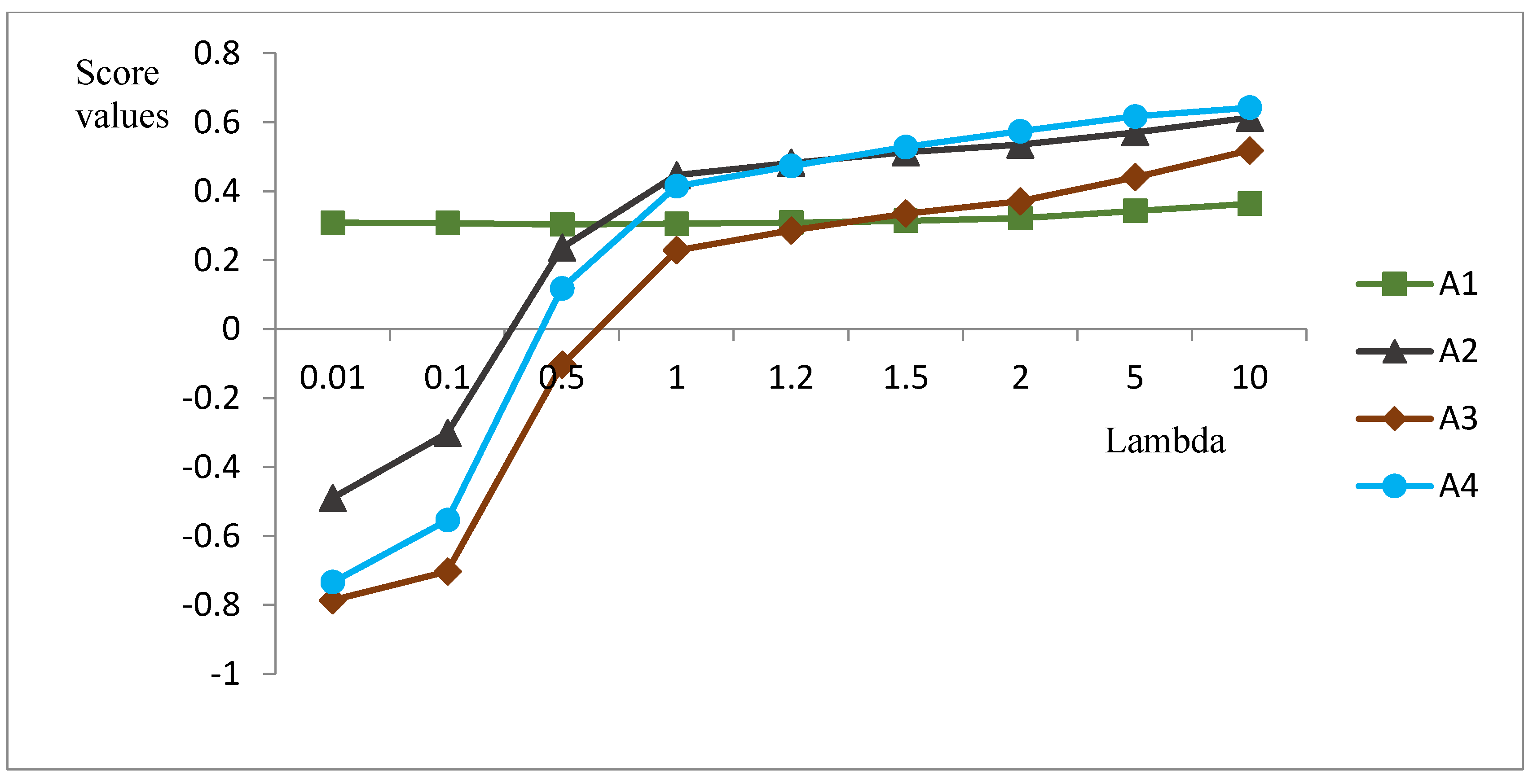
To observe the influence of the parameter value $\lambda$ for this example, we can adopt the different value $\lambda$ in Step (5) to obtain the rankings of the alternatives, which are shown in

Table 3. Ranking sensitivity analysis based on different parameter $\lambda$ in NIFGWPIA operator.

$\mathit{\lambda }$	Comprehensive Evaluation Value ${\stackrel{⌢}{\mathit{z}}}_{\mathit{i}}$	Score Functions ${\mathit{s}}_1({\stackrel{⌢}{\mathit{z}}}_{\mathit{i}})$	Ranking
$\lambda =0.01$	$\begin{array}{l}{\stackrel{⌢}{z}}_1=\langle (0.8470,0.0777),0.6195,0.2552\rangle \\ {\stackrel{⌢}{z}}_2=\langle 0.8801,0.0541),0.2221,0.7779\rangle \\ {\stackrel{⌢}{z}}_3=\langle 0.8210,0.0512),0.0212,0.9788\rangle \\ {\stackrel{⌢}{z}}_4=\langle 0.8822,0.0604),0.0843,0.9157\rangle \end{array}$	$\begin{array}{l}{s}_1\left({\stackrel{⌢}{z}}_1\right)=0.3086\\ s_1\left({\stackrel{⌢}{z}}_2\right)=-0.4892\\ s_1\left({\stackrel{⌢}{z}}_3\right)=-0.7861\\ s_1\left({\stackrel{⌢}{z}}_4\right)=-0.7334\end{array}$	$e_1\succ e_2\succ e_4\succ e_3$
$\lambda =0.1$	$\begin{array}{l}{\stackrel{⌢}{z}}_1=\langle (0.8475,0.0776),0.6190,0.2556\rangle \\ {\stackrel{⌢}{z}}_2=\langle (0.8806,0.0543),0.3288,0.6712\rangle \\ {\stackrel{⌢}{z}}_3=\langle (0.8212,0.0513),0.0719,0.9281\rangle \\ {\stackrel{⌢}{z}}_4=\langle (0.8825,0.0602),0.1862,0.8138\rangle \end{array}$	$\begin{array}{l}{s}_1\left({\stackrel{⌢}{z}}_1\right)=0.3080\\ s_1\left({\stackrel{⌢}{z}}_2\right)=-0.3015\\ s_1\left({\stackrel{⌢}{z}}_3\right)=-0.7031\\ s_1\left({\stackrel{⌢}{z}}_4\right)=-0.5539\end{array}$	$e_1\succ e_2\succ e_4\succ e_3$
$\lambda =0.5$	$\begin{array}{l}{\stackrel{⌢}{z}}_1=\langle (0.8516,0.0767),0.6158,0.2588\rangle \\ {\stackrel{⌢}{z}}_2=\langle (0.8845,0.0556),0.6338,0.3662\rangle \\ {\stackrel{⌢}{z}}_3=\langle (0.8229,0.0521),0.4371,0.5629\rangle \\ {\stackrel{⌢}{z}}_4=\langle (0.8852,0.0592),0.5672,0.4328\rangle \end{array}$	$\begin{array}{l}{s}_1\left({\stackrel{⌢}{z}}_1\right)=0.3040\\ s_1\left({\stackrel{⌢}{z}}_2\right)=0.2366\\ s_1\left({\stackrel{⌢}{z}}_3\right)=-0.1035\\ s_1\left({\stackrel{⌢}{z}}_4\right)=0.1190\end{array}$	$e_1\succ e_2\succ e_4\succ e_3$
$\lambda =1.0$	$\begin{array}{l}{\stackrel{⌢}{z}}_1=\langle (0.8565,0.0757),0.6162,0.2585\rangle \\ {\stackrel{⌢}{z}}_2=\langle (0.8894,0.0572),0.7510,0.2490\rangle \\ {\stackrel{⌢}{z}}_3=\langle (0.8250,0.0532),0.6387,0.3613\rangle \\ {\stackrel{⌢}{z}}_4=\langle (0.8885,0.0580),0.7334,0.2666\rangle \end{array}$	$\begin{array}{l}{s}_1\left({\stackrel{⌢}{z}}_1\right)=0.3063\\ s_1\left({\stackrel{⌢}{z}}_2\right)=0.4465\\ s_1\left({\stackrel{⌢}{z}}_3\right)=0.2288\\ s_1\left({\stackrel{⌢}{z}}_4\right)=0.4147\end{array}$	$e_2\succ e_4\succ e_1\succ e_3$
$\lambda =1.2$	$\begin{array}{l}{\stackrel{⌢}{z}}_1=\langle (0.8583,0.0754),0.6176,0.2571\rangle \\ {\stackrel{⌢}{z}}_2=\langle (0.8913,0.0579),0.7708,0.2292\rangle \\ {\stackrel{⌢}{z}}_3=\langle (0.8259,0.0536),0.6734,0.3266\rangle \\ {\stackrel{⌢}{z}}_4=\langle (0.8898,0.0575),0.7659,0.2341\rangle \end{array}$	$\begin{array}{l}{s}_1\left({\stackrel{⌢}{z}}_1\right)=0.3094\\ s_1\left({\stackrel{⌢}{z}}_2\right)=0.4828\\ s_1\left({\stackrel{⌢}{z}}_3\right)=0.2864\\ s_1\left({\stackrel{⌢}{z}}_4\right)=0.4733\end{array}$	$e_2\succ e_4\succ e_1\succ e_3$
$\lambda =1.5$	$\begin{array}{l}{\stackrel{⌢}{z}}_1=\langle (0.8611,0.0749),0.6201,0.2546\rangle \\ {\stackrel{⌢}{z}}_2=\langle (0.8942,0.0588),0.7871,0.2129\rangle \\ {\stackrel{⌢}{z}}_3=\langle (0.8271,0.0543),0.7027,0.2973\rangle \\ {\stackrel{⌢}{z}}_4=\langle (0.8917,0.0568),0.7965,0.2035\rangle \end{array}$	$\begin{array}{l}{s}_1\left({\stackrel{⌢}{z}}_1\right)=0.3147\\ s_1\left({\stackrel{⌢}{z}}_2\right)=0.5135\\ s_1\left({\stackrel{⌢}{z}}_3\right)=0.3353\\ s_1\left({\stackrel{⌢}{z}}_4\right)=0.5288\end{array}$	$e_4\succ e_2\succ e_3\succ e_1$
$\lambda =2.0$	$\begin{array}{l}{\stackrel{⌢}{z}}_1=\langle (0.8654,0.0744),0.6237,0.2510\rangle \\ {\stackrel{⌢}{z}}_2=\langle (0.8988,0.0603),0.7978,0.2022\rangle \\ {\stackrel{⌢}{z}}_3=\langle (0.8292,0.0553),0.7240,0.2760\rangle \\ {\stackrel{⌢}{z}}_4=\langle (0.8949,0.0556),0.8208,0.1792\rangle \end{array}$	$\begin{array}{l}{s}_1\left({\stackrel{⌢}{z}}_1\right)=0.3226\\ s_1\left({\stackrel{⌢}{z}}_2\right)=0.5354\\ s_1\left({\stackrel{⌢}{z}}_3\right)=0.3715\\ s_1\left({\stackrel{⌢}{z}}_4\right)=0.5742\end{array}$	$e_4\succ e_2\succ e_3\succ e_1$
$\lambda =5.0$	$\begin{array}{l}{\stackrel{⌢}{z}}_1=\langle (0.8869,0.0737),0.6308,0.2439\rangle \\ {\stackrel{⌢}{z}}_2=\langle (0.9228,0.0678),0.8093,0.1907\rangle \\ {\stackrel{⌢}{z}}_3=\langle (0.8409,0.0618),0.7622,0.2378\rangle \\ {\stackrel{⌢}{z}}_4=\langle (0.9126,0.0496),0.8384,0.1616\rangle \end{array}$	$\begin{array}{l}{s}_1\left({\stackrel{⌢}{z}}_1\right)=0.3431\\ s_1\left({\stackrel{⌢}{z}}_2\right)=0.5708\\ s_1\left({\stackrel{⌢}{z}}_3\right)=0.4410\\ s_1\left({\stackrel{⌢}{z}}_4\right)=0.6176\end{array}$	$e_4\succ e_2\succ e_3\succ e_1$
$\lambda =10.0$	$\begin{array}{l}{\stackrel{⌢}{z}}_1=\langle (0.9116,0.0765),0.6369,0.2378\rangle \\ {\stackrel{⌢}{z}}_2=\langle (0.9491,0.0745),0.8231,0.1769\rangle \\ {\stackrel{⌢}{z}}_3=\langle (0.8566,0.0708),0.8026,0.1974\rangle \\ {\stackrel{⌢}{z}}_4=\langle (0.9353,0.0438),0.8435,0.1565\rangle \end{array}$	$\begin{array}{l}{s}_1\left({\stackrel{⌢}{z}}_1\right)=0.3639\\ s_1\left({\stackrel{⌢}{z}}_2\right)=0.6134\\ s_1\left({\stackrel{⌢}{z}}_3\right)=0.5184\\ s_1\left({\stackrel{⌢}{z}}_4\right)=0.6426\end{array}$	$e_4\succ e_2\succ e_3\succ e_1$

and Figure 1.

In Table 3, we can see the best alternative is different for the different value $\lambda$ in NIFGWPIA operator. Further, we can give the following analysis.

When parameter $\lambda$ increases ($\lambda \ge 0.5$), the MD in comprehensive value ${\stackrel{⌢}{z}}_i$ will increase, and the NMD will decrease. Thus, we can regard parameter $\lambda$ as a risk attitude value. When decision maker is the type of risk aversion (or called the conservative type), a little value of $\lambda$ can be adopted; when decision maker is the type of risk seeking (or called the aggressive type), a big value of $\lambda$ can be used. In general, when $\lambda =1$, we can think it is neutral. Thus, in this example, we can select the best is $e_4$ when $\lambda \ge 1.5$; or best is $e_2$ when $\lambda$ is approximately one; or the best is $e_1$ when $\lambda \le 0.5$.

Comparing with the method proposed by Wang et al. [23], there are the same ranking results $e_4$ and $e_2$. However, we also give another ranking result, i.e., the best may be $e_1$ when $\lambda \le 0.5$. The advantages of the developed method in this paper are that it considers the relationships of different attribute values by PA operator and the interaction between the MD and NMD, and the advantages of the developed method by Wang et al. [23] are that it considers the OWA and the induced variables.

Comparing with the method proposed by Wang and Li [15], the advantages of the developed method in this paper are that it can give the comprehensive value of each alternative based on the power interaction averaging operators of NIFNs by considering the relationships of different attributes and the interaction between the MD and NMD, and the advantages of the method proposed by Wang and Li [15] are that it can solve the MADM problems with incomplete weight information, however, it can only give the ranking result by TOPSIS, and not comprehensive value.

Comparing with the method proposed by Wang and Li [14], Wang and Li [14] also proposed some aggregation operators, especially some intuitionistic normal fuzzy related weighted averaging operators. However, we think that, if there exists relationships between attributes, the operational laws in NFNs may be incorrect because these operational laws need the condition that the attributes are independent. The aggregation operators and method propose in this paper can only consider the relations of attribute values by PA operator, and still keep the condition that the attributes are independent.

7. Conclusions

In this paper, we firstly defined some basic operational rules of NIFNs by the interaction operations of IFNs, and then we proposed some new aggregation operators for NIFNs. Further, we studied their properties and some special cases, and proposed a MADM approach for the decision information in NIFNs based on the NIFGWPIA operator. The significant characteristics of the proposed method are that: (1) it is easier to describe the uncertain information than the existing fuzzy sets and stochastic variables; (2) it used the interaction operations in part of IFSs which could overcome the existing weaknesses in operational rules of NIFNs; (3) it adopted PA operator which could relieve the influence of unreasonable data given by biased decision makers; and (4) it made the decision-making results more flexible and reliable because it was with generalized parameter that could be regarded as the risk attitude value of decision makers. In the future, we will study the applications of the proposed operators and method for the MADM problems with normal distribution stochastic information [37,38], especially for supply chain managements [39] and inventory models [40,41], or study the fuzzy graphs or trees based on NIFNs [42,43,44,45].

References

1. Zadeh, L.A. Fuzzy sets. Inf. Control 1965, 8, 338–356. [Google Scholar] [CrossRef]
2. Atanassov, K.T. Intuitionistic fuzzy sets. Fuzzy Sets Syst. 1986, 20, 87–96. [Google Scholar] [CrossRef]
3. Biswas, A.; De Kumar, A. An efficient ranking technique for intuitionistic fuzzy numbers with its application in chance constrained bilevel programming. Adv. Fuzzy Syst. 2016, 2016, 6475403. [Google Scholar] [CrossRef]
4. Atanassov, K.T.; Gargov, G. Interval-valued intuitionistic fuzzy sets. Fuzzy Sets Syst. 1989, 3, 343–349. [Google Scholar] [CrossRef]
5. Zhang, X.; Liu, P.D. Method for aggregating triangular intuitionistic fuzzy information and its application to decision making. Technol. Econ. Dev. Econ. 2010, 16, 280–290. [Google Scholar] [CrossRef]
6. Shu, M.H.; Cheng, C.H.; Chang, J.R. Using intuitionistic fuzzy sets for fault-tree analysis on printed circuit board assembly. Microelectron. Reliab. 2006, 46, 2139–2148. [Google Scholar] [CrossRef]
7. Wang, J.Q. Overview on fuzzy multi-criteria decision-making approach. Control Decis. 2008, 23, 601–606. [Google Scholar]
8. Wang, J.Q.; Li, J.J. The multi-criteria group decision making method based on multi-granularity intuitionistic two semantics. Sci. Technol. Inf. 2009, 33, 8–9. [Google Scholar]
9. Liu, P.D.; Jin, F. Methods for aggregating intuitionistic uncertain linguistic variables and their application to group decision making. Inf. Sci. 2012, 205, 58–71. [Google Scholar] [CrossRef]
10. Liu, P.D.; Liu, Z.M.; Zhang, X. Some intuitionistic uncertain linguistic heronian mean operators and their application to group decision making. Appl. Math. Comput. 2014, 230, 570–586. [Google Scholar] [CrossRef]
11. Liu, P.D. Some geometric aggregation operators based on interval intuitionistic uncertain linguistic variables and their application to group decision making. Appl. Math. Model. 2013, 37, 2430–2444. [Google Scholar] [CrossRef]
12. Atanassov, K. New operations defined over the intuitionistic fuzzy sets. Fuzzy Sets Syst. 1994, 61, 137–142. [Google Scholar] [CrossRef]
13. He, Y.D.; Chen, H.Y.; Zhou, L.G.; Han, B.; Zhao, Q.Y.; Liu, J.P. Generalized intuitionistic fuzzy geometric interaction operators and their application to decision making. Expert Syst. Appl. 2014, 41, 2484–2495. [Google Scholar] [CrossRef]
14. Wang, J.Q.; Li, K.J. Multi-criteria decision-making method based on induced intuitionistic normal fuzzy related aggregation operators. Int. J. Uncertain. Fuzziness Knowl. Based Syst. 2012, 20, 559–578. [Google Scholar] [CrossRef]
15. Wang, J.Q.; Li, K.J. Multi-criteria decision-making method based on intuitionistic normal fuzzy aggregation operators. Syst. Eng. Theory Pract. 2013, 33, 1501–1508. [Google Scholar]
16. Yang, M.S.; Ko, C.H. On a class of fuzzy c-numbers clustering procedures for fuzzy data. Fuzzy Sets Syst. 1996, 84, 49–60. [Google Scholar] [CrossRef]
17. Xie, N.; Li, Z.; Zhang, G. An intuitionistic fuzzy soft set method for stochastic decision-making applying prospect theory and grey relational analysis. J. Intell. Fuzzy Syst. 2017, 33, 15–25. [Google Scholar] [CrossRef]
18. Li, P.; Yang, Y.; Wei, C. An intuitionistic fuzzy stochastic decision-making method based on case-based reasoning and prospect theory. Math. Probl. Eng. 2017, 2017, 2874954. [Google Scholar] [CrossRef]
19. Gao, J.; Liu, H. Interval-valued intuitionistic fuzzy stochastic multi-criteria decision-making method based on Prospect theory. Kybernetes 2015, 44, 25–42. [Google Scholar] [CrossRef]
20. Keshavarz Ghorabaee, M.; Amiri, M.; Zavadskas, E.K.; Turskis, Z.; Antucheviciene, J. Stochastic EDAS method for multi-criteria decision-making with normally distributed data. J. Intell. Fuzzy Syst. 2017, 33, 1627–1638. [Google Scholar] [CrossRef]
21. Zhou, H.; Wang, J.Q.; Zhang, H.Y. Grey stochastic multi-criteria decision-making based on regret theory and TOPSIS. Int. J. Mach. Learn. Cybern. 2017, 8, 651–664. [Google Scholar] [CrossRef]
22. Li, D.Y.; Liu, C.Y. Study on the universality of the normal cloud model. Eng. Sci. 2004, 6, 28–34. [Google Scholar]
23. Wang, J.Q.; Zhou, P.; Li, K.J.; Zhang, H.Y.; Chen, X.H. Multi-criteria decision-making method based on normal intuitionistic fuzzy-induced generalized aggregation operator. TOP 2014, 22, 1103–1122. [Google Scholar] [CrossRef]
24. Yager, R.R. The power average operator. IEEE Trans. Syst. Man Cybern. Part A Syst. Hum. 2001, 31, 724–731. [Google Scholar] [CrossRef]
25. Xu, Z.S.; Yager, R.R. Power-Geometric operators and their use in group decision making. IEEE Trans. Fuzzy Syst. 2010, 18, 94–105. [Google Scholar]
26. Xu, Z.S. Approaches to multiple attribute group decision making based on intuitionistic fuzzy power aggregation operators. Knowl. Based Syst. 2011, 24, 749–760. [Google Scholar] [CrossRef]
27. Zhou, L.G.; Chen, H.Y. A generalization of the power aggregation operators for linguistic environment and its application in group decision making. Knowl. Based Syst. 2012, 26, 216–224. [Google Scholar] [CrossRef]
28. Zhang, Z.M. Hesitant fuzzy power aggregation operators and their application to multiple attribute group decision making. Inf. Sci. 2013, 234, 150–181. [Google Scholar] [CrossRef]
29. Liu, P.D.; Yu, X.C. 2-dimension uncertain linguistic power generalized weighted aggregation operator and its application for multiple attribute group decision making. Knowl. Based Syst. 2014, 57, 69–80. [Google Scholar] [CrossRef]
30. Liu, P.D.; Wang, Y.M. Multiple attribute group decision making methods based on intuitionistic linguistic power generalized aggregation operators. Appl. Soft Comput. 2014, 17, 90–104. [Google Scholar] [CrossRef]
31. Liu, P.D.; Liu, Y. An approach to multiple attribute group decision making based on intuitionistic trapezoidal fuzzy power generalized aggregation operator. Int. J. Comput. Intell. Syst. 2014, 7, 291–304. [Google Scholar] [CrossRef]
32. Keshavarz Ghorabaee, M.; Amiri, M.; Zavadskas, E.K.; Turskis, Z. A new hybrid simulation-based assignment approach for evaluating airlines with multiple service quality criteria. J. Air Transp. Manag. 2017, 63, 45–60. [Google Scholar] [CrossRef]
33. Aydogan, E.K.; Ozmen, M. The stochastıc vikor method and its use in reverse logistic option selection problem. RAIRO Oper. Res. 2017, 51, 375–389. [Google Scholar] [CrossRef]
34. Zhao, H.; Li, N. Performance evaluation for sustainability of strong smart grid by using stochastic AHP and fuzzy TOPSIS methods. Sustainability 2016, 8, 129. [Google Scholar] [CrossRef]
35. Sarkar, B. A production-inventory model with probabilistic deterioration in two-echelon supply chain management. Appl. Math. Model. 2013, 37, 3138–3151. [Google Scholar] [CrossRef]
36. Xu, R.N.; Li, C.L. Regression prediction for fuzzy time series. Appl. Math. A J. Chin. Univ. Ser. A 2001, 16, 451–461. (In Chinese) [Google Scholar]
37. Habib, M.S.; Sarkar, B. An integrated location-allocation model for temporary disaster debris management under an uncertain environment. Sustainability 2017, 9, 716. [Google Scholar] [CrossRef]
38. Soni, H.N.; Sarkar, B.; Mahapatra, A.; Majumder, S. Lost sales reduction and quality improvement with variable lead time and fuzzy costs in an imperfect production system. RAIRO Oper. Res. 2017, in press. [Google Scholar] [CrossRef]
39. Sarkar, B. Supply chain coordination with variable backorder, inspections, and discount policy for fixed lifetime products. Math. Probl. Eng. 2016, 2016, 6318737. [Google Scholar] [CrossRef]
40. Sarkar, B.; Mahapatra, A.S. Periodic review fuzzy inventory models with variable lead time and fuzzy demand. Int. Trans. Oper. Res. 2017, 24, 1197–1227. [Google Scholar] [CrossRef]
41. Soni, H.N.; Sarkar, B.; Joshi, M. Demand uncertainty and learning in fuzziness in a continuous review inventory model. J. Intell. Fuzzy Syst. 2017, 33, 2595–2608. [Google Scholar] [CrossRef]
42. Pramanik, T.; Samanta, S.; Sarkar, M. Pal, Fuzzy φ-tolerance competition Graphs. Soft Comput. 2017, 21, 3723–3734. [Google Scholar]
43. Pramanik, T.; Samanta, S.; Pal, M.; Mondal, S.; Sarkar, B. Interval-valued fuzzy ϕ-tolerance competition graphs. Springer Plus 2016, 5, 1981. [Google Scholar] [CrossRef] [PubMed]
44. Samanta, S.; Sarkar, B.; Shin, D.; Pal, M. Completeness and regularity of generalized fuzzy graphs. Springer Plus 2016, 5, 1979. [Google Scholar] [CrossRef] [PubMed]
45. Sarkar, B.; Samanta, S. Generalized Fuzzy Trees. J. Comput. Intell. Syst. 2017, 10, 711–720. [Google Scholar] [CrossRef]
Figure 1. Ranking sensitivity analysis based on different parameter λ in NIFGWPIA operator.
Symmetry 09 00261 g001