The Development of Improved Incremental Models Using Local Granular Networks with Error Compensation


1
Department of Control and Instrumentation Engineering, Chosun University, Gwangju 61452, Korea
2
Department of Electronics Engineering, Chosun University, Gwangju 61452, Korea
*
Author to whom correspondence should be addressed.
Symmetry 2017, 9(11), 266; https://doi.org/10.3390/sym9110266
Submission received: 1 October 2017
/
Revised: 25 October 2017
/
Accepted: 1 November 2017
/
Published: 5 November 2017
(This article belongs to the Special Issue Symmetry in Fuzzy Sets and Systems)
Abstract
:In this paper, we use the fundamental idea of the incremental model (IM) and develop the design framework. The design method of IM is composed of two steps. In the first step, we perform a linear regression (LR) as the global model. In the second step, the errors obtained by the global model are predicted by fuzzy if-then rules generated through a local linguistic model. Although the effectiveness of IM has been demonstrated in various prediction examples, we propose an improved incremental model (IIM) to deal with complex nonlinear characteristics. For this purpose, we employ adaptive neuro-fuzzy networks (ANFN) or radial basis function networks (RBFN) to create local granular networks in the design of IIM. Furthermore, we use quadratic regression (QR) as a global model, because linear relationship of LR may not hold in many settings. Numerical studies concern four datasets (automobile data, energy efficiency data, Boston housing data and computer hardware data). The experimental results demonstrate that IIM outperformed the previous models.
1. Introduction
The past few decades have witnessed several studies in various real-world problems of fuzzy logic [1]. The issues of interpretability and transparency are still open, while the accuracy of fuzzy models has been treated in several studies [2]. For this purpose, various clustering algorithms have been employed in fuzzy modeling. However, these techniques are used to generate knowledge information from numerical data. The well-known clustering-based techniques in the design of the fuzzy inference system are hard c-means clustering, clustering introduced by Bezdek [3], clustering introduced by Chiu [4], Gustafson–Kessel fuzzy clustering [5] and Gath–Geva clustering [6]. Recently, several studies using clustering methods have been done on system modeling [7,8,9]. These context-free clustering algorithms estimate the cluster centers without considering the characteristics between the input and output.
Meanwhile, context-based clustering estimates cluster centers, preserving homogeneity in the input attributes and the output [10]. The validity of these clustering methods has been presented in the previous literature [11,12,13,14,15]. Among these models, the incremental model (IM) represented the unique properties in contrast to the conventional methods. The IM is designed by the combination of the linear part as the global scheme and knowledge representation as the local scheme [14]. Recently, an expansion of IM was presented [16].
However, the problem of performance degradation may be encountered when a system to be modeled has complex nonlinear characteristics, although the effectiveness of the IM has been demonstrated in various prediction examples. In the design of IM, the Linguistic Model (LM) is similar to the fuzzy models of Mamdani [17] in that the premise and consequent membership functions are all fuzzy. For that reason, we need more advanced local granular networks with the aid of information granulation. Furthermore, the linear relationship of LR may not hold in many settings. To deal with the nonlinear relationship in the design of the global model, we employ quadratic regression (QR) instead of LR. Therefore, we use two networks to design local networks in the construction of IM. Here, these networks are constructed by Context-based Fuzzy C-Means (CFCM) clustering with the aid of information granulation. Consequently, two different networks based on fuzzy granulation are developed. Thus, the errors obtained by QR are predicted by radial basis functions or Takagi–Sugeno–Kang (TSK)-type fuzzy rules. The remarkable generalization capability of the improved incremental model (IIM) is derived from the following facts: The IIM can achieve a highly nonlinear mapping by using the combination of QR and local granular networks. The IIM also has fuzzy if-then rules and adjustable parameters, far fewer than those used in the design of LM. We shall use automobile fuel consumption, an energy example, Boston housing data and computer hardware available from machine learning examples.
In Section 2, the concept and design procedure of IM are presented. The IM consists of several computing paradigms, including LR as a global model and local LM realized by specialized CFCM clustering. In Section 3, the two types, incremental radial basis function networks (IRBFN) and Incremental adaptive neuro-fuzzy networks (IANFN), are described. Here, we explain QR as a global model and the design procedure of the proposed methods. In Section 4, the experiments are performed on four datasets. The conclusion and comments are described in Section 5.
2. Incremental Model Based on LR and Local LM
The IM constituents are composed of CFCM clustering, LR as a global model and LM as a local model. Each of these constituent methodologies has its own strength. The seamless integration of these methodologies forms the core of IM design.
2.1. The Description of IM
Figure 1 visualizes the underlying concept of IM. Here, the dataset is approximated by the LR in the linear part. However, LR is not suitable for predicting in this example. These elliptical parts are performed through the local model based on CFCM clustering.
2.2. CFCM Clustering
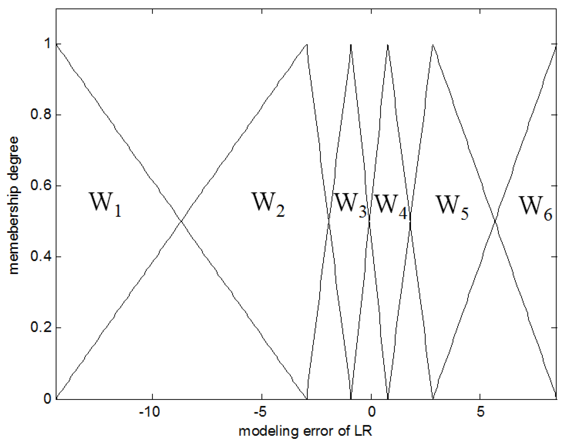
The CFCM clustering is performed between the input attributes and the error obtained from the LR. These errors are used as output in the design of local LM. Figure 2 shows the contexts generated in the error space. As shown in Figure 2, the number of contexts is six. These contexts are characterized by linguistic labels such as negative small error, positive small error, and so on. These contexts are characterized by triangular membership functions. These are produced by the context generation method [18].
In what follows, the estimation method of clusters based on CFCM clustering is presented. The CFCM clustering estimates the cluster centers representing characteristics between input attributes and errors. The membership matrix is composed of degrees with a value between zero and one as the following equation.
The cost function for CFCM clustering is computed as follows:
The membership matrix is defined as follows:
The cluster centers are calculated as follows:
2.3. The Design Procedure of IM
The design procedure of IM can be performed via five steps.
- Step 1: Construct LR from input-output data pairs. LR performs the task of fitting data using a linear model. After performing the regression, we obtain the input and error pairs, ().
- Step 2: Generate the contexts in the error space.
- Step 3: Estimate cluster centers by CFCM clustering.
- Step 4: The final output of LM is expressed as:
- Step 5: Obtain the model output by combining the outputs of LR and LM.
The fuzzy rules are given in the if-then form as follows:
3. Improved Incremental Models Using Local Granular Networks
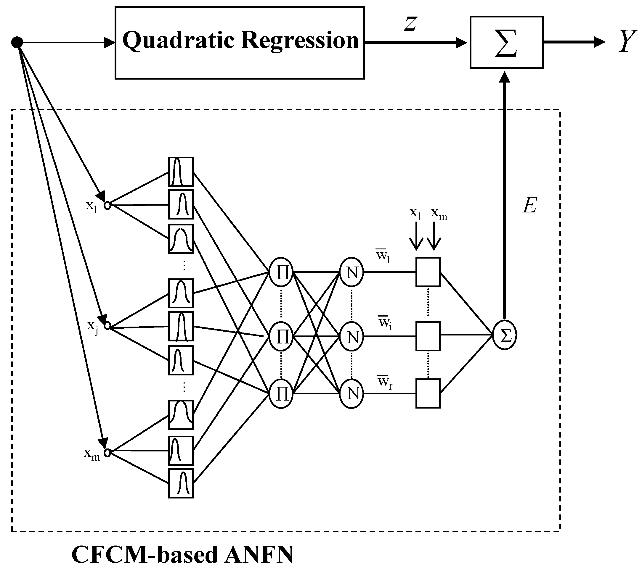
In this section, we design local granular networks based on ANFN and RBFN for the construction of IIM. In the design of LR, a linear relationship may not hold in various applications where the system has complex nonlinear characteristics. To deal with the nonlinear relationship in the design of the global model, we employ QR instead of LR. Thus, we use a QR in the following form:
Figure 4 visualizes the concept of IIM-based QR and local granular networks. We firstly use the QR model. Then, the remaining nonlinear areas are predicted by radial basis functions or TSK-type fuzzy rules represented by RBFN or ANFN. Figure 4 visualizes the concept of IIM using QR and local granular networks.
3.1. Incremental RBFN
The proposed IRBFN is presented in Figure 5. The IRBFN is constructed via a similar procedure as that of IM. Here, the clusters estimated by CFCM clustering are used as the radial basis functions in the hidden layer of the local RBFN. The local granular network is represented by the linear relation between the receptive fields and the weights as follows:
The learning methods are implemented in two ways. In the first scheme, the parameters between the hidden and the output layer are obtained by the least-square estimator, when the parameters in the hidden layer are fixed. Next, the parameters such as the weights and cluster centers are adjusted by the BP (Back-Propagation) algorithm. The output of the IRBFN is obtained by the combination of QR and local RBFN as follows:
The pseudocode in the design of the proposed IRBFN is shown below.
Initial setting:
- Divide randomly for the training and testing data.
- Normalize the input data between zero and one.
- Design QR as the global model and obtain the modeling error.
Processing: iterate .
- Set the number of contexts and clusters.
- Generate the contexts in the error space.
- Design local RBFN using CFCM clustering to compensate the error.
- Estimate the weights of the output layer based on the LSE method as one-pass; or adjust the centers estimated by CFCM and initial weights using the BP algorithm.
- Obtain the output of the local RBFN.
Final output: Combine the output of local RBFN with QR.
3.2. Incremental ANFN
Figure 6 shows the architecture of the proposed IANFN. The IANFN is designed by QR and local TSK-type ANFN. The first layer of ANFN is constructed by the CFCM clustering as the scatter partitioning.
For simplicity, we consider the TSK-type fuzzy model. The network output is computed as follows:
Figure 7 visualizes the schema of the proposed IANFN.
4. Experimental Results
In this section, we use four different datasets. These data pairs are randomly divided into the training (60%) and testing (40%) dataset, respectively. The experiment is also repeated 10 times [19]. The prediction performances are measured by the conventional RMSE (Root Mean Squared Error) as follows:
where and are the model output and actual target output, respectively.
4.1. Automobile MPG Dataset
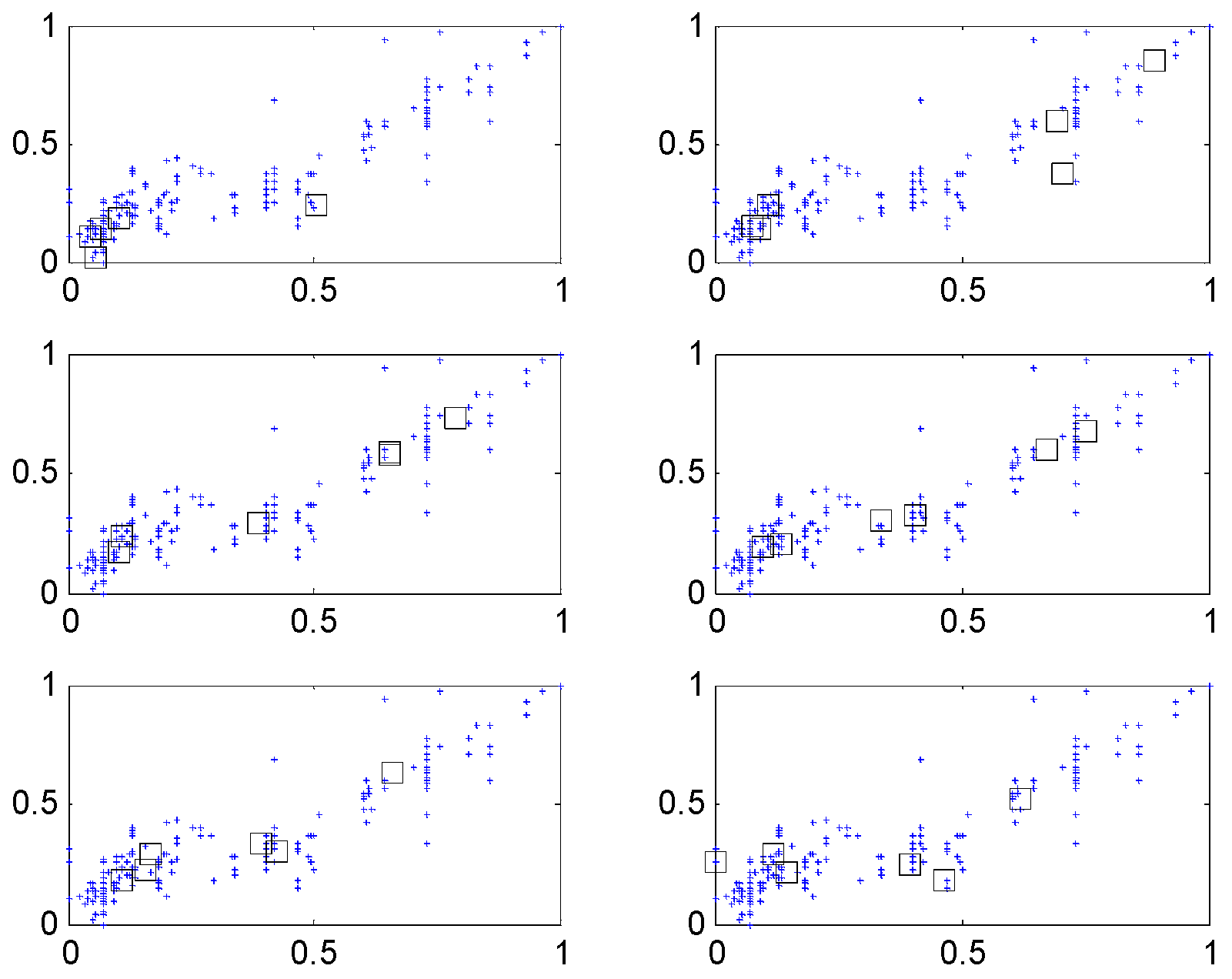
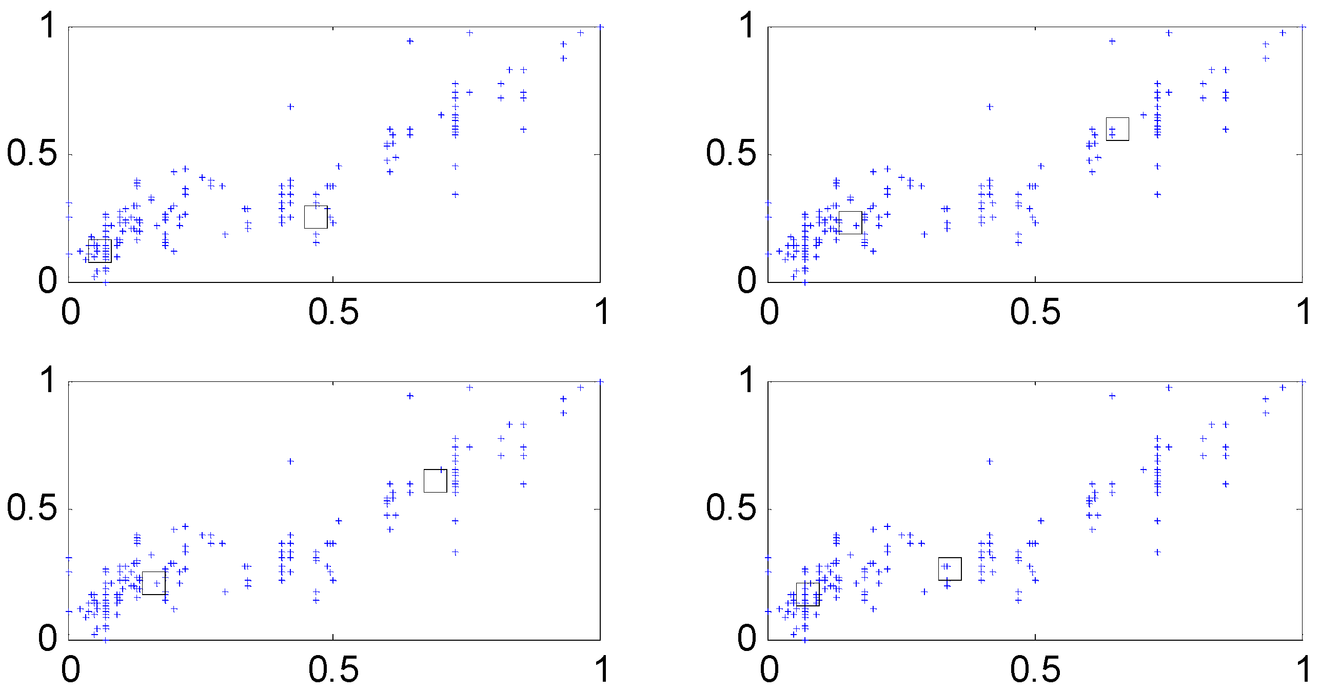
The input attributes consist of weight, acceleration, model year, cylinder number, displacement and horsepower [20,21]. We randomly divided the dataset into training and testing datasets. For simplicity, the IM is constructed by p = c = 6, when LR is used as the global model. Figure 8 shows the contexts generated by the error. Each context is expressed by a triangular fuzzy set representing linguistic labels. Figure 9 visualizes the cluster centers corresponding to each context shown in Figure 8. In Figure 8, the circles and squares denote the data and centers, respectively. Furthermore, each axis denotes the displacement and horsepower, respectively.
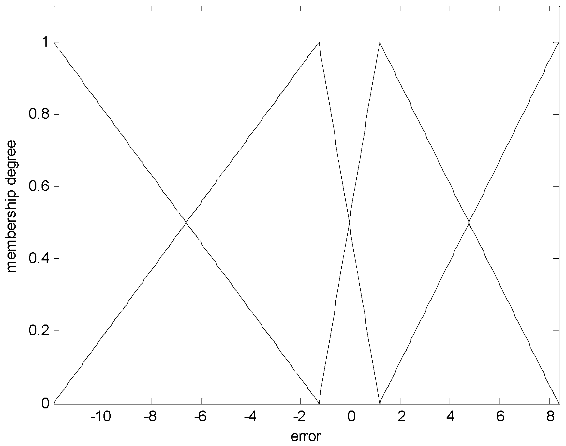
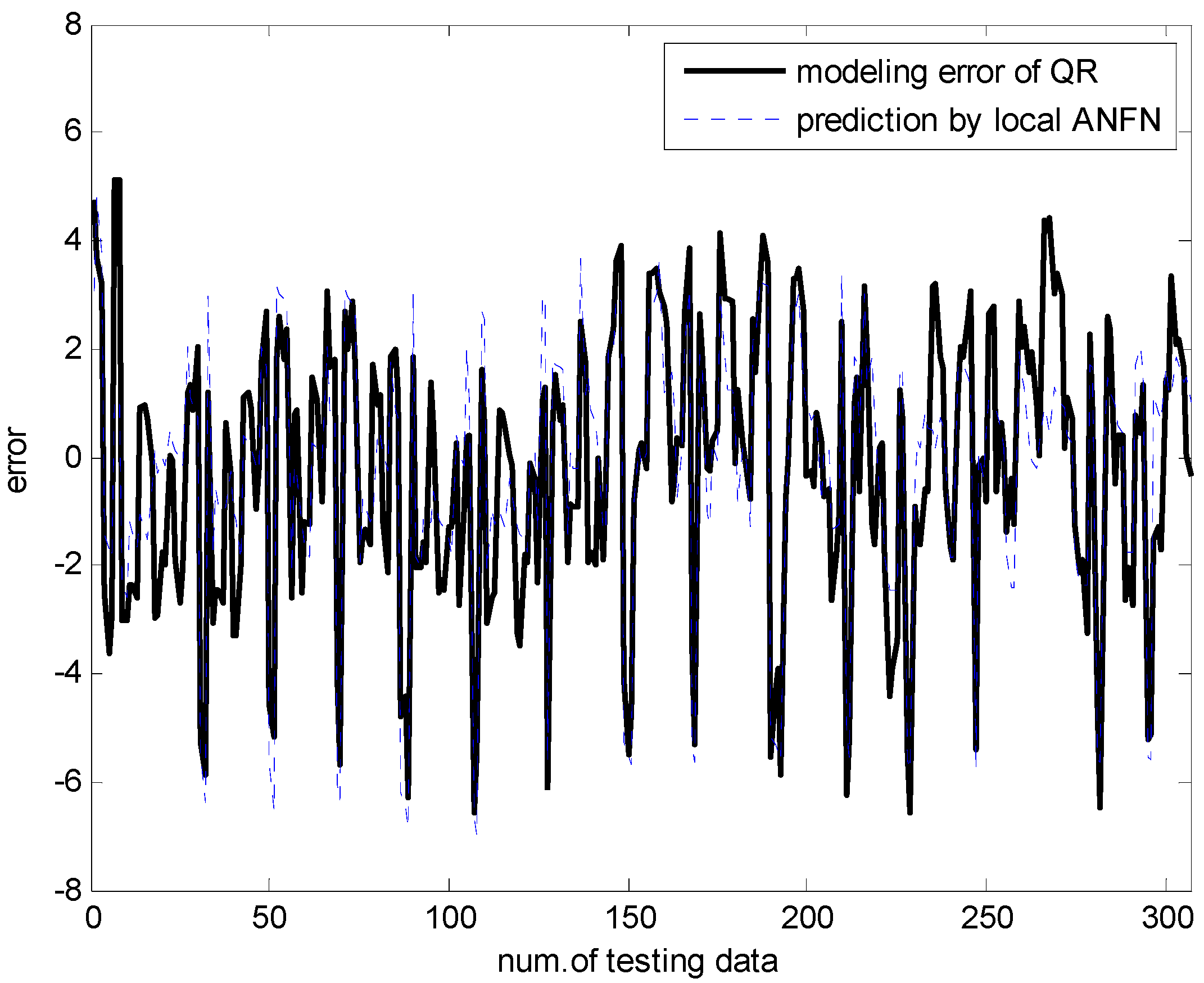
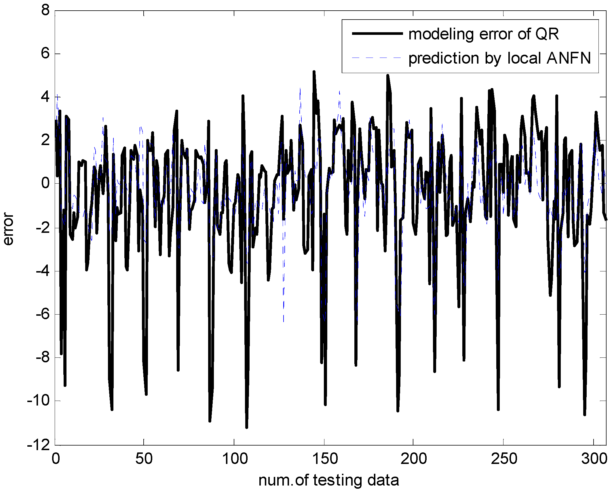
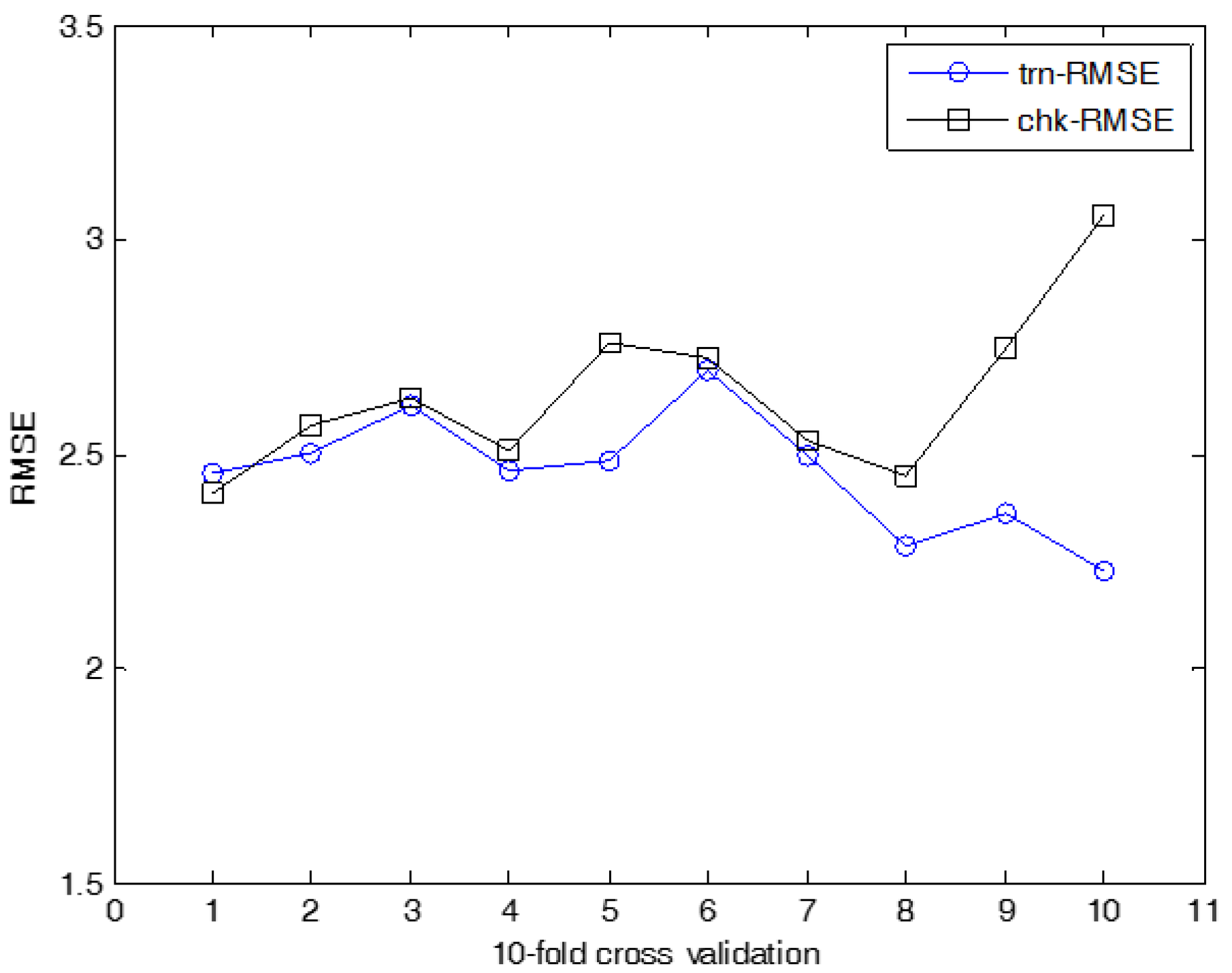
In what follows, we performed the experiments on an IRBFN with two types (LSE, BP) and an IANFN, when the global model is QR. In the design of the IRBFN and IANFN, we selected p = c = 3 and p = 4, c = 2, showing a good generalization performance, respectively. Figure 10 shows four contexts generated from the error space in the case of the IANFN. Figure 11 shows the cluster centers corresponding to each context shown in Figure 10. Figure 12 shows the simulation result of the proposed IANFN. Table 1 lists the RMSE values of the proposed approach and the previous methods. Here the trn-RMSE and chk-RMSE denote the RMSE for training and testing data set, respectively. The average values of RMSE were calculated by 10-fold cross validation [22]. The IIM performed well in comparison to the previous methods. Here, the proposed IANFN achieved the best performance in the generalization capability. The IIM obviously outperformed the IRBFN and IANFN based on LR, as well as the previous methods. Moreover, it was found from the results that the IIM had fuzzy if-then rules and adjustable parameters, far fewer than those used in the design of LM itself without using LR. The result clearly showed that the fundamental IM was improved by IRBFN and IANFN with LR or QR as the global model.
4.2. Energy Efficiency Data
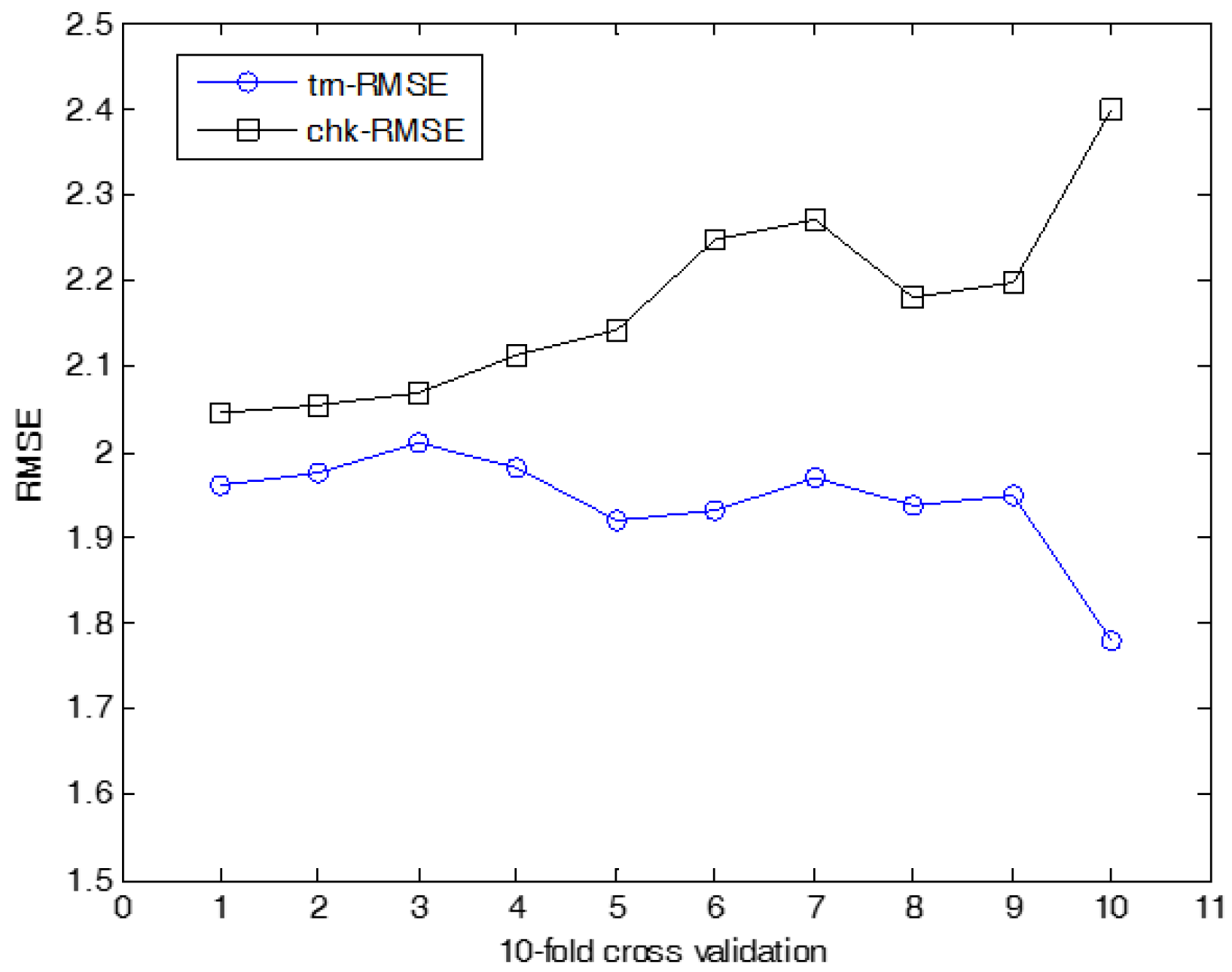
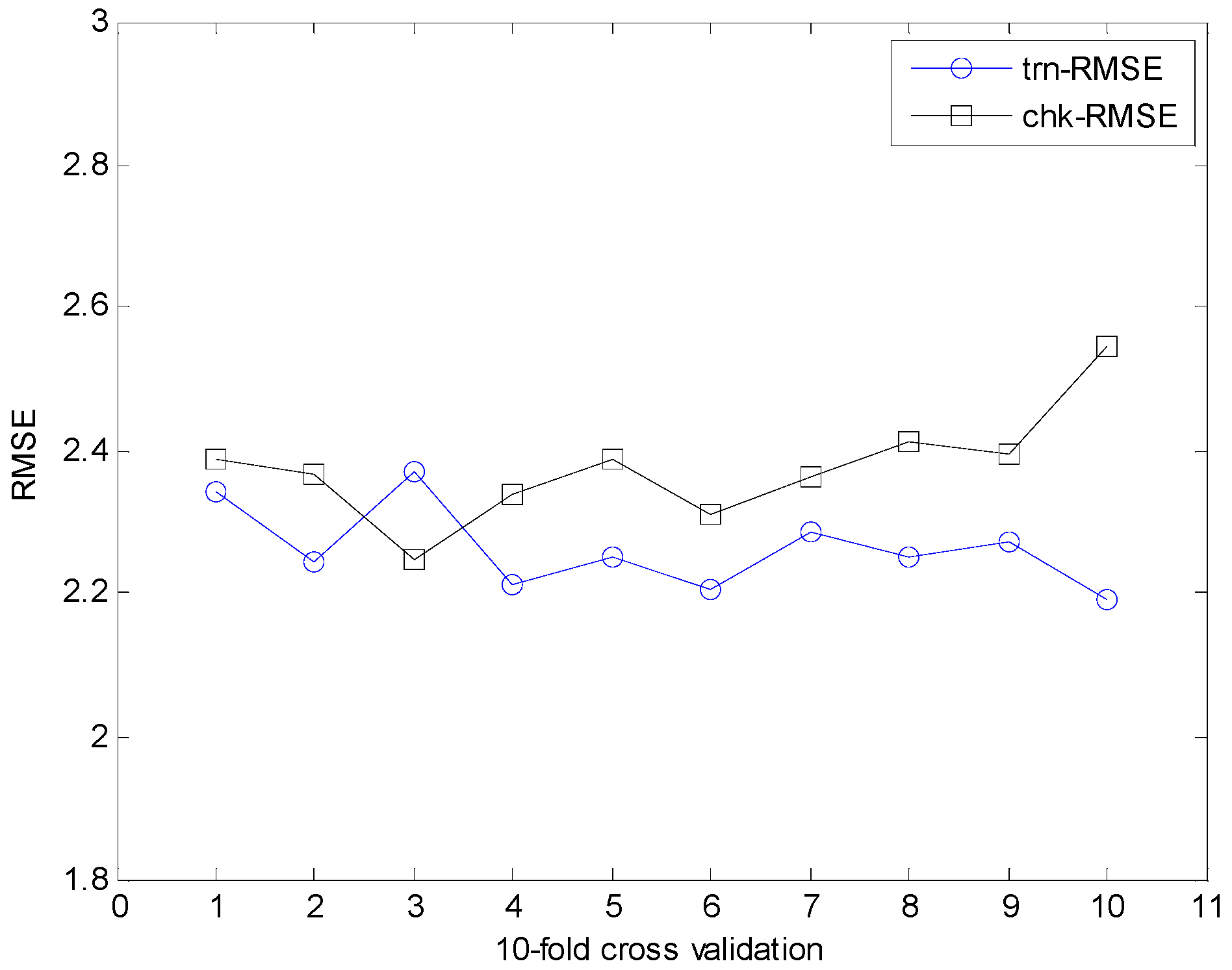
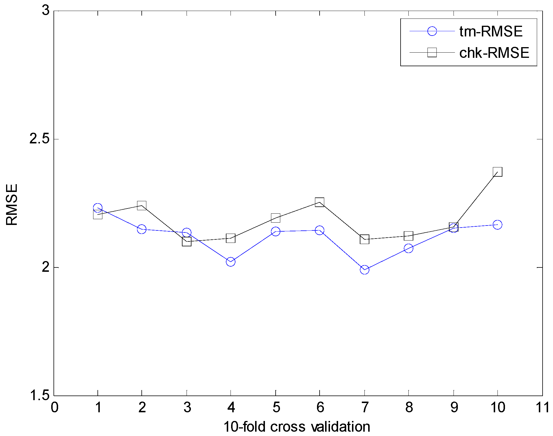
The energy analysis was obtained by twelve building shapes [23]. The dataset includes 768 data pairs and eight attributes. The output variables are the heating and cooling load with real-valued responses. Figure 13 and Figure 14 show the simulation results through ANFN and IANFN, respectively. Figure 15, Figure 16 and Figure 17 show the results of 10-fold cross validation for the proposed methods. Here trn-RMSE and chk-RMSE denote the RMSE value for the training and testing dataset in the case of heating load prediction, respectively. Table 2 lists the RMSE values for the proposed approach and the previous methods. It was found from the results that IIM outperformed the previous methods in the generalization capability. The simulation results demonstrated that the IIM is both effective and superior to previous approaches. In particular, the incremental methods outperformed the typical IM. However, IANFN + LR presented superiority in the approximation capability, although IANFN + QR presented superiority in the generalization capability.
The experiments on cooling load were performed in the same manner as for heating load prediction. Figure 18 shows the prediction using ANFN as a local granular network. Figure 19 shows the results for cooling load. Figure 20, Figure 21 and Figure 22 show the RMSE results for the proposed methods. Here, trn-RMSE and chk-RMSE denote the RMSE value in the case of cooling load prediction. Table 3 lists the performance comparison for cooling load. The IRBFN and IANFN with LR outperformed the previous methods, as well as IM itself. Furthermore, the experimental results demonstrated that the proposed methods outperformed LR, LM, CFCM-RBFN and IM itself.
4.3. Boston Housing Data and Computer Hardware Datasets
We performed the experiment with two selected datasets for the machine learning examples. Firstly, the Boston housing dataset deals with the problem of real estate price prediction. In this example, we used twelve input variables except for one binary attribute. The data include 506 data pairs. Next, the computer hardware dataset is related to the CPU performance. This data consist of 209 data pairs with eight attributes except for the vendor name. The output to be predicted is estimated relative performance. The experimental method was performed in the same manner as in Section 4.1 and Section 4.2. Table 4 and Table 5 list the comparison results of RMSE for the Boston housing and computer hardware dataset, respectively. To search for an appropriate IIM in terms of the best generalization capability, we tried different models with the number of clusters and contexts varying from 2–8. Here, the proposed IANFN achieved the best performance at the generalization capability. The IIM obviously outperformed the IRBFN and IANFN based on LR. In particular, the IIM with QR showed good approximation capability showing a big difference in performance due to strong the nonlinear characteristics of computer hardware data.
5. Conclusions
We developed two IMs (IRBFN and IANFN) based on IIM combined with QR. The simulation results demonstrated that both IIM types outperformed the various previous approaches. The proposed methods have the ability to construct powerful networks using the improved incremental models from only target system sample data. The integration of global and local network results in a new framework of computational intelligence. Because of its numerical computation, the proposed method can be applied to a number of new application domains. These application domains are mostly computationally intensive and include adaptive signal processing, adaptive control, nonlinear system modeling, nonlinear regression and pattern recognition.
Acknowledgments
This research was supported by the “Human Resources Program in Energy Technology” of the Korea Institute of Energy Technology Evaluation and Planning (KETEP). Financial resources were granted by the Ministry of Trade, Industry and Energy, Republic of Korea (No. 20174030201620).
Author Contributions
Chan-Uk Yeom suggested the idea of the work and performed the experiments. Keun-Chang Kwak designed the experimental method. Both authors wrote and critically revised the paper.
Conflicts of Interest
The authors declare no conflict of interest.
References
- Jang, J.S.R.; Sun, C.T.; Mizutani, E. Neuro-Fuzzy and Soft Computing: A Computational Approach to Learning and Machine Intelligence; Prentice Hall: New Dehli, India, 1997. [Google Scholar]
- Pedrycz, W.; Gomide, F. Fuzzy Systems Engineering: Toward Human-Centric Computing; IEEE Press: New York, NY, USA, 2007. [Google Scholar]
- Bezdek, J.C. Pattern Recognition with Fuzzy Objective Function Algorithms; Plenum Press: New York, NY, USA, 1981. [Google Scholar]
- Chiu, S.L. Fuzzy model identification based on cluster estimation. J. Intell. Fuzzy Syst. 1994, 2, 267–278. [Google Scholar]
- Gustafson, D.E.; Kessel, W.C. Fuzzy clustering with a fuzzy covariance matrix. In Proceedings of the Decision and Control Including 17th Symposium on Adaptive Processes, San Diego, CA, USA, 10–12 January 1978; pp. 761–766. [Google Scholar]
- Abonyi, J.; Babuska, R.; Szeifert, F. Modified Gath-Geva fuzzy clustering for identification of Takagi-Sugeno fuzzy models. IEEE Trans. Syst. Man Cybern. Part B 2002, 32, 612–621. [Google Scholar] [CrossRef] [PubMed]
- Wang, C.; Yu, J.; Yang, M.S. Analysis of parameter selection for Gustafson-Kessel fuzzy clustering using Jocobian matrix. IEEE Trans. Fuzzy Syst. 2015, 23, 2329–2342. [Google Scholar]
- Lin, K.P. A novel evolutionary kernel intuitionistic fuzzy c-means clustering algorithm. IEEE Trans. Fuzzy Syst. 2014, 22, 1074–1087. [Google Scholar] [CrossRef]
- Pedrycz, W.; Izakian, H. Cluster-centric fuzzy modeling. IEEE Trans. Fuzzy Syst. 2014, 22, 1585–1597. [Google Scholar] [CrossRef]
- Pedrycz, W. Conditional fuzzy C-Means. Pattern Recognit. Lett. 1996, 17, 625–632. [Google Scholar] [CrossRef]
- Pedrycz, W. Conditional fuzzy clustering in the design of radial basis function neural networks. IEEE Trans. Neural Netw. 1998, 9, 601–612. [Google Scholar] [CrossRef] [PubMed]
- Pedrycz, W.; Vasilakos, A.V. Linguistic models and linguistic modeling. IEEE Trans. Syst. Man Cybern. 1999, 29, 745–757. [Google Scholar] [CrossRef] [PubMed]
- Pedrycz, W.; Kwak, K.C. Linguistic models as a framework of user-centric system modeling. IEEE Trans. Syst. Man Cybern. Part A 2006, 36, 727–745. [Google Scholar] [CrossRef]
- Pedrycz, W.; Kwak, K.C. The development of incremental models. IEEE Trans. Fuzzy Syst. 2007, 15, 507–518. [Google Scholar] [CrossRef]
- Reyes-Galaviz, O.F.; Pedrycz, W. Granular fuzzy models: Analysis, design, and evaluation. Int. J. Approx. Reason. 2015, 64, 1–19. [Google Scholar] [CrossRef]
- Li, J.; Pedrycz, W.; Wang, X. A rule-based development of incremental models. Int. J. Approx. Reason. 2015, 64, 20–38. [Google Scholar] [CrossRef]
- Mamdani, E.H.; Assilian, S. An experiment in linguistic synthesis with a fuzzy logic controller. Int. Man Mach. Stud. 1975, 7, 1–13. [Google Scholar] [CrossRef]
- Kwak, K.C.; Kim, S.S. Development of quantum-based adaptive neuro-fuzzy networks. IEEE Trans. Syst. Man Cybern. Part B. 2010, 40, 91–100. [Google Scholar]
- Kwak, K.C. A design of incremental granular model using context-based interval type-2 fuzzy c-means clustering algorithm. IEICE Trans. Inf. Syst. 2016, E99-D, 309–312. [Google Scholar] [CrossRef]
- UCI Machine Learning Repository. Available online: https://archive.ics.uci.edu/ml/datasets (accessed on 2 November 2017).
- Lee, M.W.; Kwak, K.C.; Pedrycz, W. An expansion of local granular models in the design of incremental model. In Proceedings of the 2016 IEEE International Conference on Fuzzy Systems (FUZZ-IEEE), Vancouver, BC, Canada, 24–29 July 2016; pp. 1664–1670. [Google Scholar]
- Lee, M.W.; Kwak, K.C. An incremental radial basis function networks based on information granules and its application. Comput. Intell. Neurosci. 2016, 2016, 3207627. [Google Scholar] [CrossRef] [PubMed]
- Tsanas, A.; Xifara, A. Accurate quantitative estimation of energy performance of residential buildings using statistical machine learning tools. Energy Build. 2012, 49, 560–567. [Google Scholar] [CrossRef]
Figure 1.
The schematic understanding of the incremental model (IM).
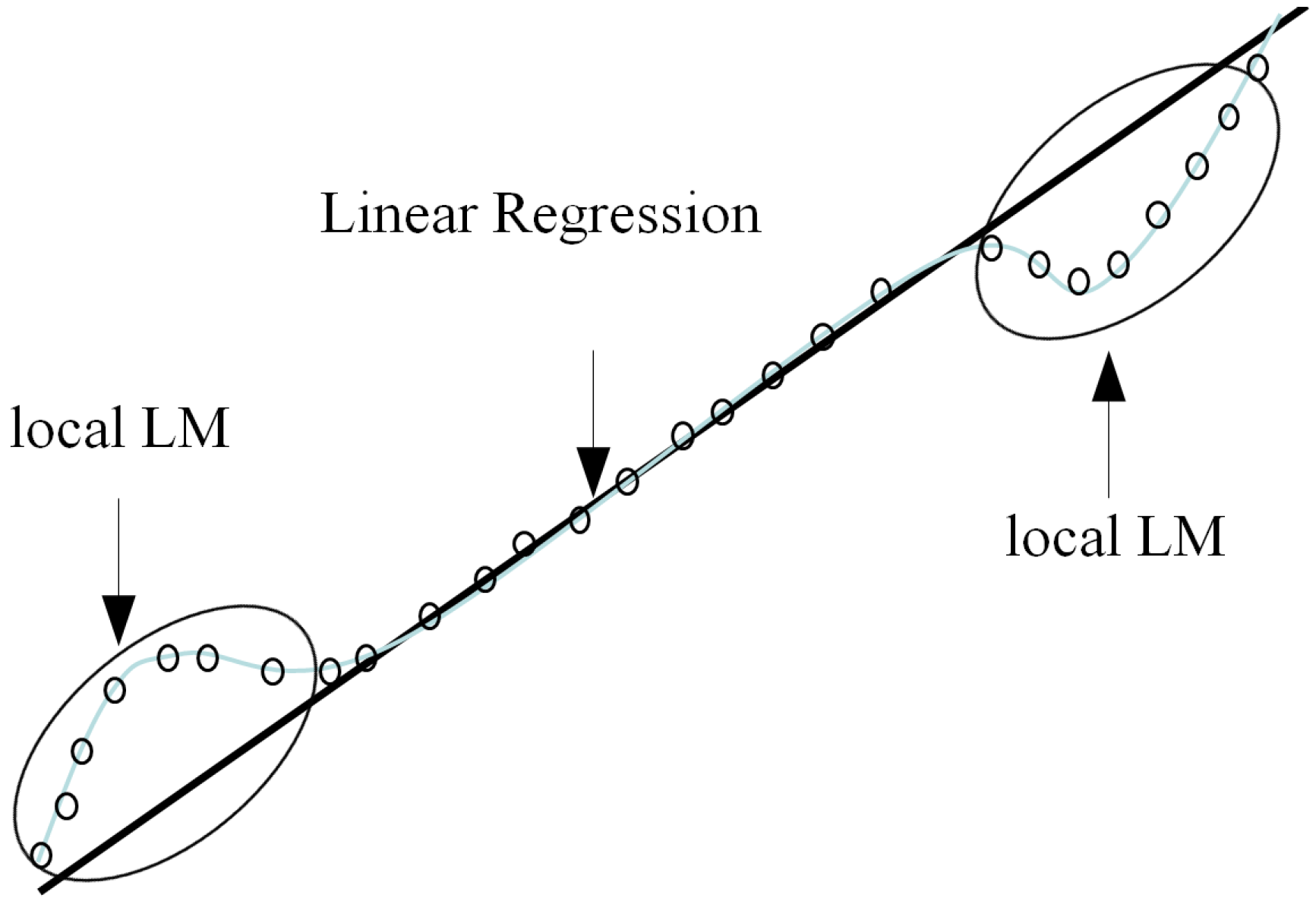
Figure 2.
Six contexts with linguistic labels. LR, linear regression.

Figure 3.
Architecture of IM based on LR and local Linguistic Model (LM).
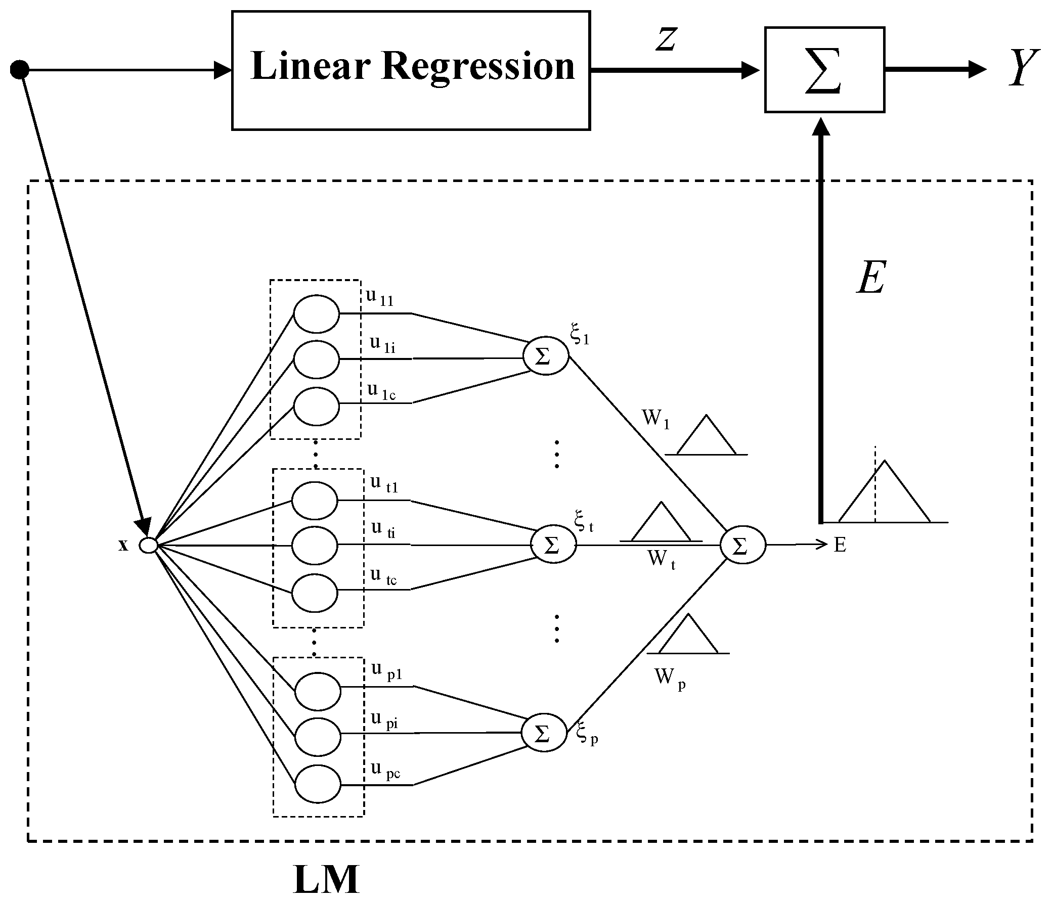
Figure 4.
The concept of improved IM (IIM) using QR and local granular networks.
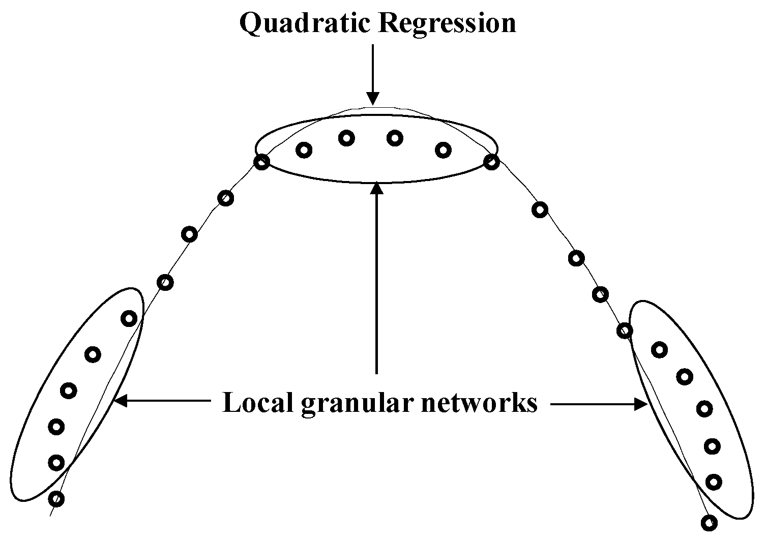
Figure 5.
Architecture of incremental radial basis function networks (IRBFN).
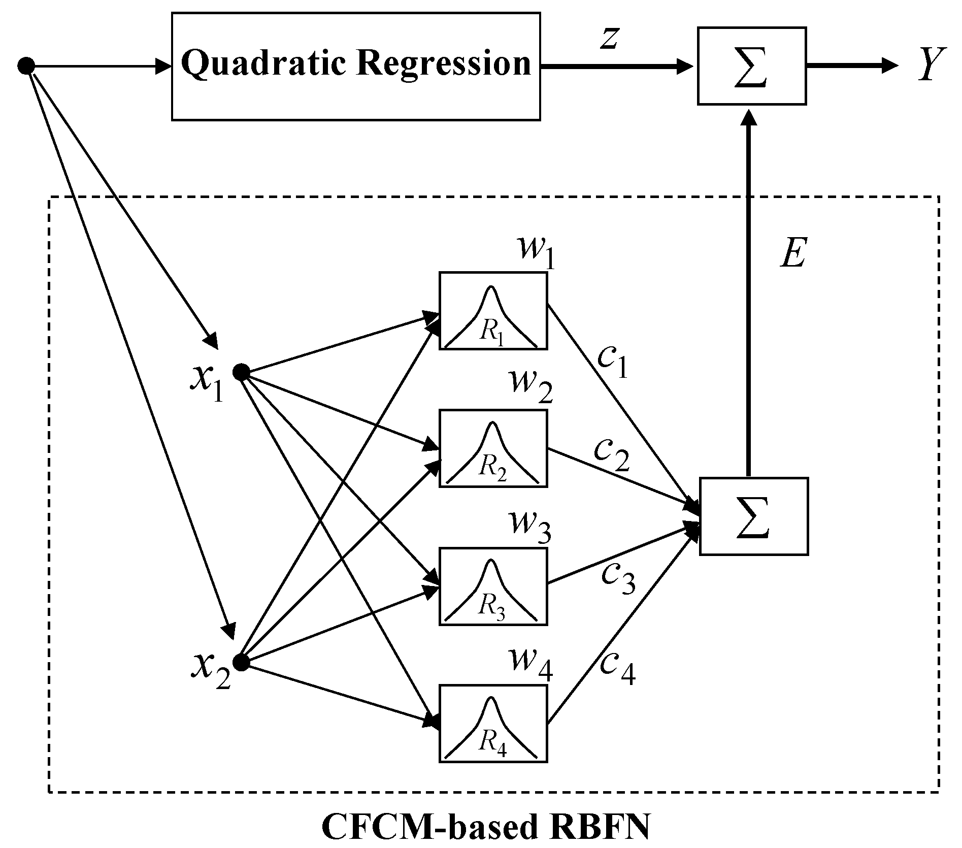
Figure 6.
Architecture of incremental adaptive neuro-fuzzy networks (IANFN).

Figure 7.
Schema of the proposed IANFN. QR, quadratic regression; TSK, Takagi–Sugeno–Kang.
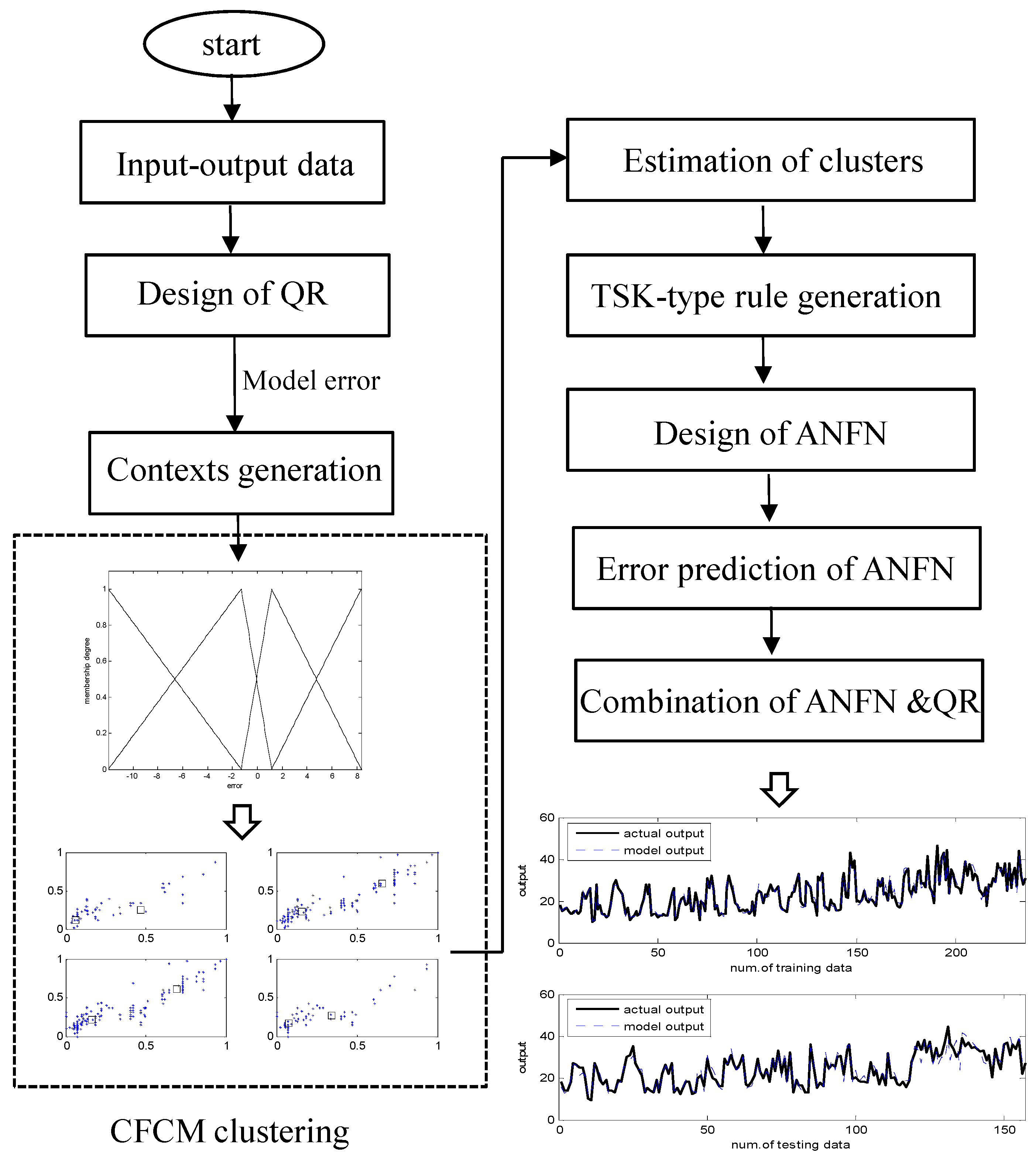
Figure 8.
Contexts produced by the error (number of contexts p = 6, IM).
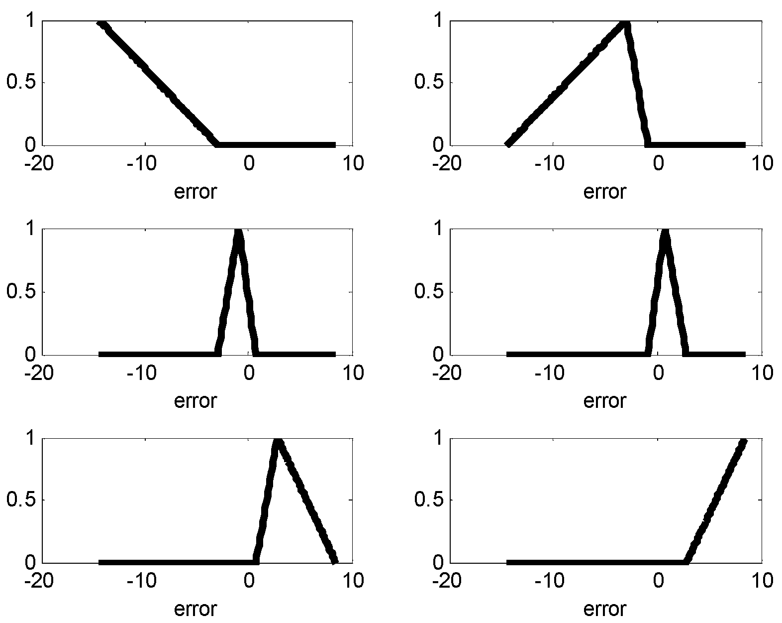
Figure 9.
Clusters generated in each context (c = 6).

Figure 10.
Contexts produced by the error (p = 4, IANFN).

Figure 11.
Cluster centers generated in each context (c = 2).

Figure 12.
Prediction of the proposed ANFN.
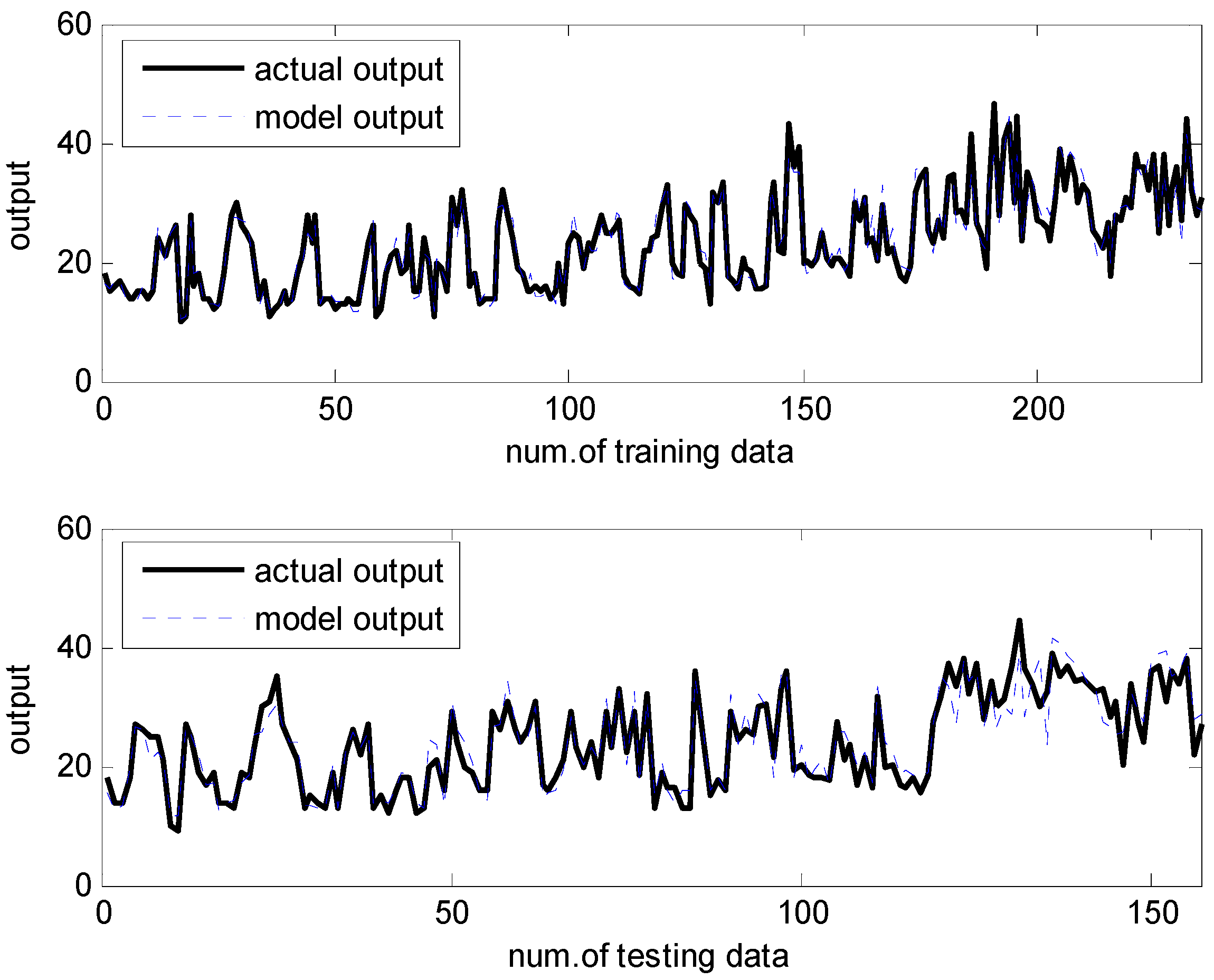
Figure 13.
Compensation by ANFN.

Figure 14.
IANFN result for heating load.
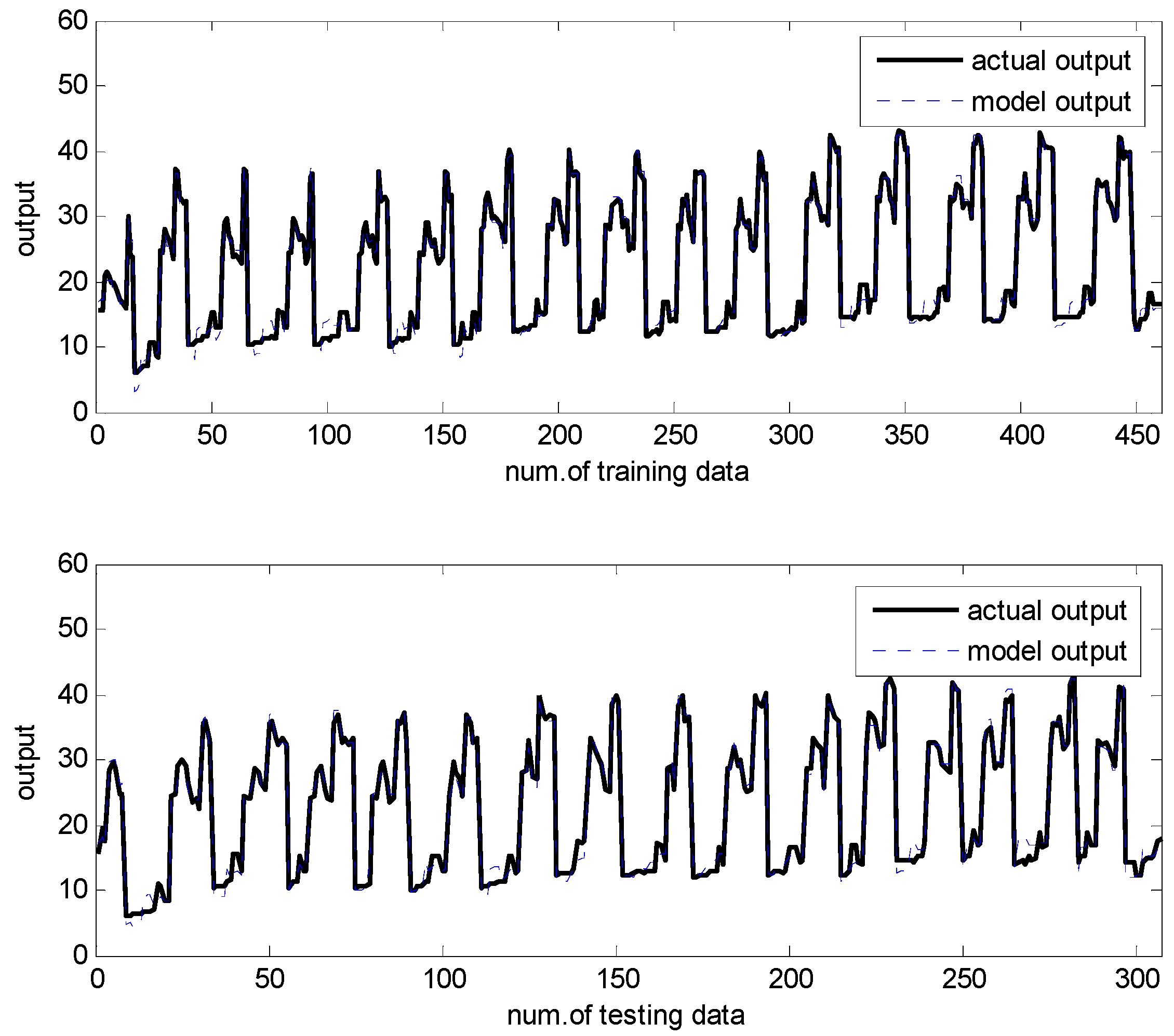
Figure 15.
Results of 10-fold cross validation for IRBFN-LSE (heating load).

Figure 16.
Results of 10-fold cross validation for IRBFN-BP (heating load).

Figure 17.
Results of 10-fold cross validation for IANFN (heating load).
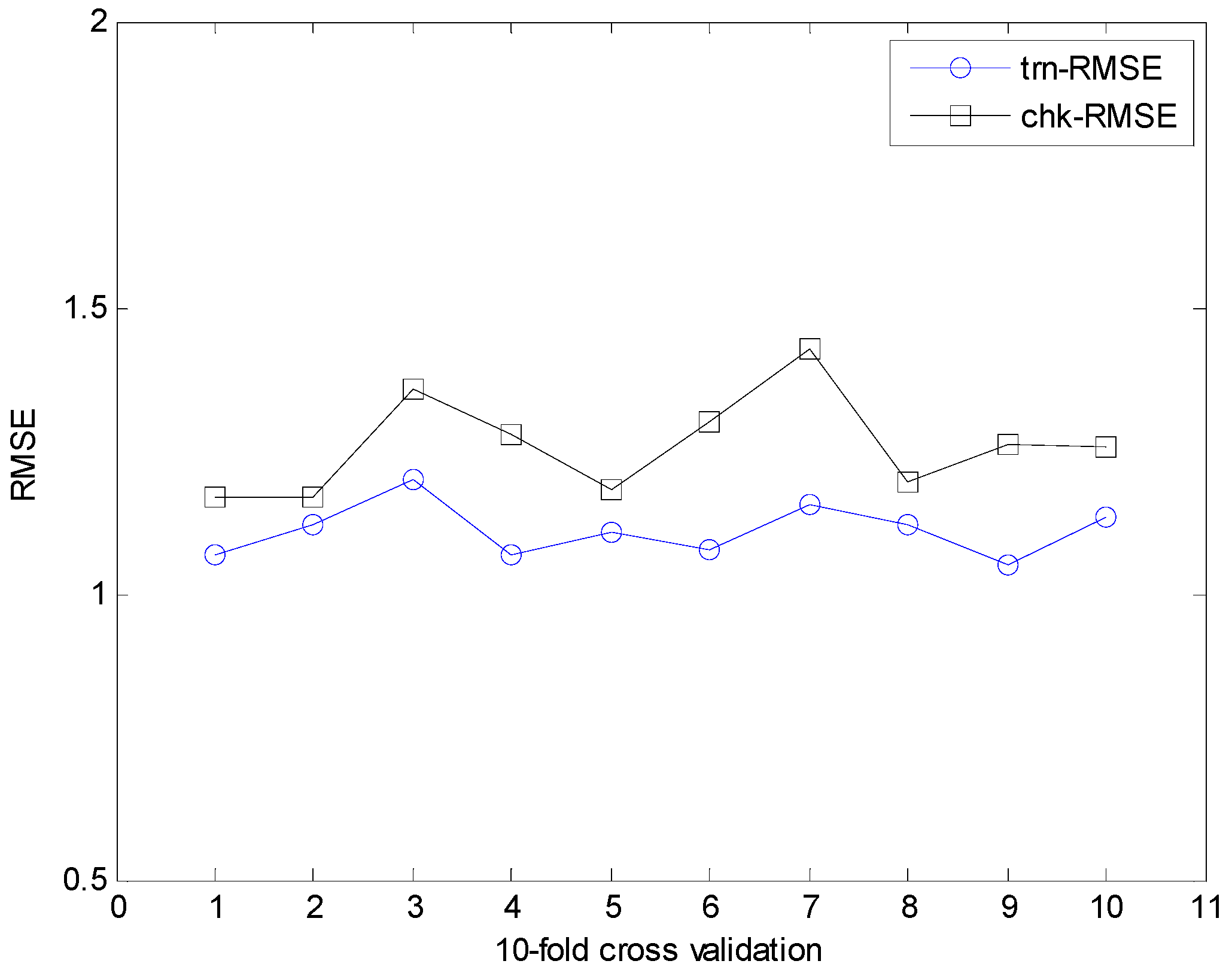
Figure 18.
Compensation by IANFN.

Figure 19.
IRBFN-LSE result for cooling load.
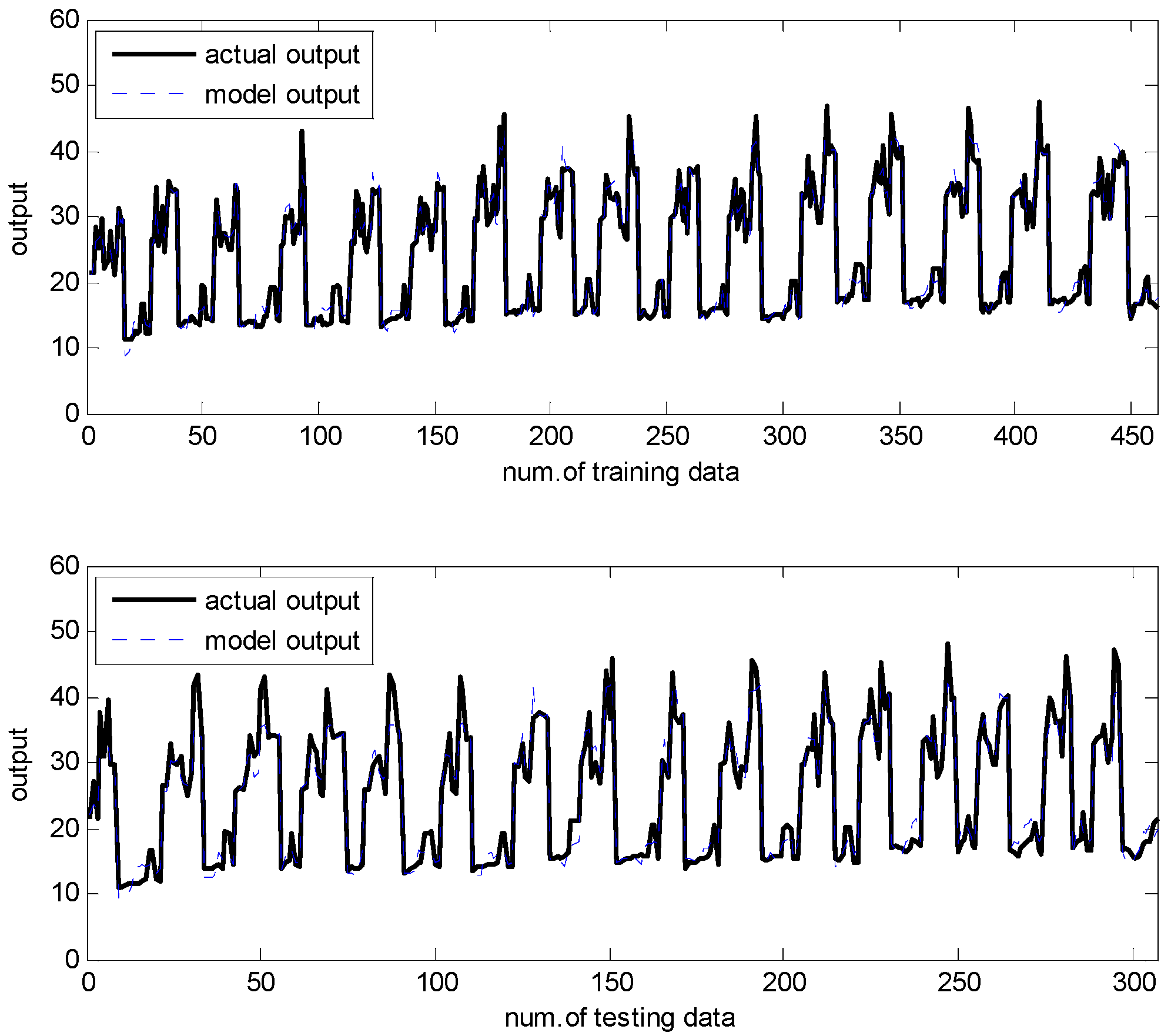
Figure 20.
10-fold cross validation for IRBFN-LSE (cooling load).
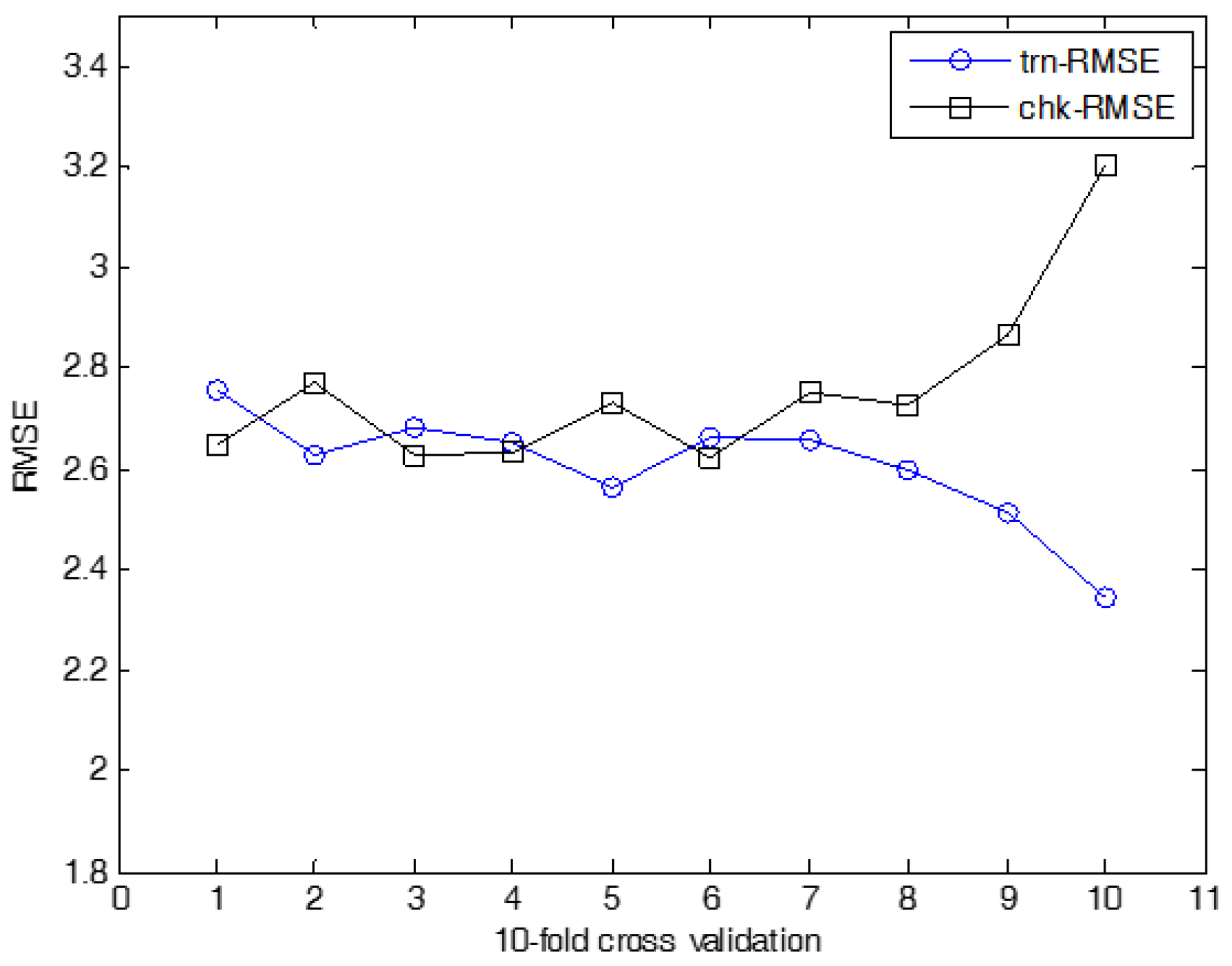
Figure 21.
10-fold cross validation for IRBFN-BP (cooling load).

Figure 22.
10-fold cross validation for IANFN (cooling load).

Table 1.
Performance comparison.
| Methods | No. of Rules | trn-RMSE | chk-RMSE | ||
|---|---|---|---|---|---|
| LR | - | 3.38 | 3.47 | ||
| LM [12] | 36 | 2.80 | 3.32 | ||
| RBFN (CFCM) [11] | 36 | 2.34 | 3.18 | ||
| IM [14] | 36 | 2.41 | 3.10 | ||
| IRBFN (LR) [21] | LSE | 36 | 2.03 | 3.04 | |
| BP | 36 | 2.62 | 2.92 | ||
| IANFN (LR) [21] | 8 | 2.10 | 2.74 | ||
| IIM | Proposed IRBFN | LSE | 9 | 1.74 | 2.63 |
| BP | 9 | 2.36 | 2.87 | ||
| Proposed IANFN | 8 | 2.05 | 2.46 | ||
Table 2.
Performance comparison.
| Methods | No. of Rules | trn-RMSE | chk-RMSE | ||
|---|---|---|---|---|---|
| LR | - | 2.94 | 2.91 | ||
| LM [12] | 36 | 3.70 | 4.02 | ||
| RBFN (CFCM) [11] | 36 | 2.77 | 3.11 | ||
| IM [14] | 36 | 2.46 | 2.80 | ||
| IRBFN (LR) [21] | LSE | 36 | 2.28 | 2.83 | |
| BP | 36 | 2.35 | 2.73 | ||
| IANFN (LR) [21] | 8 | 1.05 | 1.32 | ||
| IIM | Proposed IRBFN | LSE | 9 | 2.26 | 2.38 |
| BP | 9 | 2.12 | 2.19 | ||
| Proposed IANFN | 8 | 1.11 | 1.26 | ||
Table 3.
Performance comparison.
| Methods | No. of Rules | trn-RMSE | chk-RMSE | ||
|---|---|---|---|---|---|
| LR | - | 3.18 | 3.21 | ||
| LM [12] | 36 | 3.87 | 4.30 | ||
| RBFN (CFCM) [11] | 36 | 2.87 | 3.39 | ||
| IM [14] | 36 | 2.66 | 3.10 | ||
| IRBFN (LR) [21] | LSE | 36 | 2.46 | 3.10 | |
| BP | 36 | 2.56 | 3.09 | ||
| IANFN (LR) [21] | 8 | 1.93 | 2.38 | ||
| IIM | Proposed IRBFN | LSE | 9 | 2.61 | 2.76 |
| BP | 9 | 2.46 | 2.64 | ||
| Proposed IANFN | 8 | 1.858 | 2.153 | ||
© 2017 by the authors. Licensee MDPI, Basel, Switzerland. This article is an open access article distributed under the terms and conditions of the Creative Commons Attribution (CC BY) license (http://creativecommons.org/licenses/by/4.0/).
Share and Cite
MDPI and ACS Style
Yeom, C.-U.; Kwak, K.-C. The Development of Improved Incremental Models Using Local Granular Networks with Error Compensation. Symmetry 2017, 9, 266. https://doi.org/10.3390/sym9110266
AMA Style
Yeom C-U, Kwak K-C. The Development of Improved Incremental Models Using Local Granular Networks with Error Compensation. Symmetry. 2017; 9(11):266. https://doi.org/10.3390/sym9110266
Chicago/Turabian StyleYeom, Chan-Uk, and Keun-Chang Kwak. 2017. "The Development of Improved Incremental Models Using Local Granular Networks with Error Compensation" Symmetry 9, no. 11: 266. https://doi.org/10.3390/sym9110266
Note that from the first issue of 2016, this journal uses article numbers instead of page numbers. See further details here.