New Operations of Picture Fuzzy Relations and Fuzzy Comprehensive Evaluation


1
College of Information Engineering, Shanghai Maritime University, Shanghai 201306, China
2
School of Arts and Sciences, Shaanxi University of Science & Technology, Xi’an 710021, China
3
College of Arts and Sciences, Shanghai Maritime University, Shanghai 201306, China
*
Author to whom correspondence should be addressed.
Symmetry 2017, 9(11), 268; https://doi.org/10.3390/sym9110268
Submission received: 7 October 2017
/
Revised: 31 October 2017
/
Accepted: 2 November 2017
/
Published: 8 November 2017
Abstract
:In this paper, some new operations and basic properties of picture fuzzy relations are intensively studied. First, a new inclusion relation (called type-2 inclusion relation) of picture fuzzy relations is introduced, as well as the corresponding type-2 union, type-2 intersection and type-2 complement operations. Second, the notions of anti-reflexive kernel, symmetric kernel, reflexive closure and symmetric closure of a picture fuzzy relation are introduced and their properties are explored. Moreover, a new method to solve picture fuzzy comprehensive evaluation problems is proposed by defining the new composition operation of picture fuzzy relations, and the picture fuzzy comprehensive evaluation model is built. Finally, an application example (about investment risk) of picture fuzzy comprehensive evaluation is given, and the effective experiment results are obtained.
1. Introduction
We meet many concepts in our everyday life. Most of them are vague than precise, and uncertainty is a common research topic of many branches of science (economics, engineering, environment, management science, medical science, and so on). However, uncertainty is an unintelligible expression without a straightforward description, and many theories were established, such as probability theory, fuzzy set theory [1,2,3], intuitionistic fuzzy set theory [4], hesitant fuzzy set theory [5,6,7,8], soft set theory [9,10,11,12], rough set theory [13,14,15,16,17], granular computing [18,19,20,21,22,23,24,25,26,27], et al.
Although an intuitionistic fuzzy set has been successfully applied in different areas, but there are situations that cannot be represented by it in real life, such as voting, we may face human opinions involving more answers of the type: yes, abstain, no and refusal. Thus, in 2013, B. C. Cuong proposed a new concept named picture fuzzy sets (PFSs) [28,29,30], which is an extension of fuzzy sets and intuitionistic fuzzy sets. Picture fuzzy sets give three degrees of an element named degree of positive membership, degree of neutral membership and degree of negative membership, respectively. The picture fuzzy set solved the voting problem successfully, and is applied to clustering [31], fuzzy inference [32], and decision-making [33,34].
Relations are a suitable tool for describing correspondences between objects. Crisp relations have served well in mathematical theories. However, there are some problems that can’t be solved through classic relationships, such as the relationship of two objects being vague. Therefore, after the fuzzy set was defined, the definition of fuzzy relations was also proposed by Zadeh in paper [1] as an extension of classic relationship. Then, some scholars study it and used it widely in many fields, such as decision making, clustering analysis [35,36,37,38], fuzzy comprehensive evaluation [39,40,41] and so on. Fuzzy relations can model vagueness; however, they cannot model uncertainty: there is no means to attribute reliability information to the membership degrees. Intuitionistic fuzzy sets, as defined by Atanassov [4], gave us a way to incorporate uncertainty in an additional degree. Burillo and Bustince gave the definition of intuitionistic fuzzy relations [42,43] and discussed some properties of them. Intuitionistic fuzzy relations are intuitionistic fuzzy sets in a Cartesian product of universes. In 2005, Lei et al. further researched intuitionistic fuzzy relations and composition operation of intuitionistic fuzzy relations [44]. Yang proposed the definition of kernels and closures of intuitionistic fuzzy relations and proved fourteen theorems of intuitionistic fuzzy relations [45]. B. C. Cuong proposed the notion of picture fuzzy relations and studied their operations and properties [28,29].
The rest of this paper is structured as follows. In Section 2, some basic notions and operations of picture fuzzy sets and picture fuzzy relations are provided. In Section 3, type-2 union, type-2 intersection, and type-2 complement operations of picture fuzzy relations are well described and their properties are studied. In Section 4 and Section 5, kernels and closures of a picture fuzzy relation are discussed. Their computational formulas and some properties are also obtained. Meanwhile, some examples are given. In Section 6, a new composition operation of picture fuzzy relations is investigated. Furthermore, according to the new composition operation, a new method to solve picture fuzzy comprehensive evaluation problems is proposed, and we also prove that this method is doable by an application example. The last section summarizes the conclusions.
2. Preliminary
2.1. Some Basic Concepts
In this section, several basic concepts and operations about picture fuzzy sets and picture fuzzy relations are provided.
Definition 1.
An intuitionistic fuzzy set (IFS) A on the universe X is an object of the form A = {(x, μA(x), νA(x)) | x ∈ X}, where μA(x) ∈ [0, 1] is called the “degree of membership of x in A”, νA(x) ∈ [0, 1] is called the “degree of non-membership of x in A”, and where μA(x) and νA(x) satisfy μA(x) + νA(x) ≤ 1 for all x ∈ X. In this paper, let IFS(X) denote the sets of all the intuitionistic fuzzy sets on X [4].
Definition 2.
A picture fuzzy set A on the universe X is an object of the form
where μA(x) ∈ [0, 1] is called the “degree of positive membership of x in A”, ηA(x) ∈ [0, 1] is called the “degree of neutral membership of x in A”, and νA(x) ∈ [0, 1] is called the “degree of negative membership of x in A”, and μA(x), ηA(x), νA(x) satisfy μA(x) + ηA(x) + νA(x) ≤ 1, for all x ∈ X. Then, ∀ x ∈ X, 1 − (μA(x) + ηA(x) + νA(x)) is called the “degree of refusal membership of x in A”. Let PFS(X) denote the set of all the picture fuzzy sets on a universe X [28].
Definition 3.
A picture fuzzy relation is a picture fuzzy subset of X × Y i.e., R given by
where μR: X × Y → [0, 1], ηR: X × Y → [0, 1], and νR: X × Y → [0, 1] satisfy the condition 0 ≤ μR(x, y) + ηR(x, y) + νR(x, y) ≤ 1, for every (x, y) ∈ X × Y. PFR(X × Y) the set of all the picture fuzzy relations in X × Y is denoted [29].
R = {((x, y), μR(x, y), ηR(x, y), νR(x, y))|x ∈ X, y ∈ Y},
Definition 4.
Let R ∈ PFR(X × Y). We define the inverse relation R−1 between Y and X: μR−1(y, x) = μR(x, y), ηR−1(y, x) = ηR(x, y), νR−1(y, x) = νR(x, y), ∀ (x, y) ∈ X × Y [29].
Definition 5.
Let R and P be two picture fuzzy relations between X and Y, for every (x, y) ∈ X × Y we define [29]:
- (1)
- R ⊆ P iff μR(x, y) ≤ μP(x, y), ηR(x, y) ≤ ηP(x, y), νR(x, y) ≥ νP(x, y);
- (2)
- R ∪ P = {((x, y), μR(x, y) ∨ μP(x, y), ηR(x, y) ∧ ηP(x, y), νR(x, y) ∧ νP(x, y)) | x ∈ X, y ∈ Y};
- (3)
- R ∩ P = {((x, y), μR(x, y) ∧ μP(x, y), ηR(x, y) ∧ ηP(x, y), νR(x, y) ∨ νP(x, y)) | x ∈ X, y ∈ Y};
- (4)
- Rc = {((x, y), νR(x, y), ηR(x, y), μR(x, y)) | x ∈ X, y ∈ Y}.
Proposition 1.
- (a) (R−1)−1 = R;
- (b) R ⊆ P ⇒ R−1 ⊆ P−1;
- (c1) (R ∪ P)−1 = R−1 ∪ P−1;
- (c2) (R ∩ P)−1 = R−1 ∩ P−1;
- (d1) R ∩ (P ∪ Q) = (R ∩ P) ∪ (R ∩ Q);
- (d2) R ∪ (P ∩ Q) = (R ∪ P) ∩ (R ∪ Q);
- (e) R ∩ P ⊆ R, R ∩ P ⊆ P;
- (f1) If (R ⊇ P) and (R ⊇ Q), then R ⊇ P ∪ Q;
- (f2) If (R ⊆ P) and (R ⊆ Q), then R ⊆ P ∩ Q.
Definition 6.
Let E ∈ PFR(X × Y) and P ∈ PFR(Y × Z). Max-min composed relation PCE ∈ PFR(X × Z) is called to the one defined by [29]:
where ∀ (x, z) ∈ X × Z:
PCE = {((x, z), μPCE(x, z), ηPCE(x, z), νPCE(x, z))|x ∈ X, z ∈ Z},
Definition 7.
Let α = (μα, ηα, να, ρα) be a picture fuzzy number, μα + ηα + να ≤ 1, ρα = 1 − μα − ηα − να. The score function S can be defined as S(α) = μα − να, and the accuracy function H is given by H(α) = μα + ηα + να, which S(α) ∈ [−1, 1], H(α) ∈ [0, 1]. Then, for two picture fuzzy numbers α and β [33],
- (1)
- if S(α) > S(β), then α is superior to β, denoted by α ⊱ β;
- (2)
- if S(α) = S(β), then
- (i)
- if H(α) = H(β), implies that α is equivalent to β, denoted by α ~ β;
- (ii)
- if H(α) > H(β), implied that α is superior to β, denoted by α ⊱ β.
We also use voting as a good example to explain the above definition, where S(α) = μα − να represents goal difference and H(α) = μα + ηα + να can be interpreted as the effective degree of voting. When S(α) increases, we can know that there are more people who vote for α and people who vote against α become less. When H(α) increases, we can know that there are more people who vote for or against α and people who refuse to vote become less. Therefore, H(α) depicts the effective degree of voting.
2.2. On Inclusion Relation of Picture Fuzzy Relations
From now on, we will assume that if x, y ∈ D*, then x1, x2 and x3 denote, respectively, the first, the second and the third component of x, i.e., x = (x1, x2, x3). We denote the units of D* by 1D* = (1, 0, 0) and 0D* = (0, 0, 1), respectively.
Obviously, for every picture fuzzy set:
It corresponds with a D*-fuzzy set, i.e., a mapping:
The original inclusion relation of picture fuzzy relations is based on the following order relation on D*: ∀ x, y ∈ D*,
The above “∧“ denote “and”. In this paper, above “≤1” is called type-1 order relation and the original inclusion relation of picture fuzzy relations is called a type-1 inclusion relation, and denoted as the following:
R ⊆1 P iff (∀ (x, y) ∈ X × Y, μR(x, y) ≤ μP(x, y), ηR(x, y) ≤ ηP(x, y), νR(x, y) ≥ νP(x, y)).
Accordingly, the union, intersection and complement operations in Definition 5 are called type-1 union, intersection and complement, and denoted as the following:
R ∪1 P = {((x, y), μR(x, y) ∨ μP(x, y), ηR(x, y) ∧ ηP(x, y), νR(x, y) ∧ νP(x, y)) | x ∈ X, y ∈ Y}
= {((x, y), (μR(x, y), ηR(x, y), νR(x, y)) ∨1 (μP(x, y), ηP(x, y), νP(x, y))) | x ∈ X, y ∈ Y};
= {((x, y), (μR(x, y), ηR(x, y), νR(x, y)) ∨1 (μP(x, y), ηP(x, y), νP(x, y))) | x ∈ X, y ∈ Y};
R ∩1 P = {((x, y), μR(x, y) ∧ μP(x, y), ηR(x, y) ∧ ηP(x, y), νR(x, y) ∨ νP(x, y))} | x ∈ X, y ∈ Y}
= {((x, y), (μR(x, y), ηR(x, y), νR(x, y)) ∧1 (μP(x, y), ηP(x, y), νP(x, y))) | x ∈ X, y ∈ Y};
= {((x, y), (μR(x, y), ηR(x, y), νR(x, y)) ∧1 (μP(x, y), ηP(x, y), νP(x, y))) | x ∈ X, y ∈ Y};
Rc1 = {((x, y), νR(x, y), ηR(x, y), μR(x, y)) | x ∈ X, y ∈ Y} = {((x, y), (μR(x, y), ηR(x, y), νR(x, y))c1) | x ∈ X, y ∈ Y}.
Now, we introduce a new inclusion of picture fuzzy relations, and call it type-2 inclusion of picture fuzzy relations.
Definition 8.
Let R and P be two picture fuzzy relations between X and Y. The type-2 inclusion relation is defined as follows: R ⊆2 P if and only if ∀ (x, y) ∈ X × Y, (μR(x, y) < μP(x, y), νR(x, y) ≥ νP(x, y)), or (μR(x, y) = μP(x, y), νR(x, y) > νP(x, y)), or (μR(x, y) = μP(x, y), νR(x, y) = νP(x, y) and ηR(x, y) ≤ ηP(x, y)).
In fact, type-2 inclusion relation is based on the following order relation on D* (see [5], and it is called a type-2 order relation in this paper):
The above “∧“ denote “and”, “∨“ denote “or”.
Remark 1.
In order not to cause confusion, the type-2 order relation on D* is denoted by “≤2”, it is different from [30].
Note that, if for any x, y ∈ D* that neither x ≤2 y nor y ≤2 x, then x and y are incomparable, denoted as
3. New Operations and Properties of Picture Fuzzy Relations
In this section, we introduce some new operations named type-2 inclusion, type-2 union, type-2 intersection and type-2 complement operation of picture fuzzy relations and study their properties.
For any picture fuzzy relations R and P on X × Y, by Definition 8, we have:
R ⊆2 P if and only if ∀ (x, y) ∈ X × Y, (μR(x, y), ηR(x, y), νR(x, y)) ≤2 (μP(x, y), ηP(x, y), νP(x, y)).
From this, we can get the following proposition.
Proposition 2.
Let R, P and Q be picture fuzzy relations on X × Y, then
- (1)
- R ⊆2 R;
- (2)
- (R ⊆2 P, P ⊆2 R) ⇒ R = P;
- (3)
- (R ⊆2 P, P ⊆2 Q) ⇒ R ⊆2 Q.
Definition 9.
For every two PFRs R and P, the type-2 union, type-2 intersection, type-2 complement operators are defined as follows:
- (1)
- R ∪2 P =
- (2)
- R ∩2 P =
- (3)
- co(R) = Rc2 =
It is easy to verify that the type-2 union and type-2 intersection of PFRs satisfy commutative law and associative law.
Example 1.
Definition 10.
Let R ∈ PFR(X × Y).
- (1)
- If ∀ (x, y) ∈ X × Y, μR(x, y) = ηR(x, y) = 0 and νR(x, y) = 1, then R is called a null PFR, denoted by ∅N.
- (2)
- If ∀ (x, y) ∈ X × Y, μR(x, y) = 1 and ηR(x, y) = νR(x, y) = 0, then R is called an absolute PFR, denoted by UN.
- (3)
- If ∀ (x, y) ∈ X × Y, μR(x, y) = , ηR(x, y) = 0 and νR(x, y) = , then R is called an identity PFR, denoted by IdN.
According the Definitions 9 and 10, we can get the Type-2 complement of IdN denoted by (IdN)c2 is a PFR satisfying: ∀ (x, y) ∈ X × Y,
Definition 11.
Let R ∈ PFR(X × Y).
- (1)
- If ∀ x ∈ X, μR(x, x) = 1 and ηR(x, x) = νR(x, x) = 0, then R is called a reflexive PFR.
- (2)
- If ∀ (x, y) ∈ X × Y, μR(x, y) = μR(y, x), ηR(x, y) = ηR(y, x), νR(x, y) = νR(y, x), then R is called a symmetric PFR.
- (3)
- If ∀ x ∈ X, μR(x, x) = ηR(x, x) = 0 and νR(x, x) = 1, then R is called an anti-reflexive PFR.
Proposition 3.
Type-2 union and type-2 intersection of PFRs don’t satisfy distributive law, which means that ∀ R, P, Q ∈ PFR(X × Y):
- (1)
- (R ∩2 P) ∪2 Q ≠ (R ∪2 Q) ∩2 (P ∪2 Q),
- (2)
- (R ∪2 P) ∩2 Q ≠ (R ∩2 Q) ∪2 (P ∩2 Q).
Example 2.
X = {x1, x2}, Y = {y1, y2}. Picture fuzzy relations R, P, Q in X × Y are given in Table 1, Table 4 and Table 5. Then (R ∩2 P) ∪2 Q, (R ∪2 Q) ∩2 (P ∪2 Q), (R ∪2 P) ∩2 Q, (R ∩2 Q) ∪2 (P ∩2 Q) in X × Y are given in Table 6, Table 7, Table 8 and Table 9. Furthermore, according to Table 6, Table 7, Table 8 and Table 9, we can get the conclusion of Propositions 3 (1) and (2).
Proposition 4.
Let R, P, Q ∈ PFR(X × Y). Then, we have
- (1)
- R is symmetric iff R = R−1;
- (2)
- (Rc2)−1 = (R−1)c2;
- (3)
- (Rc2)c2 = R, (R−1)−1 = R;
- (4)
- R ⊆2 R ∪2 P, P ⊆2 R ∪2 P;
- (5)
- R ∩2 P ⊆2 R, R ∩2 P ⊆2 P;
- (6)
- If R ⊆2 P, then R−1 ⊆2 P−1;
- (7)
- If R ⊆2 P and Q ⊆2 P, then R ∪2 Q ⊆2 P;
- (8)
- If P ⊆2 R and P ⊆2 Q, then P ⊆2 R ∩2 Q;
- (9)
- If R ⊆2 P, then R ∪2 P = P, R ∩2 P = R;
- (10)
- (R ∪2 P)−1 = R−1 ∪2 P−1, (R ∩2 P)−1 = R−1 ∩2 P−1;
- (11)
- (R ∪2 P)c2 = Rc2 ∩2 Pc2, (R ∩2 P)c2 = Rc2 ∪2 Pc2.
Proof.
Clearly, Labels (1) and (3)–(9) is hold. We only show Labels (2), (10) and (11).
(2) ∀ (x, y) ∈ X × Y, μ(Rc2)−1(x, y) = μRc2(y, x) = νR(y, x) = νR−1(x, y) = μ(R−1)c2(x, y); ν(Rc2)−1(x, y) = νRc2(y, x) = μR(y, x) = μR−1(x, y) = ν(R−1)c2(x, y); η(Rc2)−1(x, y) = ηRc2(y, x) = 1 − μR(y, x) − ηR(y, x) − νR(y, x) = 1 − μR−1(x, y) − ηR−1(x, y) − νR−1(x, y) = η(R−1)c2(x, y).
Therefore (Rc2)−1 = (R−1)c2.
(10) If R ⊆2 P, then R−1 ⊆2 P−1, so (R ∪2 P)−1 = P−1 = R−1 ∪2 P−1; If P ⊆2 R, then P−1 ⊆2 R−1, so (R ∪2 P)−1 = R−1 = R−1 ∪2 P−1; If neither R ⊆2 P nor P ⊆2 R, then (R ∪2 P)−1 = {((x, y), μR(x, y) ∨ μP(x, y), 0, νR(x, y) ∧ νP(x, y)) | (x, y) ∈ X × Y }−1 = {((y, x), μR−1(x, y) ∨ μP−1(x, y), 0, νR−1(x, y) ∧ νP−1(x, y)) | (x, y) ∈ X × Y }, R −1 ∪2 P −1 = {((y, x), μR−1(x, y), ηR−1(x, y), νR−1(x, y)) | (x, y) ∈ X × Y } ∪2 {((y, x), μP−1(x, y), ηP−1(x, y), νP−1(x, y)) | (x, y) ∈ X × Y } = {((y, x), μR−1(x, y) ∨ μP−1(x, y), 0, νR−1(x, y) ∧ νP−1(x, y)) | (x, y) ∈ X × Y } = (R ∪2 P)−1. Hence, (R ∪2 P)−1 = R−1 ∪2 P−1. Similarly, we can show (R ∩2 P)−1 = R−1 ∩2 P−1.
(11) If R ⊆2 P, then Pc2 ⊆2 Rc2, so (R ∪2 P)c2 = Pc2 = Rc2 ∩2 Pc2; If P ⊆2 R, then Rc2 ⊆2 Pc2, so (R ∪2 P)c2 = Rc2 = Rc2 ∩2 Pc2; If neither R ⊆2 P nor P ⊆2 R, then neither Rc2 ⊆2 Pc2 nor Pc2 ⊆2 Rc2 and (R ∪2 P)c2 = {((x, y), νR(x, y) ∧ νP(x, y), 1 – (μR(x, y) ∨ μP(x, y)) – (νR(x, y) ∧ νP(x, y)), μR(x, y) ∨ μP(x, y)) | (x, y) ∈ X × Y }, Rc2 ∩2 Pc2 = {((x, y), νR(x, y), 1 – μR(x, y) – ηR(x, y) – νR(x, y), μR(x, y)) | (x, y) ∈ X × Y } ∩2 {((x, y), νP(x, y), 1 – μP(x, y) – ηP(x, y) – νP(x, y), μP(x, y)) | (x, y) ∈ X × Y } = {((x, y), νR(x, y) ∧ νP(x, y), 1 – (μR(x, y) ∨ μP(x, y)) – (νR(x, y) ∧ νP(x, y)), μR(x, y) ∨ μP(x, y)) | (x, y) ∈ X × Y }. Hence, (R ∪2 P)c2 = Rc2 ∩2 Pc2. Similarly, we can get (R ∩2 P)c2 = Rc2 ∪2 Pc2. ☐
4. Kernels of Picture Fuzzy Relations
In this section, we will give the definition of anti-reflexive kernel and symmetric kernel about a PFR, and then study their properties.
Definition 12.
Let R ∈ PFR(X × Y).
- (1)
- The maximal anti-reflexive PFR contained in R is called anti-reflexive kernel of R, denoted by ar(R).
- (2)
- The maximal symmetric PFR contained in R is called symmetric kernel of R, denoted by s(R).
Proposition 5.
Let R ∈ PFR(X × Y). Then,
- (1)
- ar(R) = R ∩2 (IdN)c2.
- (2)
- s(R) = R ∩2 R−1.
Proof.
(1) By Proposition 3 (5), R ∩2 (IdN)c2 ⊆2 R. According the definition of IdN, ∀ x ∈ X, we have μIdN(x, x) = 1 and ηIdN(x, x) = νIdN(x, x) = 0, then μ(IdN)c2(x, x) = η(IdN)c2(x, x) = 0 and ν(IdN)c2(x, x) = 1. Hence, μ(IdN)c2(x, x) ≤ μR(x, x), ν(IdN)c2(x, x) ≥ νR(x, x), η(IdN)c2(x, x) ≤ ηR(x, x). Therefore, (IdN)c2 ⊆2 R, μR∩2(IdN)c2(x, x) = ηR∩2(IdN)c2(x, x) = 0 and νR∩2(IdN)c2(x, x) = 1. According to Definition 11 (3), R ∩2 (IdN)c2 is an anti-reflexive PFR.
Suppose P is an anti-reflexive PFR and P ⊆2 R. Obviously, P ⊆2 (IdN)c2. Hence, P ⊆2 R ∩2 (IdN)c2. Therefore, ar(R) = R ∩2 (IdN)c2.
(2) By Proposition 3 (3) and Label (10), (R ∩2 R−1)−1 = R−1 ∩2 (R−1)−1 = R−1 ∩2 R = R ∩2 R−1, which implies that R ∩2 R−1 is a symmetric PFR. According to Proposition 3 (5), R ∩2 R−1 ⊆2 R.
Suppose P is a symmetric PFR and P ⊆2 R. By Proposition 3 (6), P−1 ⊆2 R−1. Then, by Proposition 3 (1) and (5), P = P−1 ⊆2 R ∩2 R−1. Therefore, s(R) = R ∩2 R−1. ☐
Example 3.
Proposition 6.
The anti-reflexive kernel operator ar of the PFR has the following properties:
- (1)
- ar(∅N) = ∅N, ar((IdN)c2) = (IdN)c2;
- (2)
- ∀ R ∈ PFR(X × Y), ar(R) ⊆2 R;
- (3)
- ∀ R, P ∈ PFR(X × Y), ar(R ∪2 P) = ar(R) ∪2 ar(P), ar(R ∩2 P) = ar(R) ∩2 ar(P);
- (4)
- ∀ R, P ∈ PFR(X × Y), if R ⊆2 P, then ar(R) ⊆2 ar(P);
- (5)
- ∀ R ∈ PFR(X × Y), ar(ar(R)) = ar(R).
Proof.
(1) By the definition of ∅N, we can get ∅N ⊆2 (IdN)c2. Therefore, ar(∅N) = ∅N ∩2 (IdN)c2 = ∅N. ar((IdN)c2) = (IdN)c2 ∩2 (IdN)c2 = (IdN)c2.
(2) ∀ R ∈ PFR(X × Y), by Proposition 5 (1) and Proposition 3 (5), ar(R) = R ∩2 (IdN)c2 ⊆2 R.
(3) ar(R ∪2 P) = (R ∪2 P) ∩2 (IdN)c2, ar(R) ∪2 ar(P) = (R ∩2 (IdN)c2) ∪2 (P ∩2 (IdN)c2). ∀ (x, y) ∈ X × Y, when x = y, (IdN)c2 = {((x, y), 0, 0, 1) | (x, y) ∈ X × Y }, so (IdN)c2 ⊆2 R, (IdN)c2 ⊆2 P, then ar(R ∪2 P) = ar(R) ∪2 ar(P) = (IdN)c2; when x ≠ y, (IdN)c2 = {((x, y), 1, 0, 0) | (x, y) ∈ X × Y }, so R ⊆2 (IdN)c2, P ⊆2 (IdN)c2, then ar(R ∪2 P) = ar(R) ∪2 ar(P) = R ∪2 P. Hence, ar(R ∪2 P) = ar(R) ∪2 ar(P). ar(R ∩2 P) = (R ∩2 P) ∩2 (IdN)c2 = ((R ∩2 (IdN)c2) ∩2 (P ∩2 (IdN)c2) = ar(R) ∩2 ar(P).
(4) ∀ R, P ∈ PFR(X × Y), if R ⊆2 P, by Label (3) and Proposition 3 (4) and Label (9), ar(R) ⊆2 ar(R) ∪2 ar(P) = ar(R ∪2 P) = ar(P).
(5) ∀ R ∈ PFR(X × Y), by Proposition 5 (1), ar(R) = R ∩2 (IdN)c2. Hence, ar(ar(R)) = ar(R ∩2 (IdN)c2) = (R ∩2 (IdN)c2) ∩2 (IdN)c2 = R ∩2 (IdN)c2 = ar(R). ☐
Proposition 7.
The symmetric kernel operator s of the PFR has the following properties:
- (1)
- s(∅N) = ∅N, s(UN) = UN, s(IdN) = IdN;
- (2)
- ∀ R ∈ PFR(X × Y), s(R) ⊆2 R;
- (3)
- ∀ R, P ∈ PFR(X × Y), s(R ∩2 P) = s(R) ∩2 s(P);
- (4)
- ∀ R, P ∈ PFR(X × Y), if R ⊆2 P, then s(R) ⊆2 s(P);
- (5)
- ∀ R ∈ PFR(X × Y), s(s(R)) = s(R).
Proof.
(1) By the Definition 10 and Proposition 5, we have s(∅N) = ∅N, s(UN) = UN, s(IdN) = IdN.
(2) ∀ R ∈ PFR(X × Y), by Proposition 5 (2) and Proposition 3 (5), s(R) = R ∩2 R −1 ⊆2 R.
(3) ∀ R, P ∈ PFR(X × Y), by Proposition 5 (2) and Proposition 3 (10), we have
s(R ∩2 P) = (R ∩2 P) ∩2 (R ∩2 P)−1 = (R ∩2 P) ∩2 (R−1 ∩2 P−1) = (R ∩2 R−1) ∩2 (P ∩2 P−1) = s(R) ∩2 s(P).
(4) ∀ R, P ∈ PFR(X × Y), if R ⊆2 P, by Label (3) and Proposition 3 (5) and (9), s(R) = s(R ∩2 P) = s(R) ∩2 s(P) ⊆2 s(P).
(5) ∀ R ∈ PFR(X × Y), by Proposition 5 (2), we have
s(s(R)) = s(R ∩2 R −1) = (R ∩2 R−1) ∩2 (R ∩2 R−1)−1 = R ∩2 R−1 = s(R). ☐
5. Closures of Picture Fuzzy Relations
In this section, we give the concepts of reflexive closure and symmetric closure of a PFR, and investigate their properties.
Definition 13.
Let R ∈ PFR(X × Y). If O ∈ PFR(X × Y) satisfies the following conditions:
- (1)
- O is reflexive;
- (2)
- R ⊆2 O;
- (3)
- ∀ E ∈ PFR(X × Y), if E is reflexive and R ⊆2 E, then O ⊆2 E.
Then, O is called reflexive closure of R, denoted by .
Definition 14.
Let R ∈ PFR(X × Y). If O ∈ PFR(X × Y) satisfies the following conditions:
- (1)
- O is symmetric;
- (2)
- R ⊆2 O;
- (3)
- ∀ E ∈ PFR(X × Y), if E is symmetric and R ⊆2 E, then O ⊆2 E.
Then, O is called symmetric closure of R, denoted by .
Proposition 8.
Let R ∈ PFR(X × Y). Then,
- (1)
- (R) = R ∪2 IdN.
- (2)
- (R) = R ∪2 R−1.
Proof.
(1) By Proposition 3 (4), R ⊆2 R ∪2 IdN, IdN ⊆2 R ∪2 IdN. According the definition of IdN, ∀ x ∈ X, we have μIdN(x, x) = 1 and ηIdN(x, x) = νIdN(x, x) = 0. Hence, μR(x, x) < μIdN(x, x), νR(x, x) ≥ νIdN(x, x), ηIdN(x, x) ≤ ηR(x, x) or μR(x, x) = μIdN(x, x) = 1, νR(x, x) = νIdN(x, x) = 0, ηIdN(x, x) = ηR(x, x) = 0. Therefore, R ⊆2 IdN or R = IdN, so μR∪2IdN(x, x) = 1 and ηR∪2IdN(x, x) = νR∪2IdN(x, x) = 0. According to Definition 11 (1), R ∪2 IdN is a reflexive PFR.
Suppose P is a reflexive PFR and R ⊆2 P. Obviously, IdN ⊆2 P. Hence, R ∪2 IdN ⊆2 P. Therefore, (R)= R ∪2 IdN.
(2) By Proposition 3 (3) and Label (10), (R ∪2 R−1)−1 = R−1 ∪2 (R−1)−1 = R−1 ∪2 R = R ∪2 R−1, which implies that R ∪2 R−1 is a symmetric PFR. According to Proposition 3 (4), R ⊆2 R ∪2 R −1.
Suppose P is a symmetric PFR and R ⊆2 P. By Proposition 3 (6), R−1 ⊆2 P−1. Then, by Proposition 3 (1) and Label (7), R ∪2 R−1 ⊆2 P = P−1. Therefore, (R) = R ∪2 R−1. ☐
Example 4.
Proposition 9.
The reflexive closure operator has the following properties:
- (1)
- (UN) = UN, (IdN) = IdN;
- (2)
- ∀ R ∈ PFR(X × Y), R ⊆2 (R);
- (3)
- ∀ R, P ∈ PFR(X × Y), (R ∪2 P) = (R) ∪2 (P), (R ∩2 P) = (R) ∩2 (P);
- (4)
- ∀ R, P ∈ PFR(X × Y), if R ⊆2 P, then (R) ⊆2 (P);
- (5)
- ∀ R ∈ PFR(X × Y), ((R)) = (R).
Proof.
(1) By Definition 10, we can get IdN ⊆2 UN. Therefore, (UN) = UN. (IdN) = IdN ∪2 IdN = IdN.
(2) ∀ R ∈ PFR(X × Y), by Proposition 3 (4), we have R ⊆2 R ∪2 IdN = (R).
(3) ∀ R, P ∈ PFR(X × Y),
(R ∪2 P) = (R ∪2 P) ∪2 IdN = (R ∪2 IdN) ∪2 (P ∪2 IdN) = (R) ∪2 (P); (R ∩2 P) = (R ∩2 P) ∪2 IdN, (R) ∩2 (P) = (R ∪2 IdN) ∩2 (P ∪2 IdN), ∀ (x, y) ∈ X × Y, when x = y, then by the definition of IdN, we can get R ⊆2 IdN or R = IdN, also we can get P ⊆2 IdN or P = IdN, when x ≠ y, then we can get IdN ⊆2 R or R = IdN, also we can get IdN ⊆2 P or P = IdN. If R ⊆2 IdN and P ⊆2 IdN, then R ∩2 P ⊆2 IdN, so (R ∩2 P) = IdN = (R ∪2 IdN) ∩2 (P ∪2 IdN) = (R) ∩2 (P). If R = IdN and P ⊆2 IdN, then (R ∩2 P) = IdN = (R ∪2 IdN) ∩2 (P ∪2 IdN) = (R) ∩2 (P). If R ⊆2 IdN and P = IdN, then (R ∩2 P) = IdN = (R ∪2 IdN) ∩2 (P ∪2 IdN) = (R) ∩2 (P). If R = IdN and P = IdN, then (R ∩2 P) = R = P = IdN = (R ∪2 IdN) ∩2 (P ∪2 IdN) = (R) ∩2 (P). If IdN ⊆2 R and IdN ⊆2 P, then by Proposition 3 (8), we have IdN ⊆2 R ∩2 P, so (R ∩2 P) = R ∩2 P = (R ∪2 IdN) ∩2 (P ∪2 IdN) = (R) ∩2 (P). If IdN = R and IdN ⊆2 P, then (R ∩2 P) = IdN = R = (R ∪2 IdN) ∩2 (P ∪2 IdN) = (R) ∩2 (P). If IdN ⊆2 R and IdN = P, then (R ∩2 P) = IdN = P = (R ∪2 IdN) ∩2 (P ∪2 IdN) = (R) ∩2 (P).
Hence, (R ∩2 P) = (R) ∩2 (P).
(4) ∀ R, P ∈ PFR(X × Y), if R ⊆2 P, by Label (3) and Proposition 3 (4) and Label (9), we have (R) ⊆2 (R) ∪2 (P) = (R ∪2 P) = (P).
(5) ∀ R ∈ PFR(X × Y),
((R)) = ((R)) ∪2 IdN = (R ∪2 IdN) ∪2 IdN = R ∪2 IdN = (R). ☐
Proposition 10.
The symmetric closure operator has the following properties:
- (1)
- (∅N) = ∅N, (UN) = UN, (IdN) = IdN;
- (2)
- ∀ R ∈ PFR(X × Y), R ⊆2 (R);
- (3)
- ∀ R, P ∈ PFR(X × Y), (R ∪2 P) = (R) ∪2 (P);
- (4)
- ∀ R, P ∈ PFR(X × Y), if R ⊆2 P, then (R) ⊆2 (P);
- (5)
- ∀ R ∈ PFR(X × Y), ((R)) = (R);
Proof.
(1) By the symmetry of ∅N, UN and IdN, we have (∅N) = ∅N, (UN) = UN, (IdN) = IdN.
(2) ∀ R ∈ PFR(X × Y), by the Proposition 8 (2), R ⊆2 R ∪2 R−1 = (R).
(3) ∀ R, P ∈ PFR(X × Y), by Proposition 8 (2) and Proposition 3 (10), we have
(R ∪2 P) = (R ∪2 P) ∪2 (R ∪2 P)−1 = (R ∪2 R−1) ∪2 (P ∪2 P−1) = (R) ∪2 (P).
(4) ∀ R, P ∈ PFR(X × Y), if R ⊆2 P, by Label (3) and Proposition 3 (4) and (9), (R) ⊆2 (R) ∪2 (P) = (R ∪2 P) = (P).
(5) ∀ R ∈ PFR(X × Y),
((R)) = (R ∪2 R−1) = (R ∪2 R−1) ∪2 (R ∪2 R−1)−1 = R ∪2 R−1 = (R). ☐
Proposition 11.
∀ R ∈ PFR(X × Y), we have
- (1)
- ((Rc2))c2 = ar(R);
- (2)
- ar ((R)) = ar(R).
Proof.
(1) By Proposition 8 (1), (Rc2) = Rc2 ∪2 IdN. By Proposition 3 (11) and Proposition 5 (1),
(2) By Propositions 5 and 8, ∀ (x, y) ∈ X × Y,
- (i)
- If x = y and R = IdN, then (IdN)c2 ⊆2 IdN, so ar ((R)) = (R ∪2 IdN) ∩2 (IdN)c2 = R ∩2 (IdN)c2 = ar(R);
- (ii)
- If x = y and R = (IdN)c2, then (IdN)c2 ⊆2 IdN, so ar ((R)) = (R ∪2 IdN) ∩2 (IdN)c2 = IdN ∩2 (IdN)c2 = (IdN)c2 = R ∩2 (IdN)c2 = ar(R);
- (iii)
- If x = y and (IdN)c2 ⊆2 R ⊆2 IdN, then (IdN)c2 ⊆2 IdN, so ar ((R)) = (R ∪2 IdN) ∩2 (IdN)c2 = IdN ∩2 (IdN)c2 = (IdN)c2 = R ∩2 (IdN)c2 = ar(R);
- (iv)
- If x ≠ y and R = IdN, then IdN ⊆2 (IdN)c2, so ar ((R)) = (R ∪2 IdN) ∩2 (IdN)c2 = R ∩2 (IdN)c2 = ar(R);
- (v)
- If x ≠ y and R = (IdN)c2, then IdN ⊆2 (IdN)c2, so ar ((R)) = (R ∪2 IdN) ∩2 (IdN)c2 = R ∩2 (IdN)c2 = ar(R);
- (vi)
- If x ≠ y and IdN ⊆2 R ⊆2 (IdN)c2, then IdN ⊆2 (IdN)c2, so ar ((R)) = (R ∪2 IdN) ∩2 (IdN)c2 = R ∩2 (IdN)c2 = ar(R);
Hence, ar ((R)) = ar(R). ☐
Proposition 12.
∀ R ∈ PFR(X × Y), we have
- (1)
- ((Rc2))c2 = s(R);
- (2)
- (s(R)) = s(R);
- (3)
- s((R)) = (R).
Proof.
(1) By Proposition 8 (2), (Rc2) = Rc2 ∪2 (Rc2)−1. By Proposition 3 (10) and Proposition 5 (2), we have
((Rc2))c2 = (Rc2 ∪2 (Rc2)−1)c2 = ((Rc2)c2) ∩2 (((Rc2)−1)c2) = R ∩2 R −1 = s(R).
(2) (s(R)) = (R ∩2 R−1) = (R ∩2 R −1) ∪2 (R ∩2 R−1)−1 = R ∩2 R−1 = s(R).
(3) s((R)) = s(R ∪2 R−1) = (R ∪2 R−1) ∩2 (R ∪2 R−1)−1 = R ∪2 R−1 = (R). ☐
6. Picture Fuzzy Comprehensive Evaluation
In this section, we defined a new composition operation of picture fuzzy relations, and according to the new composition, we give a picture fuzzy comprehensive evaluation model about risk investment.
Definition 15.
Let R ∈ PFR(X × Y) and P ∈ PFR(Y × Z). Then, the composition of P and R is defined by
where ∀ (x, z) ∈ X × Z
whenever
R ° P = {((x, z), μR°P(x, z), ηR°P(x, z), νR°P(x, z)) | (x, z) ∈ X × Z)},
0 ≤ μR°P(x, z) + ηR°P(x, z) + νR°P(x, z) ≤ 1, ∀ (x, z) ∈ X × Z.
Definition 16.
Let A = {A1, A2, …, An} ∈ PFS(X) and R ∈ PFR(X × Y), where Ai (i = 1, 2, …, n) is picture fuzzy set and
Then, the composition of A and R is defined by
where rij and Bj are picture fuzzy sets, i = {1, 2, …, n}, j = {1, 2, …, s}.
6.1. Picture Fuzzy Comprehensive Evaluation Model
Next, we will give the procedure of picture fuzzy comprehensive evaluation.
Step 1: Establish evaluation index system. According to the method of APH (Analytic Hierarchy Process), we classify various factors that influence evaluation and establish a hierarchical relationship of evaluation index. In this paper, we used two levels of evaluation indexes, where Ui (i = 1, 2, …, m) shows the first level evaluation index, uj(i) (j = 1, 2, …, ni) shows the second level evaluation index. Let subscript sets I = {1, 2, …, m}, J(I) = {1, 2, …, ni}.
Step 2: Determine factor importance degree of evaluation indexes. In the evaluation index system, the importance degree of the various index of target is different. There are many ways to determine the factor importance degree, such as the Delphi method, Expert investigation method and so on. Suppose the importance degree of the first level evaluation index Ui relative to the total goal is W = (w1, w2, …, wm), where wk = (μk, ηk, νk), 0 ≤ μk ≤ 1, 0 ≤ ηk ≤ 1, 0 ≤ νk ≤ 1, 0 ≤ μk + ηk + νk ≤ 1(k = 1, 2, …, m), μk shows this evaluation index is useful for the total goal, ηk shows this evaluation index is dispensable for the total goal, and νk shows this evaluation index is not useful for the total goal. The importance degree of the second level evaluation index uj(i) (j ∈ J(I)) relative to the first level evaluation index Ui is W(i) = (w1(i), w2(i), …, wni(i)).
Step 3: Establish evaluation matrix. Let V = {v1, v2, …, vs} be a natural language comment set, S = {1, 2, …, s}, and evaluation experts give the membership degree of waiting evaluation schemes relative to each comment according to the evaluation indexes. In this paper, let the five-level language review set V = {big risk, larger risk, general risk, smaller risk, small risk}. Suppose evaluation experts give evaluation matrix R(i), which represents the picture fuzzy relation of factor sets and comment sets, and
where rpq(i) is a picture fuzzy set, i ∈ I, p ∈ J(I), q ∈ S.
Step 4: The second level picture fuzzy comprehensive evaluation. According the evaluation matrix R(i) and the importance degree W(i), we can get evaluation vector of Ui (i ∈ I):
Step 5: The first level picture fuzzy comprehensive evaluation. Let the subset of factor sets as the element of total factor sets. Then, the picture fuzzy relation matrix of factor sets U and evaluation sets V is A = (A(1), A(2), …, A(m)). According to the factor importance degree vector W = (w1, w2, …, wm) and the picture fuzzy relation matrix A, to calculate the first level comprehensive evaluation vector
Step 6: The risk assessment. All elements of B are picture fuzzy sets. Therefore, the evaluation vector B can be regarded as the picture fuzzy set of the evaluation scheme risk size of the evaluation set V, which comprehensively describe the picture fuzzy membership of the evaluation scheme about all the comments. In order to get the final evaluation result, we used the scoring function and accurate function in Definition 7 to compare the size of each element in B, and, according to the principle of maximum membership, the corresponding vi in V of the maximum value bi in the picture fuzzy comprehensive evaluation set B is selected as the final evaluation result. In this paper, the final evaluation result is to determine the risk level of the investment scheme.
6.2. The Application Example
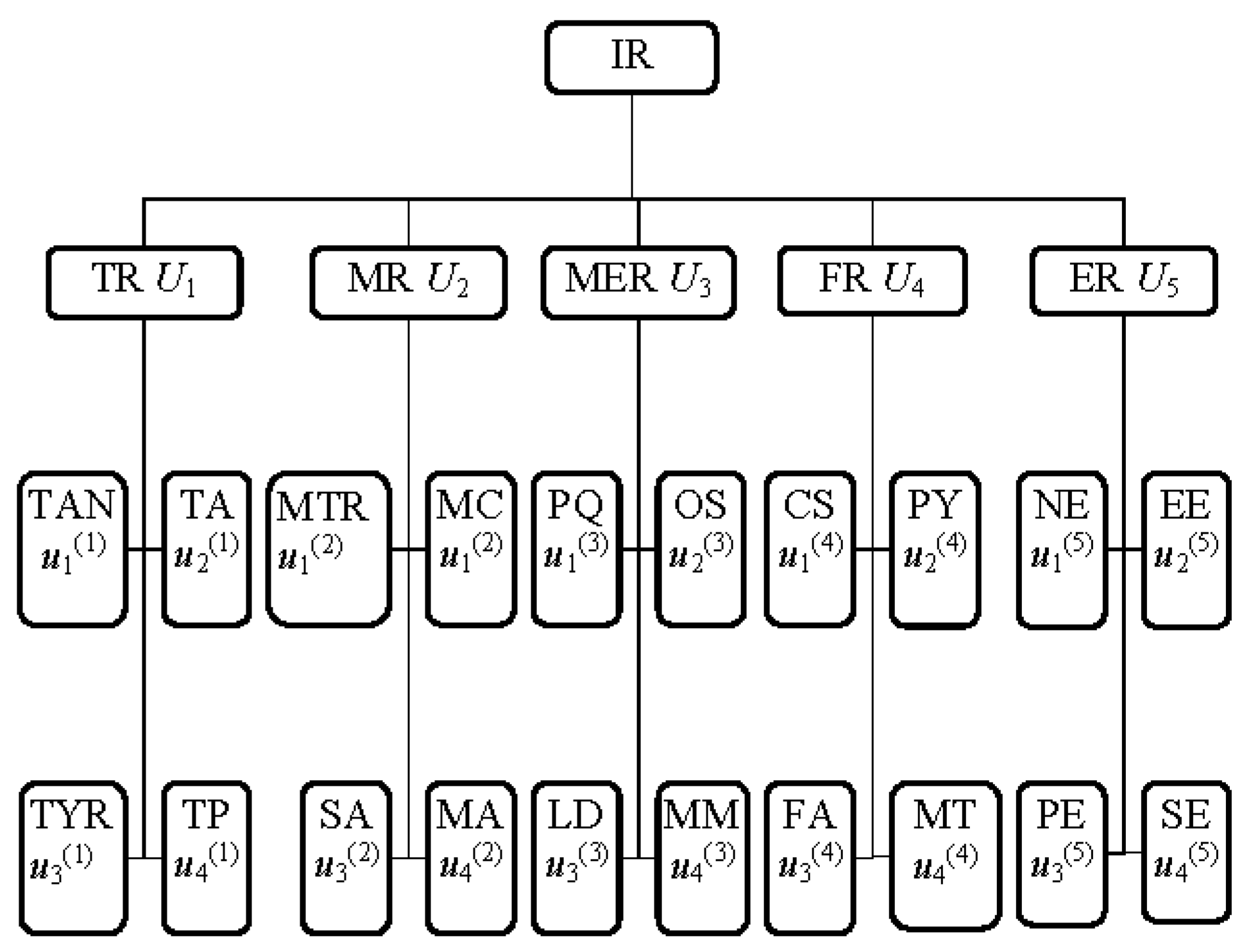
According to the principles of scientific nature, comparability and operability, we can get the investment risk multi-level evaluation index system as Figure 1 through the study of the structure and relationship analysis of venture capital investment risk factors, where IR-investment risk, TR-technical risk, MR-market risk, MER-manage risk, FR-financial risk, ER-environmental risk, TAN-technology advanced nature, TA-technology applicability, TYR-technology reliability, TP-technology periodicity, MTR-market requirement, MC-market competition, SA-sale ability, MA-market access, PQ-personnel quality, OS-organization structure, LD-leadership decision-making, MM-management mechanism, CS-capital structure, PY-profitability, FA-financing ability, MT-management ability, NE-natural environment, EE-economic environment, PE-political environment, and SE is social environment. According to the survey statistical method, we can get the factor importance degree vector W = {(0.5, 0.2, 0.1), (0.6, 0.1, 0.2), (0.4, 0.3, 0.3), (0.3, 0.1, 0.5), (0.3. 0.2, 0.3)}, W(1) = {(0.3, 0.1, 0.4), (0.4, 0.3, 0.2), (0.2, 0.3, 0.4), (0.4, 0.2, 0.2)}, W(2) = {(0.2, 0.2, 0.5), (0.5, 0.1, 0.1), (0.2, 0.3, 0.3), (0.3, 0.4, 0.1)}, W(3) = {5}, W(4) = {(0.6, 0.1, 0.2), (0.4, 0.3, 0.1), (0.2, 0.6, 0.1), (0.3, 0.5, 0.2)}, W(5) = {(0.5, 0.3, 0.1), (0.3, 0.2, 0.2), (0.4, 0.1, 0.2), (0.3, 0.4, 0.2)}, decision makers get the picture fuzzy evaluation matrix about a certain item risk investment projects through the information integration:
Then, according to step 4, we can get the second level comprehensive evaluation vector:
A(1) = W(1) ° R(1) = {((0.3, 0.1, 0.4) ∧2 (0.3, 0.2, 0.1)) ∨2 ((0.4, 0.3, 0.2) ∧2 (0.2, 0.6, 0.1)) ∨2 ((0.2, 0.3, 0.4) ∧2 (0.6, 0.1, 0.1)) ∨2 ((0.4, 0.2, 0.2) ∧2 (0.5, 0.1, 0.2)), ((0.3, 0.1, 0.4) ∧2 (0.7, 0.1, 0.1)) ∨2 ((0.4, 0.3, 0.2) ∧2 (0.5, 0.1, 0.3)) ∨2 ((0.2, 0.3, 0.4) ∧2 (0.5, 0.3, 0.1)) ∨2 ((0.4, 0.2, 0.2) ∧2 (0.5, 0.1, 0.3)), ((0.3, 0.1, 0.4) ∧2 (0.1, 0.2, 0.6)) ∨2 ((0.4, 0.3, 0.2) ∧2 (0.6, 0.1, 0.2)) ∨2 ((0.2, 0.3, 0.4) ∧2 (0.2, 0.1, 0.5)) ∨2 ((0.4, 0.2, 0.2) ∧2 (0.6, 0.2, 0.1)), ((0.3, 0.1, 0.4) ∧2 (0.4, 0.1, 0.2)) ∨2 ((0.4, 0.3, 0.2) ∧2 (0.4, 0.2, 0.3)) ∨2 ((0.2, 0.3, 0.4) ∧2 (0.6, 0.1, 0.2)) ∨2 ((0.4, 0.2, 0.2) ∧2 (0.3, 0.4, 0.2)), ((0.3, 0.1, 0.4) ∧2 (0.4, 0.1, 0.4)) ∨2 ((0.4, 0.3, 0.2) ∧2 (0.1, 0.6, 0.1)) ∨2 ((0.2, 0.3, 0.4) ∧2 (0.3, 0.2, 0.4)) ∨2 ((0.4, 0.2, 0.2) ∧2 (0.3, 0.1, 0.4))}
= {(0.4, 0.2, 0.2), (0.4, 0.3, 0.3), (0.4, 0.3, 0.2), (0.4, 0, 0.2), (0.3, 0, 0.2)}.
= {(0.4, 0.2, 0.2), (0.4, 0.3, 0.3), (0.4, 0.3, 0.2), (0.4, 0, 0.2), (0.3, 0, 0.2)}.
With the same way, we have
- A(2) = {(0.3, 0.3, 0.2), (0.5, 0.1, 0.1), (0.4, 0.3, 0.2), (0.3, 0.3, 0.2), (0.4, 0, 0.1)};
- A(3) = {(0.3, 0, 0.2), (0.3, 0.5, 0.1), (0.4, 0, 0.1), (0.4, 0, 0.2), (0.3, 0.5, 0.1)};
- A(4) = {(0.6, 0.1, 0.2), (0.3, 0.4, 0.2), (0.3, 0.3, 0.2), (0.5, 0, 0.1), (0.4, 0, 0.2)};
- A(5) = {(0.3, 0, 0.1), (0.4, 0, 0.2), (0.4, 0.2, 0.2), (0.4, 0.4, 0.2), (0.5, 0.3, 0.1)}.
Then, according to step 5, we can get the first level comprehensive evaluation vector:
B = W ° A
b1 = ((0.5, 0.2, 0.1) ∧2 (0.4, 0.2, 0.2)) ∨2 ((0.6, 0.1, 0.2) ∧2 (0.3, 0.3, 0.2)) ∨2 ((0.4, 0.3, 0.3) ∧2 (0.3, 0, 0.2)) ∨2 ((0.3, 0.1, 0.5) ∧2 (0.6, 0.1, 0.2)) ∨2 ((0.3, 0.2, 0.3) ∧2 (0.3, 0, 0.1)) = (0.4, 0.2, 0.2);
In addition, we have b2 = (0.5, 0.3, 0.2); b3 = (0.4, 0.3, 0.2); b4 = (0.4, 0, 0.2); b5 = (0.4, 0.4, 0.2).
Therefore, B = W ° A = {(0.4, 0.2, 0.2), (0.5, 0.3, 0.2), (0.4, 0.3, 0.2), (0.4, 0, 0.2), (0.4, 0.4, 0.2)}.
Next, we compare the size of each element in B by the scoring function and accurate function in Definition 7, and according to the principle of maximum membership, get the final evaluation result.
So, S(b1) = 0.4 − 0.2 = 0.2, S(b2) = 0.3, S(b3) = 0.2, S(b4) = 0.2, S(b5) = 0.2. H(b1) = 0.4 + 0.2 + 0.2 = 0.8, H(b2) = 1, H(b3) = 0.9, H(b4) = 0.6, and H(b5) = 1.
Therefore, we get b2 ⊱ b5 ⊱ b3 ⊱ b1 ⊱ b4.
Hence, the risk rating for the evaluation scheme is “larger risk”.
7. Conclusions
In this paper, we investigate some new operations of picture fuzzy relations and discussed their properties. The kernels and closures of a picture fuzzy relation are defined and their properties are obtained. Then, we proposed a new composition operation of picture fuzzy relations and found a new method to solve picture fuzzy comprehensive evaluation problems. In addition, we prove it is feasible by an application example.
Acknowledgments
This work was supported by the National Natural Science Foundation of China (Grant Nos. 61573240, 61473239) and Graduate Student Innovation Project of Shanghai Maritime University 2017ycx082.
Author Contributions
All authors have contributed equally to this paper.
Conflicts of Interest
The authors declare no conflicts of interest.
References
- Zadeh, L.A. Fuzzy sets. Inf. Control. 1965, 8, 338–353. [Google Scholar] [CrossRef]
- Zhang, X.H.; Pei, D.W.; Dai, J.H. Fuzzy Mathematics and Rough Set Theory; Tsinghua University Press: Beijing, China, 2013. [Google Scholar]
- Zhang, X.H. Fuzzy anti-grouped filters and fuzzy normal filters in pseudo-BCI algebras. J. Intell. Fuzzy Syst. 2017, 33, 1767–1774. [Google Scholar] [CrossRef]
- Atanassov, K.T. Intuitionistic fuzzy sets. Fuzzy Sets. Syst. 1986, 20, 87–96. [Google Scholar] [CrossRef]
- Jun, Y.B.; Ahn, S.S. On hesitant fuzzy filters in BE-algebras. J. Comput. Anal. Appl. 2017, 22, 346–358. [Google Scholar]
- Torra, V. Hesitant fuzzy sets. Int. J. Intell. Syst. 2010, 25, 529–539. [Google Scholar] [CrossRef]
- Wei, G.W.; Alsaadi, F.E.; Hayat, T.; Alsaedi, A. Hesitant fuzzy linguistic arithmetic aggregation operators in multiple attribute decision making. Iran. J. Fuzzy Syst. 2016, 13, 1–16. [Google Scholar]
- Xu, Z.S. Hesitant Fuzzy Sets Theory; Springer: Cham, Switzerland, 2014. [Google Scholar]
- Molodtsov, D.A. Soft set theory-first results. Comput. Math. Appl. 1999, 37, 19–31. [Google Scholar] [CrossRef]
- Qin, K.Y.; Hong, Z.Y. On soft equality. J. Comput. Appl. Math. 2010, 234, 1347–1355. [Google Scholar] [CrossRef]
- Zhan, J.M.; Liu, Q.; Herawan, T. A novel soft rough set: Soft rough hemirings and corresponding multicriteria group decision making. Appl. Soft Comput. 2017, 54, 393–402. [Google Scholar] [CrossRef]
- Akram, M.; Feng, F.; Saeid, A.B.; Leoreanu-Fotea, V. A new multiple criteria decision-making method based on bipolar fuzzy soft graphs. Iran. J. Fuzzy Syst. 2017. [Google Scholar] [CrossRef]
- Dai, J.H.; Han, H.F.; Zhang, X.H. Catoptrical rough set model on two universes using granule-based definition and its variable-precision extensions. Inf. Sci. 2017, 390, 70–81. [Google Scholar] [CrossRef]
- Pawlak, Z. Rough sets. Int. J. Inf. Comput. Sci. 1982, 11, 341–356. [Google Scholar] [CrossRef]
- Shakiba, A.; Hooshmandasl, M.R.; Davvaz, B.; Fazeli, S.A.S. S-approximation spaces: A fuzzy approach. Iran. J. Fuzzy Syst. 2017, 14, 127–154. [Google Scholar]
- Wang, C.Z.; Shao, M.W.; He, Q. Feature subset selection based on fuzzy neighborhood rough sets. Knowl.-Based Syst. 2016, 111, 173–179. [Google Scholar] [CrossRef]
- Zhang, X.H.; Zhou, B.; Li, P. A general frame for intuitionistic fuzzy rough sets. Inf. Sci. 2012, 216, 34–49. [Google Scholar] [CrossRef]
- Livi, L.; Sadeghian, A. Granular computing, computational intelligence, and the analysis of non-geometric input spaces. Granul. Comput. 2016, 1, 13–20. [Google Scholar] [CrossRef]
- Sanchez, M.A.; Castro, J.R.; Castillo, O.; Mendoza, O. Fuzzy higher type information granules from an uncertainty measurement. Granul. Comput. 2017, 2, 95–103. [Google Scholar] [CrossRef]
- Yao, Y. A triarchic theory of granular computing. Granul. Comput. 2016, 1, 145–157. [Google Scholar] [CrossRef]
- Peters, G.; Weber, R. DCC: A framework for dynamic granular clustering. Granul. Comput. 2016, 1, 1–11. [Google Scholar] [CrossRef]
- Skowron, A.; Jankowski, A.; Dutta, S. Interactive granular computing. Granul. Comput. 2016, 1, 95–113. [Google Scholar] [CrossRef]
- Dubois, D.; Prade, H. Bridging gaps between several forms of granular computing. Granul. Comput. 2016, 1, 115–126. [Google Scholar] [CrossRef]
- Ciucci, D. Orthopairs and granular computing. Granul. Comput. 2016, 1, 159–170. [Google Scholar] [CrossRef]
- Wang, G.; Li, Y.; Li, X. Approximation performance of the nonlinear hybrid fuzzy system based on variable universe. Granul. Comput. 2017, 2, 73–84. [Google Scholar] [CrossRef]
- Cai, M.; Li, Q.; Lang, G. Shadowed sets of dynamic fuzzy sets. Granul. Comput. 2017, 2, 85–94. [Google Scholar] [CrossRef]
- Huang, B.; Li, H.X. Distance-based information granularity in neighborhood-based granular space. Granul. Comput. 2017. [Google Scholar] [CrossRef]
- Cuong, B.C. Picture Fuzzy Sets-First Results, Part 1, Seminar “Neuro-Fuzzy Systems with Applications”; Preprint 03/2013 and Preprint 04/2013; Institute of Mathematics: Hanoi, Vietnam, 2013. [Google Scholar]
- Cuong, B.C. Picture fuzzy sets. J. Comput. Sci. Cybern. 2014, 30, 409–420. [Google Scholar]
- Cuong, B.C.; Hai, P.V. Some fuzzy logic operators for picture fuzzy sets. In Proceedings of the IEEE Seventh International Conference on Knowledge and Systems Engineering, Ho Chi Minh, Vietnam, 8–10 October 2015; pp. 132–137. [Google Scholar]
- Son, L.H.; Thong, P.H. Some novel hybrid forecast methods based on picture fuzzy clustering for weather nowcasting from satellite image sequences. Appl. Intell. 2017, 46, 1–15. [Google Scholar] [CrossRef]
- Son, L.H.; Viet, P.V.; Hai, P.V. Picture inference system: A new fuzzy inference system on picture fuzzy set. Appl. Intell. 2017, 46, 652–669. [Google Scholar] [CrossRef]
- Wang, C.Y.; Zhou, X.Q.; Tu, H.N.; Tao, S.D. Some geometric aggregation operators based on picture fuzzy sets and their application in multiple attribute decision making. Ital. J. Pure Appl. Math. 2017, 37, 477–492. [Google Scholar]
- Wei, G.W.; Alsaadi, F.E.; Hayat, T.; Alsaedi, A. Projection models for multiple attribute decision making with picture fuzzy information. Int. J. Mach. Learn. Cybern. 2016, 1–7. [Google Scholar] [CrossRef]
- Blin, J.M. Fuzzy Relations in Group Decision Theory. J. Cybern. 1974, 4, 17–22. [Google Scholar] [CrossRef]
- Cock, M.D.; Kerre, E.E. On (un) suitable fuzzy relations to model approximate equality. Fuzzy Sets. Syst. 2003, 133, 137–153. [Google Scholar] [CrossRef]
- Tamura, S.; Higuchi, S.; Tanaka, K. Pattern Classification Based on Fuzzy Relations. IEEE Trans. Syst. Man Cybern. 1971, 1, 61–66. [Google Scholar] [CrossRef]
- Yang, M.S.; Shih, H.M. Cluster analysis based on fuzzy relations. Fuzzy Sets. Syst. 2001, 120, 197–212. [Google Scholar] [CrossRef]
- Dai, W.Y.; Zhou, C.M.; Lei, Y.J. Information security evaluation based on multilevel intuitionistic fuzzy comprehensive method. Microelectron. Comput. 2009, 26, 75–179. [Google Scholar]
- Jin, J.L.; Wei, Y.M.; Ding, J. Fuzzy comprehensive evaluation model based on improved analytic hierarchy process. J. Hydraul. Eng. 2004, 3, 65–70. [Google Scholar]
- Qi, F.; Yang, S.W.; Feng, X. Research on the Comprehensive Evaluation of Sports Management System with Interval-Valued Intuitionistic Fuzzy Information. Bull. Sci. Technol. 2013, 2, 031. [Google Scholar]
- Burillo, P.; Bustince, H. Intuitionistic fuzzy relations (Part I). Mathw. Soft Comput. 1995, 2, 5–38. [Google Scholar]
- Bustinee, H. Construction of intuitionistic fuzzy relations with predetermined properties. Fuzzy Sets. Syst. 2000, 109, 379–403. [Google Scholar] [CrossRef]
- Lei, Y.J.; Wang, B.S.; Miao, Q.G. On the intuitionistic fuzzy relations with compositional operations. Syst. Eng. Theory Pract. 2005, 25, 30–34. [Google Scholar]
- Yang, H.L.; Li, S.G. Restudy of intuitionistic fuzzy relations. Syst. Eng. Theory Pract. 2009, 29, 114–120. [Google Scholar]
Figure 1.
Risk evaluation index system.


Table 1.
A picture fuzzy relation R.
| R | y1 | y2 |
|---|---|---|
| x1 | (0.3, 0.2, 0.1) | (0.5, 0.1, 0.3) |
| x2 | (0.2, 0.6, 0.2) | (0.2, 0.1, 0.5) |
Table 2.
The inverse R−1 of R.
| R−1 | y1 | y2 |
|---|---|---|
| x1 | (0.3, 0.2, 0.1) | (0.2, 0.6, 0.2) |
| x2 | (0.5, 0.1, 0.3) | (0.2, 0.1, 0.5) |
Table 3.
The complement Rc2 of R.
| Rc2 | y1 | y2 |
|---|---|---|
| x1 | (0.1, 0.6, 0.3) | (0.2, 0, 0.2) |
| x2 | (0.3, 0.2, 0.5) | (0.5, 0.3, 0.2) |
Table 4.
A picture fuzzy relation P.
| P | y1 | y2 |
|---|---|---|
| x1 | (0.5, 0.2, 0.3) | (0.3, 0.2, 0.4) |
| x2 | (0.6, 0.1, 0.2) | (0.7, 0.1, 0.1) |
Table 5.
A picture fuzzy relation Q.
| Q | y1 | y2 |
|---|---|---|
| x1 | (0.4, 0.1, 0.2) | (0.2, 0.1, 0.1) |
| x2 | (0.2, 0.2, 0.5) | (0.1, 0.4, 0.2) |
Table 6.
The picture fuzzy relation (R ∩2 P) ∪2 Q.
| (R ∩2 P) ∪2 Q | y1 | y2 |
|---|---|---|
| x1 | (0.4, 0.1, 0.2) | (0.3, 0, 0.1) |
| x2 | (0.2, 0.6, 0.2) | (0.2, 0, 0.2) |
Table 7.
The picture fuzzy relation (R ∩2 Q) ∪2 (P ∩2 Q).
| (R ∩2 Q) ∪2 (P ∩2 Q) | y1 | y2 |
|---|---|---|
| x1 | (0.4, 0.4, 0.2) | (0.3, 0, 0.1) |
| x2 | (0.2, 0.6, 0.2) | (0.2, 0, 0.2) |
Table 8.
The picture fuzzy relation (R ∪2 P) ∩2 Q.
| (R ∪2 P) ∩2 Q | y1 | y2 |
|---|---|---|
| x1 | (0.4, 0.1, 0.2) | (0.2, 0.5, 0.3) |
| x2 | (0.2, 0.2, 0.5) | (0.1, 0.4, 0.2) |
Table 9.
The picture fuzzy relation (R ∩2 Q) ∪2 (P ∩2 Q).
| (R ∩2 Q) ∪2 (P ∩2 Q) | y1 | y2 |
|---|---|---|
| x1 | (0.4, 0, 0.2) | (0.2, 0.5, 0.3) |
| x2 | (0.2, 0.2, 0.5) | (0.1, 0.4, 0.2) |
Table 10.
A picture fuzzy relation R.
| R | z1 | z2 | z3 |
|---|---|---|---|
| z1 | (0.3, 0.2, 0.1) | (0.5, 0.1, 0.3) | (0.3, 0.2, 0.4) |
| z2 | (0.2, 0.6, 0.2) | (0.2, 0.1, 0.5) | (0.6, 0.1, 0.2) |
| z3 | (0.7, 0.1, 0.1) | (0.4, 0.1, 0.2) | (0.2, 0.2, 0.5) |
Table 11.
The anti-reflexive kernel ar(R) of R.
| ar(R) | z1 | z2 | z3 |
|---|---|---|---|
| z1 | (0, 0, 1) | (0.5, 0.1, 0.3) | (0.3, 0.2, 0.4) |
| z2 | (0.2, 0.6, 0.2) | (0, 0, 1) | (0.6, 0.1, 0.2) |
| z3 | (0.7, 0.1, 0.1) | (0.4, 0.1, 0.2) | (0, 0, 1) |
Table 12.
The symmetric kernel s(R) of R.
| s(R) | z1 | z2 | z3 |
|---|---|---|---|
| z1 | (0.3, 0.2, 0.1) | (0.2, 0.5, 0.3) | (0.3, 0.2, 0.4) |
| z2 | (0.2, 0.5, 0.3) | (0.2, 0.1, 0.5) | (0.4, 0.1, 0.2) |
| z3 | (0.3, 0.2, 0.4) | (0.4, 0.1, 0.2) | (0.2, 0.2, 0.5) |
Table 13.
The reflexive closure (R) of R.
| (R) | z1 | z2 | z3 |
|---|---|---|---|
| z1 | (1, 0, 0) | (0.5, 0.1, 0.3) | (0.3, 0.2, 0.4) |
| z2 | (0.2, 0.6, 0.2) | (1, 0, 0) | (0.6, 0.1, 0.2) |
| z3 | (0.7, 0.1, 0.1) | (0.4, 0.1, 0.2) | (1, 0, 0) |
Table 14.
The symmetric closure (R) of R.
| (R) | z1 | z2 | z3 |
|---|---|---|---|
| z1 | (0.3, 0.2, 0.1) | (0.5, 0, 0.2) | (0.7, 0.1, 0.1) |
| z2 | (0.5, 0, 0.2) | (0.2, 0.1, 0.5) | (0.6, 0.1, 0.2) |
| z3 | (0.7, 0.1, 0.1) | (0.6, 0.1, 0.2) | (0.2, 0.2, 0.5) |
© 2017 by the authors. Licensee MDPI, Basel, Switzerland. This article is an open access article distributed under the terms and conditions of the Creative Commons Attribution (CC BY) license (http://creativecommons.org/licenses/by/4.0/).
Share and Cite
MDPI and ACS Style
Bo, C.; Zhang, X. New Operations of Picture Fuzzy Relations and Fuzzy Comprehensive Evaluation. Symmetry 2017, 9, 268. https://doi.org/10.3390/sym9110268
AMA Style
Bo C, Zhang X. New Operations of Picture Fuzzy Relations and Fuzzy Comprehensive Evaluation. Symmetry. 2017; 9(11):268. https://doi.org/10.3390/sym9110268
Chicago/Turabian StyleBo, Chunxin, and Xiaohong Zhang. 2017. "New Operations of Picture Fuzzy Relations and Fuzzy Comprehensive Evaluation" Symmetry 9, no. 11: 268. https://doi.org/10.3390/sym9110268
Note that from the first issue of 2016, this journal uses article numbers instead of page numbers. See further details here.