Fast and Efficient Data Forwarding Scheme for Tracking Mobile Targets in Sensor Networks


1
School of Information Science and Engineering, Central South University, Changsha 410083, China
2
School of Software, Central South University, Changsha 410075, China
3
Department of Computer Science, Stony Brook University, Stony Brook, NY 11794, USA
4
Department of Computer Science and Technology, Huaqiao University, Quanzhou 362000 China
5
School of Information Technology in Education, South China Normal University, Guangzhou 510631, China
*
Author to whom correspondence should be addressed.
Symmetry 2017, 9(11), 269; https://doi.org/10.3390/sym9110269
Submission received: 23 October 2017
/
Revised: 5 November 2017
/
Accepted: 6 November 2017
/
Published: 9 November 2017
(This article belongs to the Special Issue Advances in Future Internet and Industrial Internet of Things)
Abstract
:Transferring emergent target tracking data to sinks is a major challenge in the Industrial Internet of Things (IIoT), because inefficient data transmission can cause significant personnel and property loss. For tracking a constantly moving mobile target, sensing data should be delivered to sinks continuously and quickly. Although there is some related research, the end to end tracking delay is still unsatisfying. In this paper, we propose a Fast and Efficient Data Forwarding (FEDF) scheme for tracking mobile targets in sensor networks to reduce tracking delay and maintain a long lifetime. Innovations of the FEDF scheme that differ from traditional scheme are as follows: firstly, we propose a scheme to transmit sensing data through a Quickly Reacted Routing (QRR) path which can reduce delay efficiently. Duty cycles of most nodes on a QRR path are set to 1, so that sleep delay of most nodes turn 0. In this way, end to end delay can be reduced significantly. Secondly, we propose a perfect method to build QRR path and optimize it, which can make QRR path work more efficiently. Target sensing data routing scheme in this paper belongs to a kind of trail-based routing scheme, so as the target moves, the routing path becomes increasingly long, reducing the working efficiency. We propose a QRR path optimization algorithm, in which the ratio of the routing path length to the optimal path is maintained at a smaller constant in the worst case. Thirdly, it has a long lifetime. In FEDF scheme duty cycles of nodes near sink in a QRR path are the same as that in traditional scheme, but duty cycles of nodes in an energy-rich area are 1. Therefore, not only is the rest energy of network fully made use of, but also the network lifetime stays relatively long. Finally, comprehensive performance analysis shows that the FEDF scheme can realize an optimal end to end delay and energy utilization at the same time, reduce end to end delay by 87.4%, improve network energy utilization by 2.65%, and ensure that network lifetime is not less than previous research.
1. Introduction
Industrial Internet of Things (IIoT) [1,2,3,4,5] as well as cloud computing [6,7,8,9,10] leverage the ubiquity of sensor-equipped devices such as smart portable devices, and smart sensor nodes to collect information at a low cost, providing a new paradigm for solving the complex sensing applications from the significant demands of critical infrastructure such as surveillance systems [11,12,13,14,15], remote patient care systems in healthcare [4,16,17], intelligent traffic management [18,19,20], automated vehicles in transportation environmental [19,20] and weather monitoring systems [21,22]. One of the important applications in this area is target tracking, which has a variety of applications such as tracking enemies, humans, animals and cars on highways, and many other cases [23,24]. In tracking applications, when nodes sense the target, they report the state information to a sink through multi-hop routing [23,24]. When the target moves to the next location, the closest node to the target continues to monitor the target, and the target continues to be monitored through the collaboration of such multiple nodes. In such mobile target monitoring applications, there are several key issues that are worth studying. (1) Delay. The delay can be divided into two categories: one is called sensing delay, referring to the time difference between nodes sensing the target or event and the target appears or the event occurs [25]. The other category is called end to end delay (or communication delay) [25]. It refers to the time that sensor nodes will be routed to sink after receiving monitoring data. In applications such as emergency and dangerous mobile target monitoring, it is important to send the status information of a mobile target to the sink quickly and continuously [26,27,28]. Therefore, excessive delay in mobile target monitoring application can affect the timeliness and accuracy of the decision, which can cause very serious losses [26,27,28]. For example, in the surveillance of an enemy, it is necessary to continuously send the status information of the enemy to the sink, so the allies can make appropriate responses to the invasion of the enemy. A longer delay will cause great danger to one’s own side; (2) Another key issue is energy consumption and network lifetime. Sensor nodes are usually powered by batteries, so their energy is extremely limited. Replacement and recharging of batteries is costly and sometimes impossible [29,30,31]. Therefore, in wireless networks, one of the main challenges in target tracking is reducing the energy consumption of each node and balancing the energy consumption in all nodes at the same time to optimize the energy consumption and maximize the network lifetime [32,33,34].
Generally speaking, sensor nodes are restricted by low capacity processing capabilities, battery operated devices, limited transmission ranges as well as limited data transmission capacity and other attributes [35,36,37,38], among which limited energy is the most influential constraint. In order to reduce energy consumption, sensor nodes often take a periodic sleep/awake rotation working model to save energy [25,27]. The ratio of the length of time the node is in the working state to the length of the cycle time is called the duty cycle. Since the energy consumption of the node during work is 100 to 1000 times that of the energy consumption in the state of sleep, nodes should be in the state of sleep as possible to save energy which means duty cycles of nodes should be small as much as possible to prolong lifetime. However, when the node is in the state of sleep, it cannot monitor the target anymore [25,27]. Therefore, a small duty cycle can have a negative effect on network monitoring and increase sensing delay and communication delay. Sensing delay and communication delay also increase with longer sleep time. Because sensing data is transferred to sink through a multi-hop routing path, each hop on routing path needs to wait for its forwarding nodes to be awakened from sleep to transmit data when a sender has data to be transferred. The time spent waiting for forwarding nodes to awaken from sleep is called sleep delay. Sleep delay is much longer than the actual amount of time it takes to send the data, so sleep delay of multi-hop relays becomes the main component of communication delay.
Although there is much research about reducing delay, most of them concentrate on reducing sensing delay. For instance, in target monitoring, the method which is proposed in Ref. [23] is more about how to proactivate nodes in which the target is ready to move, so that when the target moves to this region, it can greatly reduce its sensing delay. However, it can be seen from the previous demonstration that there is sleep delay in every hop of communication delay, and each sleep delay is comparable to the monitoring delay [5,25]. Therefore, communication delay is much more than sensing delay. In addition, the system cannot make decisions until sink receives the sensing data even if the sensing delay is very small. Thus, it is important to reduce the sensing delay, but reducing communication is even more important. However, there is little research on reducing communication, which can affect the performance of the entire system.
Reducing communication delay between target and sink is a challenging issue. Previous research concentrates on building an effective path from target to sink. And the same routing method in the network is adopted after establishing the path to make the communication delay larger [24], so that the performance of the whole target monitoring is greatly affected. Therefore, in this paper, a Fast and Efficient Data Forwarding (FEDF) scheme for tracking mobile targets in sensor networks is proposed to reduce tracking delay and maintain long lifetime. Innovations in this paper are as follows:
(1) We propose a method to transmit target sensing data through a QRR path which can reduce delay efficiently. In wireless sensor networks, energy consumption is not balanced, because in the area near the sink ahead of all sensing nodes, its energy consumption is far greater than that of the far sink area. And network lifetime depends on lifetime of the first node in the network. According to related research, the network still has as much as 90% of the energy left when it dies. Therefore, in FEDF scheme, a QRR path is created from target to sink. On QRR path, the duty cycle of nodes near the sink is the same as that in traditional scheme while the duty cycle of nodes far from sink is set to 1. Since most of the area of the network has surplus energy, on a QRR path, normally only one node's duty cycle is the same as the traditional one, while the duty cycles of other nodes are 1. In this way, when data is forwarding in this QRR path, its sleep delay will be reduced to 0, which can reduce the communication delay in target monitoring greatly.
(2) This paper presents a comprehensive approach to fast routing establishment and routing optimization in order to improve the efficiency of fast routing. The target data routing scheme in the paper belongs to trail-based routing, so the routing path gets longer and longer with the movement of target, leading to lower efficiency. We proposed QRR path optimization algorithm in this paper, in which the ratio of the routing path length to the optimal path is maintained at a smaller constant in the worst case.
(3) Finally, comprehensive performance analysis shows that FEDF scheme can realize the optimization of end to end delay and energy utilization at the same time, reduce end to end delay by 87.4%, improve network energy utilization by 2.65%, and ensure that network lifetime is not less than previous research.
The rest of this paper is organized as follows: in Section 2, a literature review related to this work is introduced. Then the system model and problem statement are described in Section 3. In Section 4, we propose an efficient FEDF scheme. The performance analysis of the FEDF scheme is provided in Section 5. Finally, Section 6 presents the conclusion and future perspectives of our work.
2. Related Work
There are already quite a few studies on tracking targets. These studies mainly focus on the following aspects.
2.1. Target Detection in Stationary Sink Network
In terms of stationary target or event monitoring [5,25], as shown in the network model shown in Figure 1, in this kind of research, sensor nodes are deployed in advance in the network, the event or target can be sensed by nodes nearby when a pre-defined event or target appears in the network. The sensing data is then sent to the sink through the shortest routing path. Apparently, in such stationary sensor and sink networks, communication delay depends mainly on factors such as the distance between the location of event or targtet and sink and the method used in data transmission. In a given network, if common data transmission methods are adopted, the communication delay is usually determined, so the main concern is to reduce the sensing delay in such networks.
Factors that affect delay involve several layers, mainly on the MAC layer, network layer, and application layer. Effective MAC protocol is a way to reduce energy consumption and delay. MAC protocol adopted by sensor network can be divided into synchronous MAC protocol [39,40] and asynchronous MAC protocol [41] according to application network it is targeting. In a synchronous wireless sensor network, nodes have the same clock frequency. The nodes wake up only when they need to work, while at other times they sleep. Such protocols are mainly TDMA protocol. The TDMA protocol [42] usually minimizes power consumption while ensuring bounded delay and fairness. However, these protocols require precise synchronization, which limits the scalability of the system.
Synchronization in a large-scale network is a very difficult thing. Therefore, in wireless sensor networks, most applications adopt asynchronous mode. In this way, each node only needs to select its own work slots independently without synchronization, thus increasing its applicability. In general, however, the performance of delay in a wireless sensor network is not as good as that in a synchronous network when working asynchronously. It is because, in the asynchronous mode, the wake/sleep cycle rotation of nodes is independently determined by each node. Periodic cycle is the most important factor in determining delay, so there is more research on duty cycle than delay [43,44]. Generally speaking, increasing duty cycle of the node can reduce sleep delay so as to reduce communication delay significantly. However, increasing the duty cycle of nodes increases the energy consumption and reduces the network lifetime. Therefore, existing researches mainly focuses on how to meet the requirement of applications’ delay in the case of minimizing the duty cycle. A dynamic duty cycle method is commonly used. In the method, we often set small duty cycle to nodes to extend network lifetime. In addition, when the amount of data increases, we increase the duty cycle of nodes, which can meet the application requirements, reduce the delay and maintain a relatively high network life. The main types that belong to the research are Demand Wakeup MAC (DW-MAC) [45] and Adaptive Scheduling MAC (AS-MAC) [46]. In the network where nodes have the same duty cycle, the larger the node density is, the larger the amount of nodes perceived by target. In addition, the target cannot be detected when sensor nodes are in the state of sleep. Therefore, the larger the node density, the smaller the sensing delay is. However, on the one hand, increasing node’s duty cycle increases the energy consumption. On the other hand, increasing the density of nodes increases the deployment cost.
2.2. Tracking Mobile Target
In mobile target networks, nodes in the network are stationary after deployment, while the target is mobile. As shown in Figure 1, the elephant is a mobile target. When the target moves into the network, the sensor node is required to perceive the target in the shortest possible time. The time difference between target appearing in the network and target being perceived is represented as sensing delay. In some research, sensing delay is also represented as the distance the target moves from its access to the network to when it is perceived by the sensor node. Meanwhile, it is necessary to send the target’s sensing information to sink continually as the target keeps moving. As is shown in Figure 1, when the target is in place A, the sensor node A perceives its information to be sent to the sink, while target moves to B, and the sensor node B perceives its information and sends it to the sink.
In fact, the perception of mobile target is far more simple than as described above, which can be divided into two methods: (i) non-collaborative target monitoring; and (ii) collaborative target monitoring. In a non-cooperative target monitoring method, nodes are randomly deployed in areas that need to be monitored. Therefore, one of the main research contents of non-cooperative target monitoring is target coverage. The purpose is to achieve thata situation in which, the target enters the monitoring area, at least one node can monitor the target. Huang et al. [17] studied the optimal placement of sensors with the goal of minimizing the number of installed devices, while ensuring coverage of target points; and wireless connectivity among sensors.
Collaborative target monitoring is achieved to monitor the target through collaboration between nodes. Such monitoring is mainly applied to monitoring mobile targets [5,6,23,24,25]. In such studies, when the mobile target is monitored by a node, the node will notify nodes of the next region that the target may move to. So continuous monitoring of the target is realized through collaboration between nodes. Obviously, this kind of monitoring method only sets the duty cycle of nodes to 1 at the possible location of the target, and the duty cycle of node in other areas is very small. Consequently, it can save energy and maintain high monitoring quality.
2.3. Target Detection in Mobile Sink Network
In such a network, sensor nodes are stationary after deployment, while the sink is mobile. The sensing delay in this kind of network is the same as the second network mentioned earlier. However, the communication delay is quite different from the previous network. In the previous network, sensor nodes and sinks are stationary, so we can know the path data routing to sink after sensor nodes sense data. However, in the mobile sink network, even if a routing path to the sink is established in the previous period, a sink may move to another location within the next period. Therefore, how the data monitored by a sensor node can be effectively routed to a mobile sink is more complicated in this kind of network, and the communication delay is larger. In such networks, because communication delay is the largest component of delay, such networks mainly focus on how to reduce communication delay. This type of network is usually applied to a mobile user, which require attractive events or targets to be sent to these mobile users (sinks).
2.4. Track Mobile Target with Mobile Sink Network
Multiple mobile targets and multiple sinks. There are also various applications of this type of network in practice [39]. As Figure 2 shows, in safari parks, visitors are equivalent to a mobile sink (user in Figure 2), and the object that attract tourists like the elephant is mobile target. Tourists is walking all the time. When sensor percieves the elephant, it informs tourists (namely mobile target) and tells them the location of elephant. Such studies generally adopt trail-based routing to maintain the route between target and sink so that the sink and target can keep up correspondence with each other. In target tracking like this, the routing trail between target and mobile sink and sink’s trail are stored in the routing path. As a result, nodes can always route to sink through these trails after sensing the target. And regardless of how target and sink moves, through trail routing, a routing path from source node to sink can always be established successfully. As is shown in Figure 2, when the target moves from A to B, user (namely mobile sink) moves from C to D. The method of establishing routing is, when mobile target (elephant) is moving, it keeps track of how it gets to A. In this way, when mobile target moves to B, the sensor node will still be able to send its sensing information to A through trail. Because routing between A and B has been established already, and when the user moves from C to D, user also retains trail between C to D. Thus, sensing data that reaches C can continue to route to user in position D. In this method, the routing from target to sink is routed through the original location, so its routing path is not optimized. As Figure 2 shows, the best routing is a straight line for routing from B to D. However, due to the mobility of target and sink, the actual routing path established is B→A→C→D whose length is twice as long as the straight line from B to D. Obviously, due to the erratic motion of target and sink, the routing path from source to sink will be longer and longer after a longer period of time, resulting in poor routing efficiency. The path to sink may actually be k hops, but the current path of source to sink could be n times as much as k. The commonly used method is, after every period of time, when the routing efficiency becomes very poor, we reestablish the straight line route from target to sink, reduce invalid path, and make its path length close to k. This method of path optimazation is also discussed in literature [24], In their method, when a detour appear on the routing path from target to sink, there will be a certain way to find the path shortcut, reduce the path length, and improve the routing efficiency.
According to the target’s attributes, the network can be divided into discrete target or event perception network and continuous target monitoring network. In discrete target or event perception network, event occurs randomly in the network. In this type of network, sensor nodes typically transmit the data perceived to sink while in continuous target monitoring network, mobile target keeps moving in the network, so sensor nodes need to transmit data to sink continuously after sensing the target.
Although there is plenty of research on tracking mobile targets, these studies mainly concentrate on how to establish a routing path from mobile target to sink. And in terms of reducing delay, they specialize in reducing sensing delay and neglect communication delay and the proposed solution is very few [47]. Furthermore, the professional methods about reducing the communication delay do not take into account the actual application of mobile target. For instance, Naveen and Kumar proposed Tunable Locally-Optimal Geographical Forwarding (T-LOGF) policy, Ref. [48] in order to reduce the communication delay. Their ideas are based on the following analysis: in the network of duty cycle working mode, each node may have multiple forwarding node sets when forwarding data, these forwarding nodes use the periodic awake/sleep mode independently. So, when the sender has data to be transferred, the first node that wakes up is not necessarily close to sink. At that time, the sender can continue to wait for a node closer to sink to wake up, or send it immediately. The disadvantages of immediate dilivery are: every time the routing distance to sink is short, more hops are needed to be routed to sink, which can cause large delay. And waiting for nodes closer to sink to wake up can make the number of hops from sink smaller. It is possible to reduce the total delay but increase the waiting delay. T-LOGF proposed an algorithm of optimizing forwarding nodes choice to reduce delay [48].
This method that only consider about routing can adopted by target tracking method. However, these routes still don’t take into account factors in tracking target, such as how to maintain the uniqueness of routing trail, and also lack of ways to optimize the routing on the basis of maintaining the characteristics of the trail. Although some studies have suggested that the adoption of improved duty cycle methods can effectively reduce delay, but improving the duty cycles of the entire network will have a significant impact on network lifetime. And as a matter of fact, target occurs locally and sporadically. If we just increase the duty cycle of nodes in these areas and on routing path, it can significantly reduce the delay and has little impact on the network lifetime. The scheme demonstrated in this paper exactly are based on this idea. The FEDF scheme proposed in this paper maintains high network lifetime on the basis of reducing delay.
3. System Model and Problem Statement
3.1. System Model
The network model in this paper belongs to a typical planar periodic data gathering wireless sensor network, which is similar to [13,23,24], and its model structure is as follows:
(1) N homogeneous sensor nodes are randomly deployed in a two-dimensional planar network whose center is sink. The network radius is R, and the node density is ρ. Each node in the network monitors the surrounding environment continuously, and once the event or target is detected, the next hop is searched in the range of the communication radius r, and the sensing data should be sent to sink through multi-hop relays.
(2) Sensor nodes adopts asynchronous sleep/wake working mode in this paper, and nodes monitor the target and transmit the data only when they are in the waking state.
(3) All the monitoring targets are randomly distributed in the network, so the probability that each node monitors target, which leads to the probability that each node generates data is equal.
3.2. Network Parameters
The component of a sensor node includes a sensing unit and a communication unit [16,19,41], in which the sensing unit is in charge of sensing the monitoring target or event and mobilizing the communication unit after sensing the target or event, then the communication unit initiates its internal communication mechanism to transmit data to sink. The sensor nodes adopt sleep/wake periodic mode to save energy for lacking of energy [17]. In a unit cycle, the nodes sleep/wake work periodically. The node only transmits data and senses targets or events when it is in the waking state. In a unit cycle, the ratio of the node in the waking state to the whole cycle called duty cycle, assume that is the sensing duty cycle and is the communication duty cycle, then:
where is the time that the node is in the waking state during the sensing cycle and is the time that the node is in the sleeping state during the sensing cycle; is the sensing duration of the node and is the communication duration of the node; is the time that the node is in the waking state during the communication cycle, and is the time that the node is in the sleeping state during the communication cycle.
The energy consumption model of this paper is similar to [14,15], and the energy consumption of nodes is mainly composed of event sensing, data transmission, data receiving and low power listening. Therefore, the energy consumption model can be expressed as:
The main parameters of the system model used in this paper are similar to [7], and the parameters values are derived from the internal data tables of the prototype sensor nodes. Table 1 and Table 2 list the relevant parameters used in this paper, the remaining parameters not in tables will be described in the specific calculation.
3.3. Problem Statement
Designing an efficient communication scheme that is suitable for wireless sensor networks is a major goal of this paper. With regard to network performance, the scheme should be able to optimize the overall performance of the network, reduce the communication delay, improve the energy utilization and maintain the network lifetime. It can be expressed as follows:
(1) Minimize communication delay
In this paper, the communication delay refers to the time it takes for data to be transferred from the sending node to the sink via multi-hop relays [19].
where stands for the transmission delay of i-th hop, and the number of relay hop is , then the minimized communication delay can be expressed as Formula (4).
(2) Maximize energy utilization
Energy utilization refers to the ratio of the energy consumed by the network to the initial energy of the network.
where stands for the initial energy of the node and the energy consumption of node is so the maximized energy utilization can be expressed as Formula (6).
(3) Maximize network lifetime
Network lifetime is defined as the death time of the first node in the network in most studies [12,20]. In wireless sensor networks, if the energy of the node is exhausted, the node will die. As a result, the network lifetime is closely related to the maximum energy consumption of the network. Assume that there are N nodes in the network, the energy consumption of node is , its initial energy is . Therefore, maximizing the network lifetime is equivalent to maximizing the lifetime of the node with the largest energy consumption, that is:
In a nutshell, the research objectives of this paper are as follows:
4. The Design of FEDF Scheme
4.1. Introduction of QRR Path
In a wireless sensor network, the sensor node has the function of sending and receiving data. In addition, in the process, there is a lot of energy consumption. Therefore, sensor nodes often take the periodic sleep/awake rotation working model in order to reduce energy consumption. Data can be sent and received only when the node is in the waking state. Therefore, when a node needs to send data to the sink, it has relatively large delay by using the traditional method, because it has to wait for the next node to wake up. In this case, the delay will be increasingly large as the routing path gets longer. We propose a method in this paper that is to create a Quickly Reacted Routing (QRR) path. On the path, the duty cycles of nodes far away from sink are set to 1, which means they are in the work state all the time. In this way, the efficiency of data transmission has been greatly improved.
Considering that most nodes on a QRR path are working all the time, the energy consumption is pretty huge. In addition, there is a phenomenon in the field of wireless sensor network called an energy hole. The energy consumption of nodes close to the sink is greater; nodes near the sink are dead in the end so as to form energy hole. The duty cycle of the nodes near the sink is set as normal. As a result, the network maintains relatively high network lifetime.
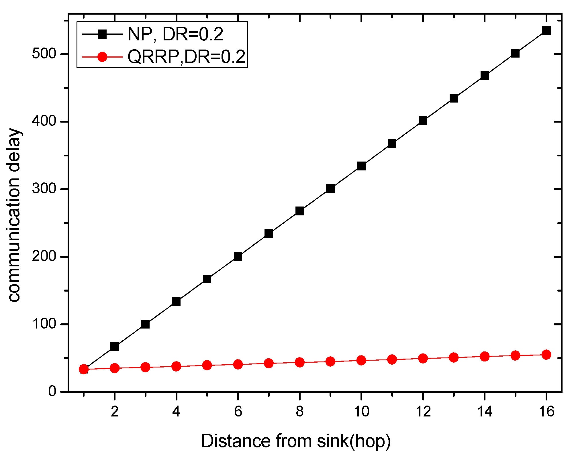
Figure 3 shows the communication delay of the network by using normal path and a QRR path. The duty cycle is 0.2. The delay of the node 1 hop away from the sink is equal. As the distance from the sink is farther and farther, the communication delay is increasing whether on the normal path or the QRR path. However, it is obvious that the communication delay on normal path is far greater than on the QRR path.
Figure 4 shows the communication delay on the normal path and QRR path under different duty cycles. NR in Figure 4 is short for normal path. Path under the same duty cycle have the same communication delay in the range of one hop from the sink. In addition, as the duty cycle is larger, the communication delay is smaller. Furthermore, the communication delay of QRR path is significantly smaller than that of normal path. It can be seen that using a QRR path to transmit data can greatly reduce the delay and improve the working efficiency of the network.
4.2. General Design of FEDF Scheme
In a wireless sensor network, the target keeps moving, and when the node senses the target, it will send the data to sink. As is shown in Figure 5, each time the node perceives the target, it goes straight through the shortest path and sends the data to the sink. However, the FEDF scheme is proposed in this paper, which can transmit data efficiently and save resources.
Before introducing the scheme, we suppose that: Firstly, according to Global Positioning System (GPS) or position assessment devices, each node knows its own coordinates. Secondly, the target moves randomly. Thirdly, each time a node is passed, the node records two messages: number of hops from sink (hopCount) and a set of nodes that have been visited (visited_list).
The scheme consists of three steps. The first step is initializing the sensor network: In a circular area of radius R, set and locate the coordinates of each node and the distance between nodes and initialize the shortest distance from them to the sink. The second step is creating an initial QRR path when the sensor node senses the target in the beginning. The third step is creating a QRR path according to the random movement of mobile target. The last step is optimization of the path.
(1) Initialize the network: determine the minimum hopCount between node and sink
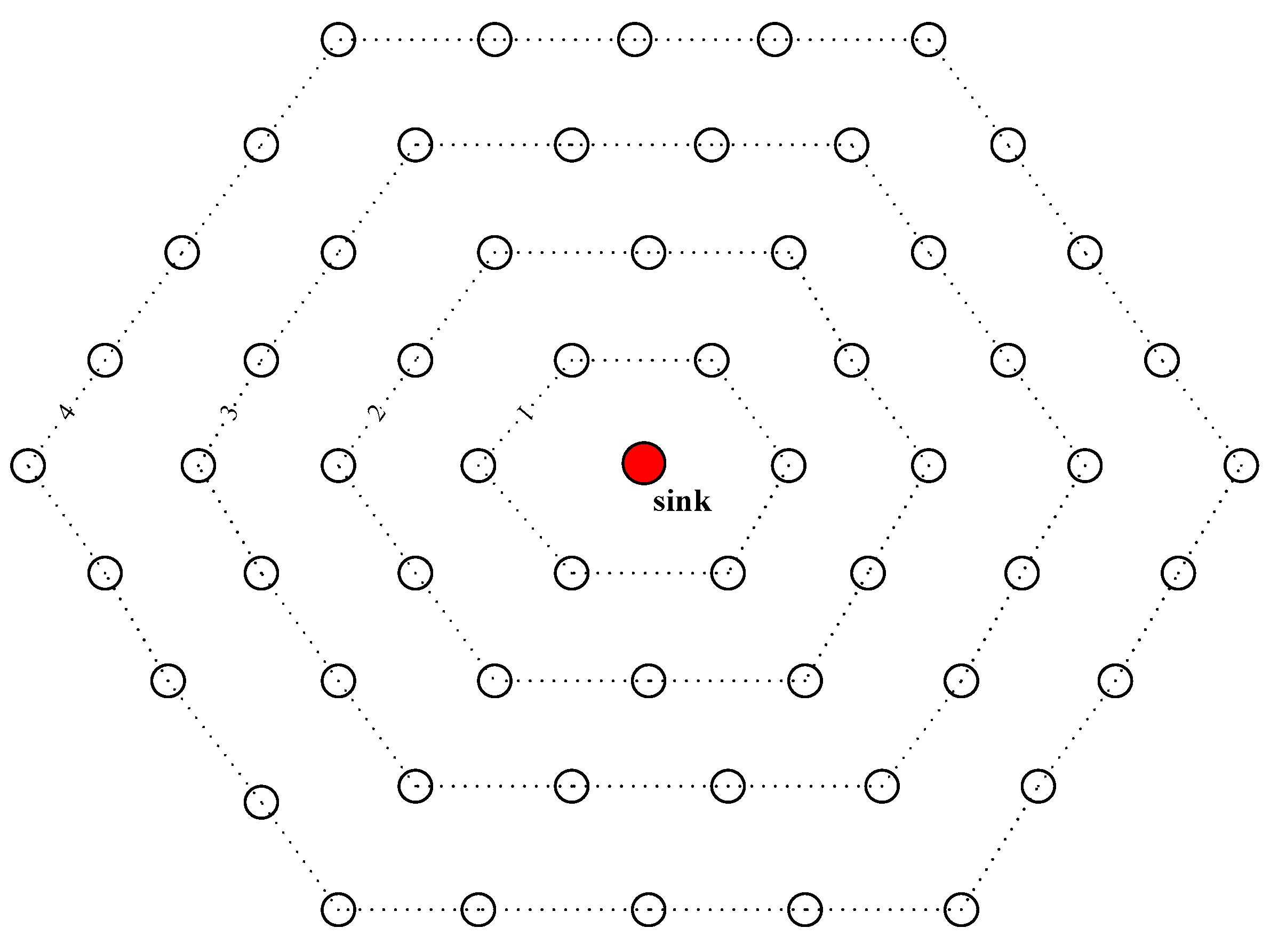
In the initial situation, there are many sensor nodes in the provided monitoring area. In this paper, we will assume that nodes in the network are uniformly distributed, which means the distances between nodes are equal. Each node knows its position in the coordinate system. In the process of initialization, we set the number of hops from sink to sink itself () to 0, while set other nodes to the sink to ∞. Then the sink broadcast is 0. When other adjacent nodes received the value, they add one to this value and continue to broadcast it. When the value of hopCount is smaller than that of itself, update the value to the smaller one and add one. Update the value of each node’s hopCount according to this method until hopCount of every node in the network is no longer changed. The network initialization is completed. Figure 6 shows the network after initializing. How to initialize the network is shown in Algorithm 1.
| Algorithm 1 Initialize the network |
| 1: Initialize = 0 2: Initialize every node in the network: = ∞ 3: sink broadcast its , and assume node’s received from others is 4: For every node in the network Do 5: If > + 1 Then 6: = + 1 7: End if 8: Else 9: keep its original value 10: End else 11: End for |
(2) Create an initial QRR path
When the sensor node senses the target, it must check its recording table (including the last node and the next node) and ensure whether there has been a QRR path. If any, the node just transmits data through it. If no, we create a QRR path according to Algorithm 2, and set duty cycles of nodes far from the sink to 1. In this way, an initial QRR path is created, as is shown in Figure 7.
The next node of is represented as , the current node is , and represents the number of hops of the node from sink.
| Algorithm 2 create a quickly reacted routing path |
| 1: While > 0 Do 2: = false 3: For each node in the network Do 4: If ( < ) Then 5: = true 6: = 7: = 8: End if 9: End For 10: End while |
(3) Tracking target
In the sensor network, a mobile target will move randomly. If we do not record its motion trail, the data will be transmitted a totally new way every time the target moves, which cannot take advantage of the QRR path that was already established. Therefore, we applied the recording table. The recording table will be updated with the movement of the target to record its trail. In addition, as every movement of the target is the hopCount from the sink plus 1, add the node visited to visited_list, and set the duty cycle of the node to 1.
Algorithm 3 updates the recording table, the Current Node is represented as CN, and the Last Node is LN.
| Algorithm 3 updating path recording table(RRT) |
| 1:begin 2: For(LN.next) LN.next = CN LN = CN 5: ++ 6: CN.DR = 1 7: add CN to visited_list 8: End for 9: End |
(4) Taking Shortcuts
Because the location of the target is constantly changing, the transmission path will be complicated and tortuous when the target moves fast. In this case, both the delay and the energy consumption are very costly. So we need to simplify the path (shortcut) when necessary, which can reduce the delay and energy consumption effectively.
With regard to the nodes in the wireless sensor network, the energy consumption is mainly composed of event sensing, data transmission, data receiving and low-power listening. So the total energy consumption of a node is as follows:
In Formula (8), stands for total energy consumption, stands for the energy consumption when the node in sensing, stand for that in sending data, stands for that in receiving data, and stand for that in sleeping. And stands for the node’s data amount for sending and receiving data. and are sending duration and communication duration respectively.
Energy consumption in sensing is as follows:
where is power consumption in sensing, is power consumption in sleeping and is sensing duty cycle.
Energy consumption in sending data is as follows:
where stands for the data packet duration, is the preamble duration and is acknowledge window duration.
Energy consumption in receiving data is as follows:
where stands for the data packet duration, is the preamble duration and is acknowledge window duration.
Energy consumption in receiving data is as follows:
where the first item in the formula represents energy consumption in receiving data, and the second represents that in sleeping.
in the formula can be expressed as follows:
In sensor network, the closer the distance to sink is, the greater the energy consumption is. Supposing that the radius of the network is R, the communication radius of the node is r, and the probability of generating data is beta , so the data amount of the node that is i meters away from sink can be represented as follows:
where + < R
Data amount of the node when sending data is equal to data amount when recieving data plus data amount produced by the node itself:
Supposing that communication duty cycle in the network is , communication duration is , so one hop transmission delay of a node is as follows:
Theorem 1.
In the network, supposing that number of hops from node N to sink is , the communication delay of the node is as follows:
Proof.
According to Formula (17), we have already known one hop transmission delay is , that is , and number of hops from sink is , is communication delay. The product of the two is communication delay from node N to sink.
In the plane, distance between a and b can be expressed as . So the distance between two points can be expressed as follows:
☐
Theorem 2.
In a wireless network with uniformly distributed nodes, distance between two adjacent nodes is d, so the communication delay from node to node is as follows:
Proof.
According to Formula (19), the distance between and is , and distance between two adjacent nodes is d, so /d represents number of hops from node to , the communication delay between two nodes is the product of the hopCount from sink and one hop delay. ☐
Theorem 3.
In FEDF scheme, one hop delay of a hotpot is expressed as follows:
Proof.
According to Formula (17), in FEDF scheme, communication duty cycle of the node is set to 1, so the value of is 0. One hop delay of the hotspot is only related to , , . ☐
Theorem 4.
In FEDF scheme, number of hops from node to is , the end to end delay between two nodes with high communication duty cycle is expressed as follows:
Proof.
As for nodes separated by hops, the communication delay is the product of one hop delay and hopCount. And one hop delay of a hotpot is according to Formula (21), so the result is (). ☐
Theorem 5.
In FEDF scheme, total cost in the process of node sending data to can be expressed as follows:
Proof.
Communication delay between two nodes with high duty cycle is according to Formula (22), and energy consumption of node according to Formula (8), so the total cost of a node with high communication duty cycle is the sum of cost on delay and on energy consumption, that is + .
Theorem 6.
Similarly, the transmission cost from node to node with nomal communication duty cycle is as follows:
Proof.
According to Formula (20), the communication delay between nodes with normal communication duty cycle is (/d)(), and energy consumption of the node is according to Formula (8). So when node send data through i nodes to node , the total energy consumption is . Compared to QRR path, it has less energy consumption.
Theorem 7.
In FEDF Scheme, in order to measure the cost of sending data, we set influence factor , indicates the influence level of taking the original path and creating new path in the process of data transmission. Total cost of transmission of a node is expressed as follows:
Proof.
For a node that needs to send data, its cost in the entire process of transferring data is the sum of the cost through existing path and create a new path. According to Formula (23), the cost for the node transferring data through the existing path is () + , and the cost for the node creating a new path is (/d)() + . In addition, and stands for the degree to which these two items matter. Therefore, the total cost is expressed as Formula (25). ☐
(1) Pre-Shortcuts
We do not know which situation is the best before actually take shortcuts. Therefore, exploring a relatively appropriate path is necessary. We synthesize a variety of situations and finally choose the best as the final transmission path. The process is called pre-shortcuts in this paper.
The endpoint of a shortcut is called EDP. Every time the sensor node perceives the target, the cost of every node in its visited_list will be calculated and analyzed through Algorithm 4, including the delay and energy consumption. Thus, the node that has the minimum cost is the EDP. The implementation of the procedure will be analyzed in detail.
When the target moves to the position of node source, distance between every node p (including sink) in visited_list and source is calculated and the result is . And it is known to all that distance between two adjacent nodes is d, so /d stands for the minimum hopCount from node p to source (). In the condition that reaches a threshold η, the cost of creating a path from source to p can be calculated according to Formula (24), and the cost of transmitting data from source to sink can also be caculated according to Formula (23). Therefore, the total cost is + according to Formula (25). However, it is unnecessary to create a new path if transmitting data through the original path, and its cost is = .
In Algorithm 4, it shows the method about how to find possible EDP (pEDP).
| Algorithm 4 Identifying the possible EDPs |
| 1: Find_pEDP (Node source, Threshold η) 2: Begin 3: //η: threshold for shortcuts 4: //pre_list: the set of pEDP 5: For each node p in source.Visited _list Do 6: If (η) Then 7: Calculate of p 8: add p to pre_list 9: End if 10: End for 11: End |
In Algorithm 5, for every node in pre_list, the node that has the minimum will be found and it is exactly EDP.
| Algorithm 5 Determining the EDP |
| 1: begin 2: For each node in pre_list 3: Find min{ + } 4: return p 5: End for 6: End |
In order to reduce unnecessary delay and energy consumption, we take the shortest path when creating path, as is shown in Algorithm 6. Supposing the location of node is (), the location of source is (x, y). According to Formula (26), the offset of the abscissa and the ordinate of A (the next hop of source) can be calculated as (x.offset, y.offset) = (a, b). So nextHop(x, y) = (x-x.offset, y-y.offset).
In Formula (26), k is the slope of the straight line formed by sink and source, the location of sink is (), the location of source is (x, y), a, b stands for the offset of the abscissa and the ordinate of source respectively, and d stands for the shortest distance from source to .
| Algorithm 6 Creating a straight line path |
| 1: Find_Nexthop (NH) 2: begin 3: //NH: next hop 4: If (NH is not sink) Then 5: nextHop(x, y) = (x-x.offset, y-y.offset) 6: If (search_neighbor (nextHop) != NULL) Then 7: return nextHop 8: End if 9: End if 10: End |
(2) Taking Shortcuts
After the final EDP is determined, the target sends a data packets from the source to the EDP to inform it of the two ends of the shortcut. According to Algorithm 6, the next hop is found continuously and every time a node is visited, its recording table is updated, and its communication duty cycle is set to 1. Until the next hop is the EDP, the original path can be cancelled, which means restoring the duty cycle of nodes on the path and deleting relevant items of the recording table. Before that, data is transmitted through the original path.
As is shown in Figure 8, the target sends data from source to sink through A-B-C-D-E-F-G. Assuming that the value of η is 2, the cost of nodes (except for node A an B) in visited_list can be calculated according to Algorithm 6, and add pEDPs to pre_list.
We compare the cost of all nodes in pre_list according to Algorithm 5, assuming that the node that has the minimum cost is F, F is EDP in the example. Therefore, the target send a information packet from source to F to inform F, according to Algorithm 6, the sending path is H→I→F. Before the arrival of data packet, target transmit data through the original path. When the packet arrives, cancel path A→B→C→D→E→F, restore their duty cycle, remove them from visited_list and delete the relevant information of recording table. Since then, the target will send data data through path H→I→F→G.
5. Performance Analysis of FEDF Scheme
In this paper, we measure the performance of a FEDF scheme from three aspects: delay, energy utilization and network life. By analyzing and comparing the performance of the FEDF scheme and the traditional routing scheme (every time take the shortest way), compared to traditional scheme, the FEDF scheme reduces communication delay by 87.4%, and improves energy utilization by 2.65%. It is obvious that the FEDF scheme demonstrated in this paper performs extremely efficiently.
In the sensor network, the distance between two adjacent nodes is d. A mobile target keeps moving and moves randomly in all directions in the network, which produces a variety of paths. So in the mathematical statistics point of view, the probability that each node moves in every direction is equal. That is, the actual path (D) of the mobile target and its distance (d) to the sink are proportional. Therefore, we can set a path simplification coefficient λ (λ ≥ 1) and D = d × λ. For different scenarios, the value of λ is different. For instance, when the mobile target moves fast and the path bending degree is large, the value of λ is larger. However, when the velocity is slow, the path is similar to a straight line, and the value of λ is small and close to 1. We will analyze the delay and energy consumption in the case of different values of λ below.
5.1. Transmission Delay
Theorem 8.
In FEDF scheme, assume that the network radius is R, the communication radius is r, the set of nodes with communication duty cycle of 1 is , the set of nodes with common duty cycle is , and one hop delay of node n can be expressed as follows:
Proof.
according to Formula (17), one hop delay of node with normal communication duty cycle is , and according to Formula (21), one hop delay of node with duty cycle of 1 is . In summary, one hop delay of a node can be expressed as Formula (27). ☐
Theorem 9.
In FEDF scheme, on QRR path, the duty cycle of node near sink is normal, others is 1. HopCount from node n to is , and these nodes has high duty cycle. Therefore, the communication delay from node n to sink can be expressed as follows:
Proof.
One hop delay of nodes with normal duty cycle is from Theorem 8, so one hop delay of is . And the duty cycle of other nodes is 1, the sum of the delay of these nodes is (). Therefore, the communication delay from node n to sink is as Formula (28). ☐
In the FEDF scheme, on a QRR path, the first hop from the sink has a normal duty cycle, while other nodes have a duty cycle of 1. However, in the traditional routing path (TRP) scheme, the communication delay is directly proportional to distance from the sink.
Figure 9 shows the communication delay comparison of the FEDF scheme and the TRP scheme, in which the routing path is straight; the value of λ is 1.
When the degree of bending of the path is different, the communication delay is different. In general, the longer the path, the larger the delay. Figure 10 shows the performance of the communication delay in the FEDF scheme from different λ as the distance from the sink becomes larger. It is obvious that the communication delay is large if the value of λ is large.
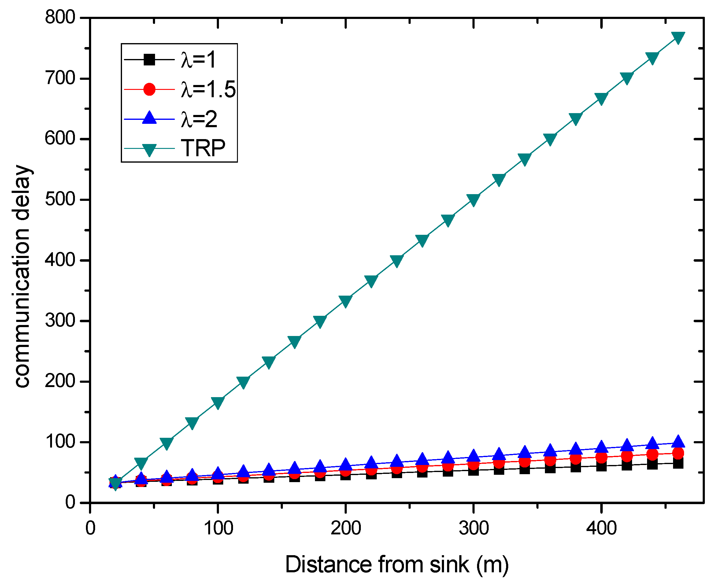
Figure 11 shows the communication delay in FEDF from different λ and in TRP. When λ is 2, the communication delay in the FEDF scheme is greatly less than that of the TRP scheme. In general, the value of λ will be maintained at a relatively small number, because every time the value of λ becomes relatively large, that is, when the degree of the path bending gets large, the path will be updated according the algorithm. In a word, with regard to delay, the FEDF scheme performs very well.
5.2. Energy Utilization
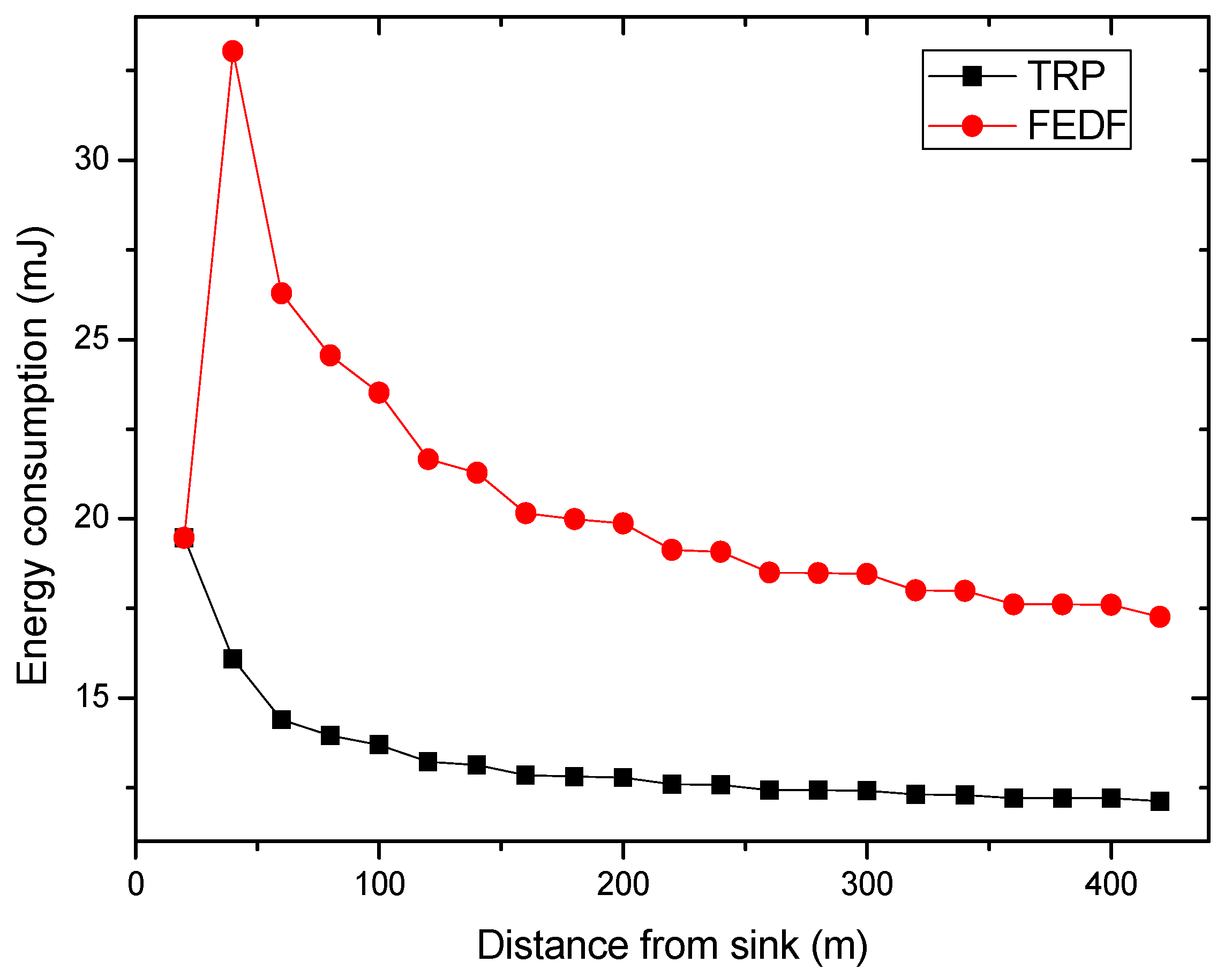
Figure 12 shows the energy consumption of the TRP scheme and the FEDF scheme in the case of the communication duty cycle being 0.2. In general, the closer the sink, the greater the amount of data the node needs to forward, and the severer the energy consumption. The closer the node is to the sink, the greater the data amount that the node needs to forward, and the more the energy consumption will be. However, the first hop from the sink has normal duty cycle in the FEDF scheme, so several nodes far away from sink have more energy consumption. Energy consumption is larger in the FEDF scheme than in the TRP scheme, but the former can improve the energy utilization of the network.
What should be emphasized is that, in Figure 12, we only consider nodes on just one path. As a matter of fact, nodes that one hop away from sink have larger energy consumption than that two hops away from sink. Therefore, the curve should show a downward trend. Assume that the network communication radius is r and the node density is . There are nodes that one hop away from sink, there are nodes that two hops away from sink, there are nodes that three hops away from sink. In addition, the average energy consumption of nodes that have the same distance from sink is the sum of their energy consumption divided by the number of nodes. As a result, node’s energy consumption reduces as its distance from sink increases.
Theorem 10.
In the wireless sensor network, there are n nodes, the average energy consumption of each node is , so energy consumption of the network can be expressed as follows:
Proof.
The network energy utilization is the ratio of the total energy consumed by the entire network to the total maximal energy that can be consumed. Total energy consumption can be calculated according to Formula (8).
Figure 13 shows the energy utilization in TRP scheme and FEDF scheme. Compared to TRP scheme, FEDF scheme can improve the energy utilization by 2.65% when the value of λ is 1. And when λ is larger, its energy utilization is greater.
5.3. Network Lifetime
Theorem 11.
In FEDF scheme in this paper, assume that there are n nodes in network, The i-th node is denoted as and its initial energy is , so the network lifetime is expressed as follows:
Proof.
In wireless sensor network, network lifetime depends on the energy consumption of nodes. As long as there is a node dead, then the network is paralyzed. So the network lifetime is directly related to the maximum energy consumption of the node. Thus, the network lifetime is the ratio of the initial energy consumption of a node to the maximum energy consumption of a node in the network. ☐
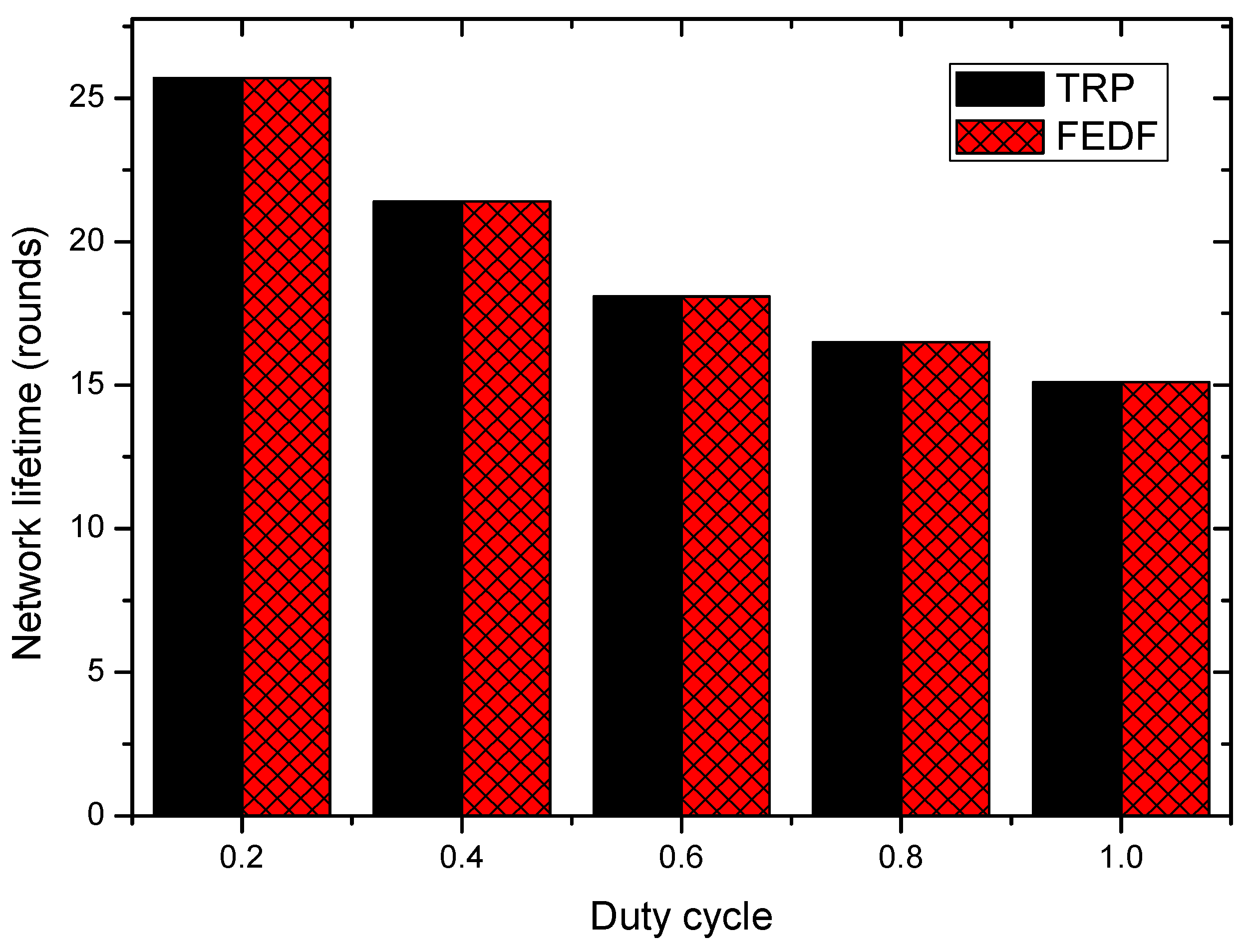
Figure 14 shows the network lifetime in the FEDF scheme and the TRP scheme under different duty cycles. In the FEDF scheme, the routing path is updated all the time, so every time the node has not yet reached its lifetime it will be replaced. Therefore, the entire network is in a dynamic process; its lifetime will not change.
6. Experimental Results
In this section, we will analyze the performance of the FEDF Scheme through specific examples. Assume that a mobile target keeps moving in the network, and every time the node senses the mobile target, it will send data to the sink. In the scheme, the routing path is changing dynamically with the movement of the target. The FEDF scheme is far superior to the traditional routing scheme of re-creating a path every time via analysis.
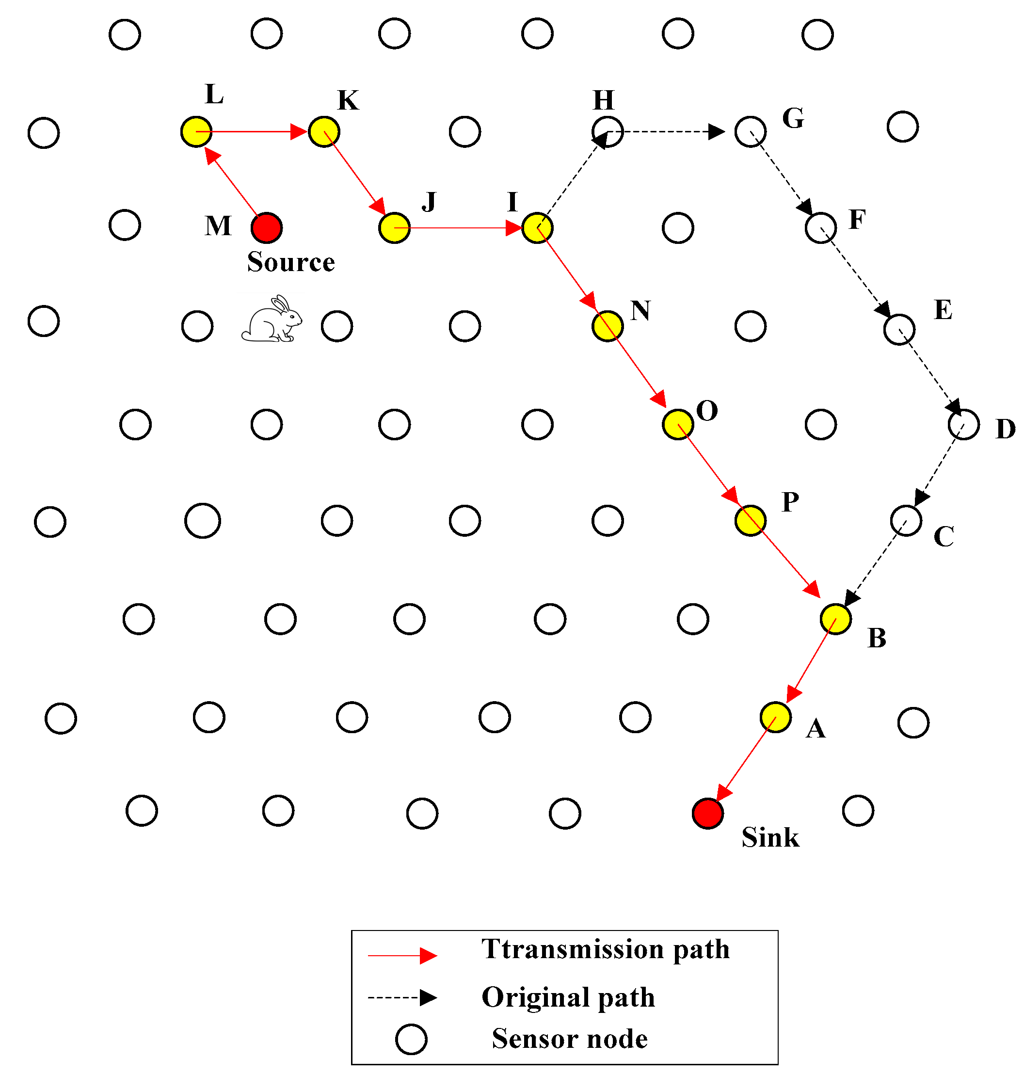
In the wireless sensor network, when the mobile target moves from the sink to node I, as shown in Figure 15, we detect possible EDP of a shortcut according to Algorithms 4 and 5. In addition, the value of path simplification coefficient λ is 1.5 through calculation.
At this time, according to Formula (25), in the example, the value of , are 0.7, 0.3 respectively, the calculation process is as shown in the table below. In the table, CCP stands for the cost of creating a path, including the delay and energy consumption. CSD stands for the cost of transmitting data through the existing path. TC stands for the total cost, which is the sum of the first two items in corresponding proportion. In addition, the unit of delay is ms, the unit of energy consumption is mJ.
In general, there is little possibility that the node near the sink is the EDP. According to Algorithm 4, η is set to 2. So the sink, node A, B, C, D, E, and F are pEDPs. Obviously, as is shown in Table 3; node B has the minimum cost, which is about 168.48. So it is selected as EDP. In addition, then the original path I→H→G→F→E→D→C→B, the target continues moving.
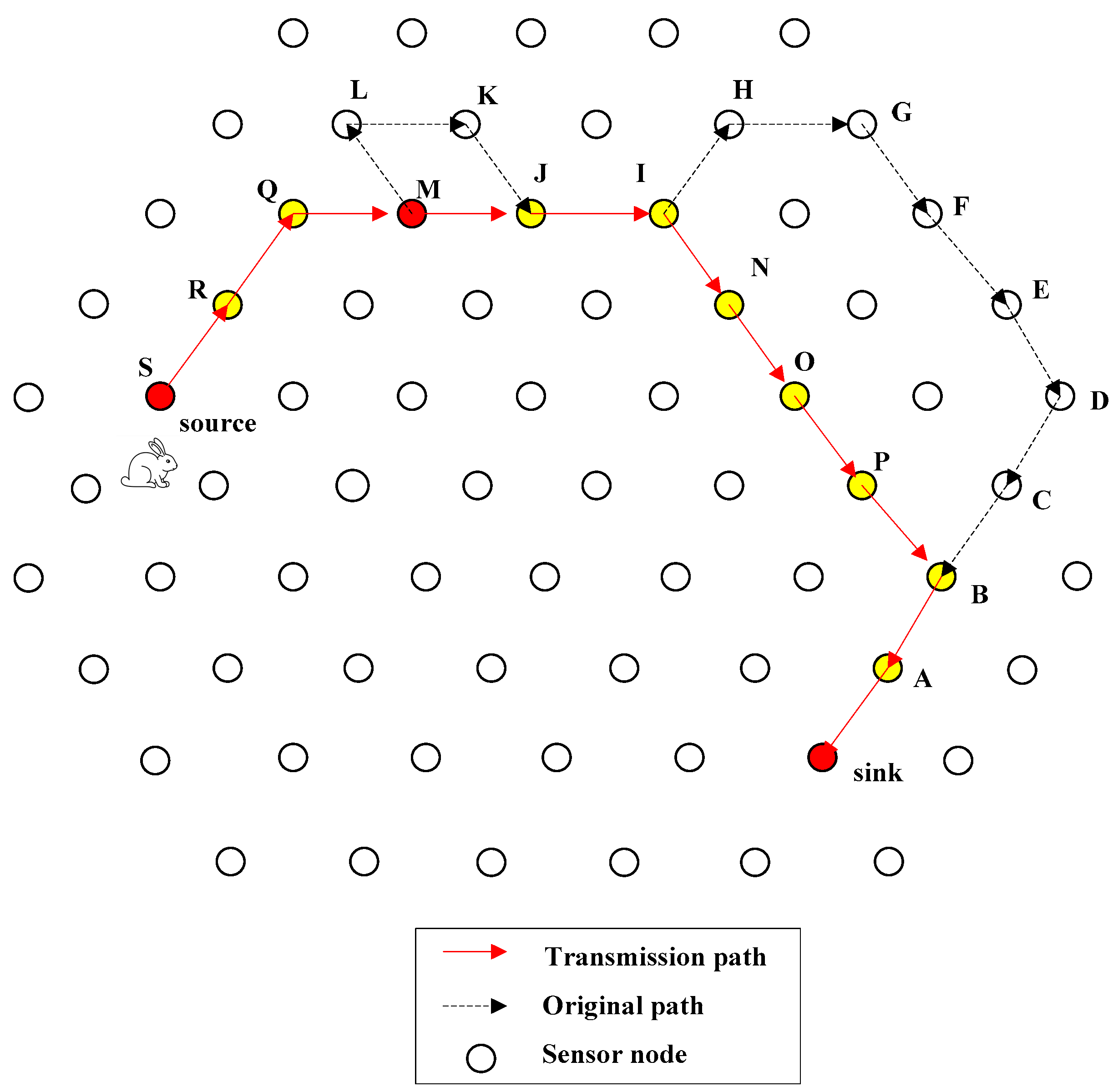
When the mobile target moves to node M, as is shown in Figure 16, the possible EDP is detected according to algorithms. In addition, we choose node J as EDP finally through calculation. In this case, the value of λ is 1.67.
The detailed calculation process is shown in the following Table 4. Node J, I, N, O, P, B, and A are pEDPs. If we choose node I as the EDP, hopCount from source to I is 2, hopCount from source to J is 1. It is easy to see that choosing J as the EDP costs less. So we do not include node I in the following table. As is shown in the table below, the total cost is minimal when node J is the EDP. The value is 171.74.
And after a while, the mobile target moves to node S, as is shown in Figure 17. Possible EDPs are detected according to algorithm. Node O is the final EDP through calculation. In addition, the value of path simplification coefficient λ is 1.57.
According to Algorithm 4, node M, J, I, N, O, P, B, and A are pEDPs. However, for nodes M, J, and I, the minimum hops from them to the source is the same as the hops of their original transmission path, and taking the original path eliminates the cost of re-creating a path, which has higher efficiency. The detailed calculating process is as shown in Table 5. Obviously, taking the original path costs less than choosing any node in the visited_list as the EDP for shortcuts. Therefore, we will not update the path this time.
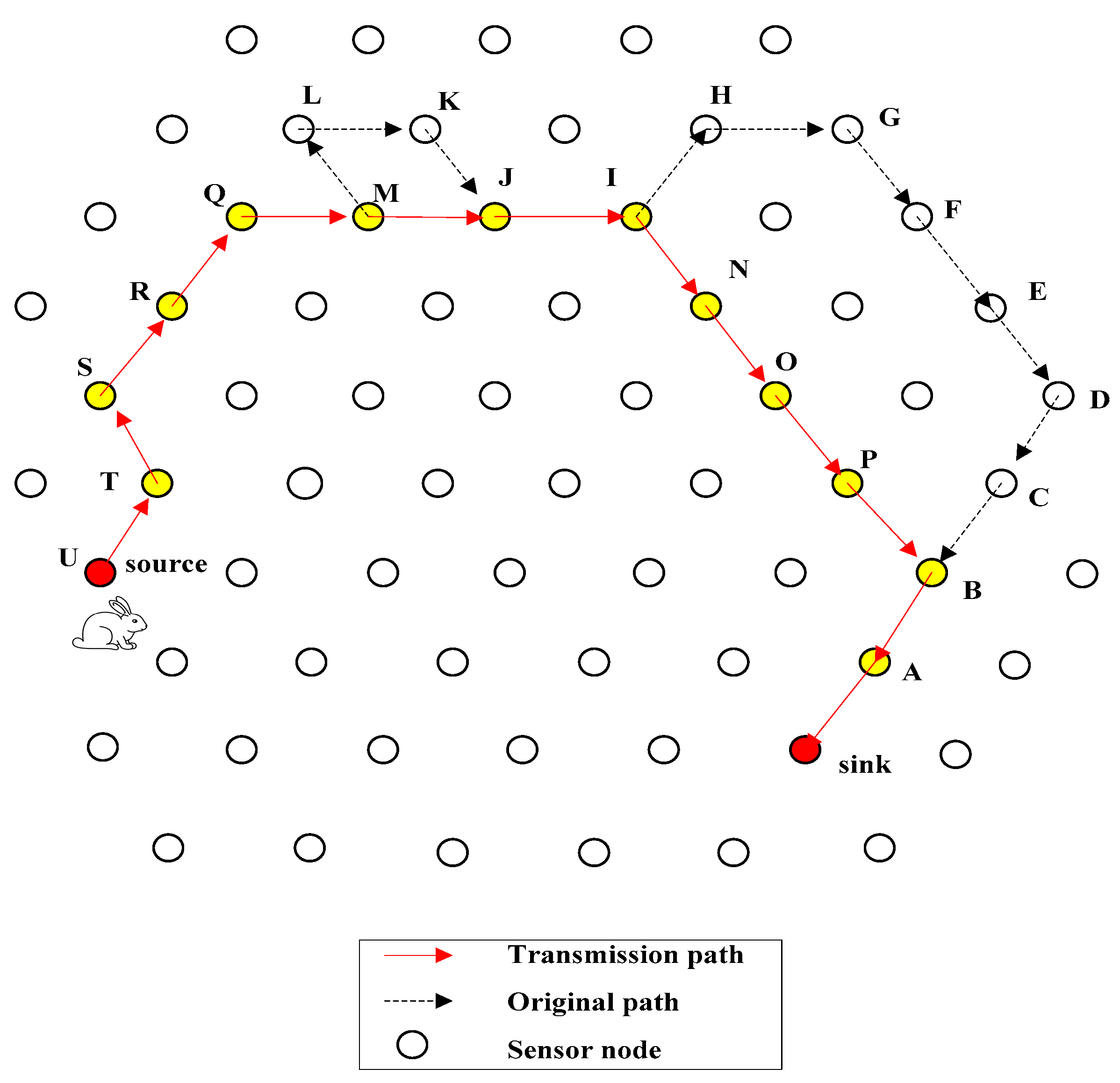
When the mobile target moves to node U as shown in Figure 18, nodes detected possible EDPs, and we choose the sink as the EDP finally through calculation—that is, we can create a path directly to the sink. At this moment, the routing path is close to a straight line, as is shown in Figure 19. The value of λ is 2.17 through calculation.
According to Algorithm 4, node R, Q, M, J, I, N, O, P, B, and A are pEDPs, because the minimum hops from source to node R or Q or M is the same as the original path; taking the original path will certainly cost less. There is no possibility that they are the EDP, so we do not include these three nodes in the calculation. The detailed process is shown in Table 6. When the sink is the EDP, the total cost is the minimum, which is 212.84.
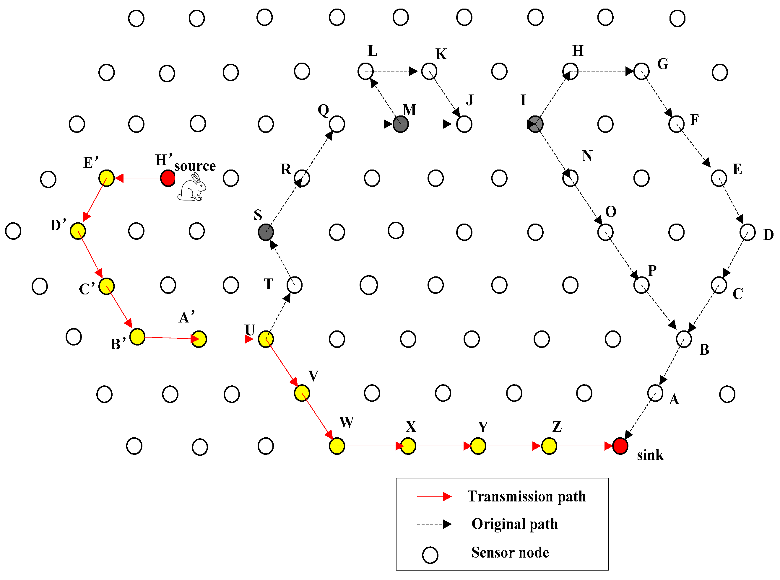
When the mobile target moves to node H’, as Figure 20 shows, according to Algorithm 4, possible EDPs are found. Finally, node U is selected as the EDP. In addition, λ is 1.33 at this moment.
Because we have already got the straight path U→V→W→X→Y→Z→sink, and it is the most efficient way to transmit directly through this route when data is in the position of node U, then we just need to consider node U, A’, B’ and C’ in the visited_list. The detailed process is shown in Table 7. When node U is EDP, the total cost is minimum, which is 212.79. In addition, the updated transmission path is shown in Figure 21.
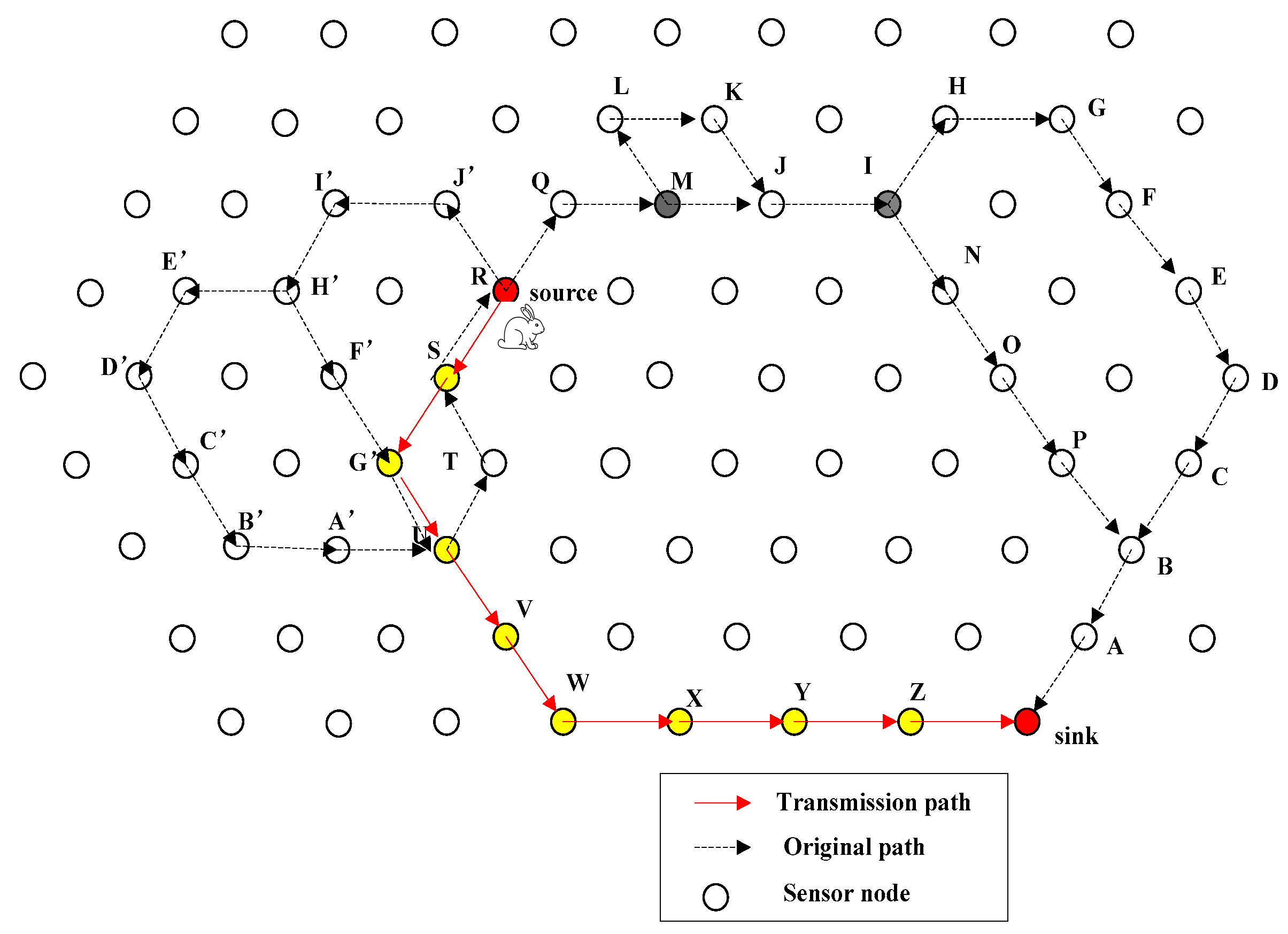
In the end, the mobile target moves to node R, which is shown in Figure 22. Node G’ is selected as the EDP through calculation. In addition, the value of λ is 1.71.
The detailed calculating process is shown in Table 8, when choosing node G’ as EDP, the total cost is minimum.
In the end, the transmission path is shown in Figure 23.
6.1. Transmission Delay
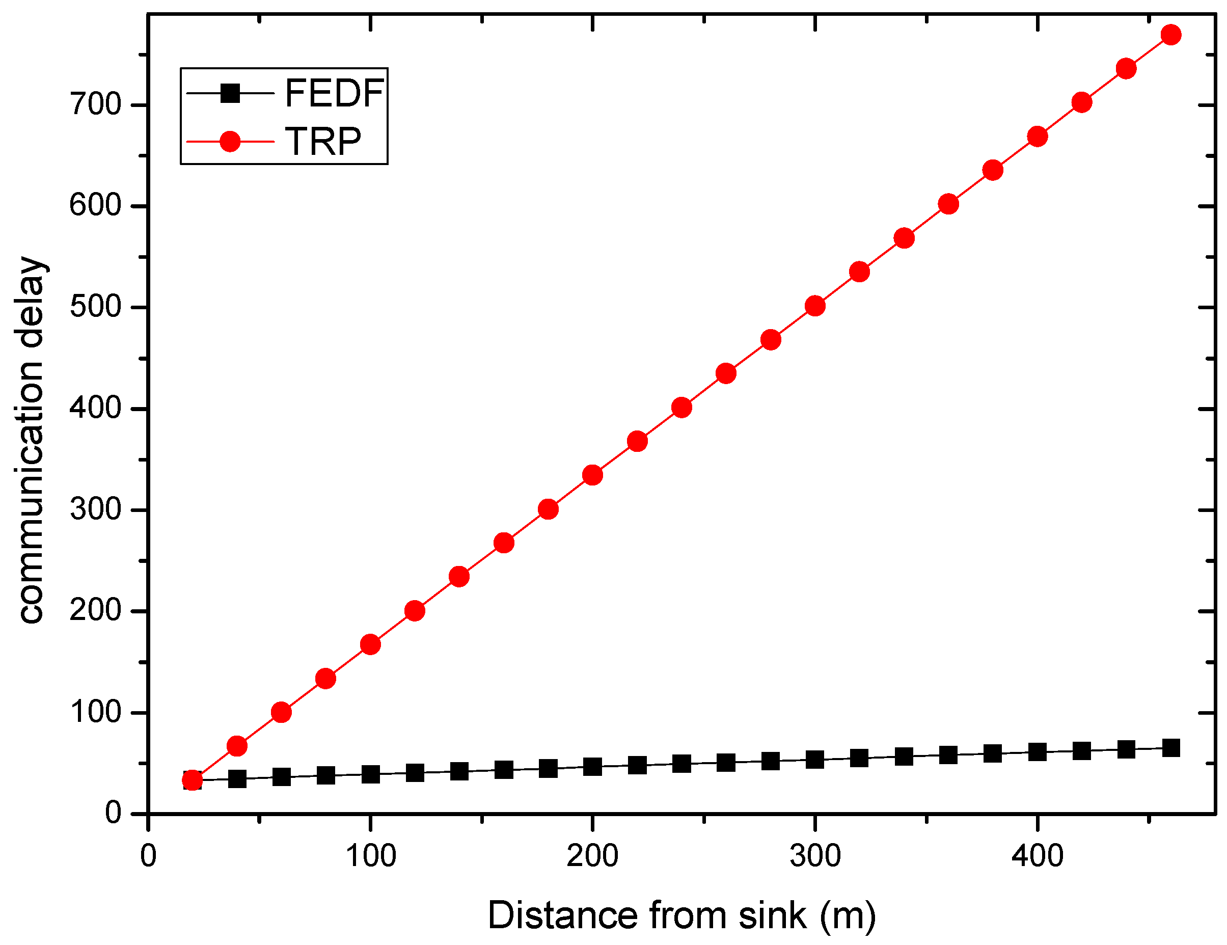
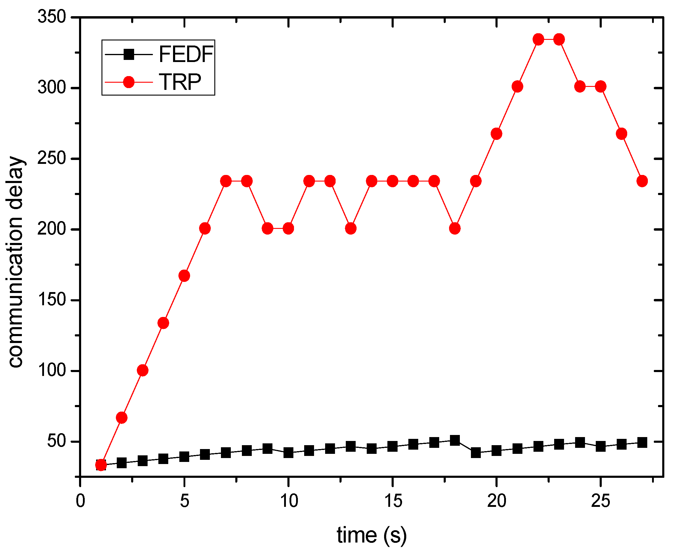
Figure 24 shows the communication delay in the FEDF scheme and traditional routing path (TRP) scheme. Assuming that the mobile target moves at 1 hop/s, the communication delay of two schemes presents a completely different performance as time grows. The target transmits data directly to the sink in the TRP scheme, so the node in this routing path may be in the state of sleep, which will waste a lot of time. In addition, the communication delay in the TRP scheme is in direct proportion to distance from sink. However, in the FEDF scheme, we adopt a QRR path, which will reduce delay significantly. Furthermore, we update the routing path in a timely manner, according to the algorithm, which will also help to reduce delay.
6.2. Energy Consumption
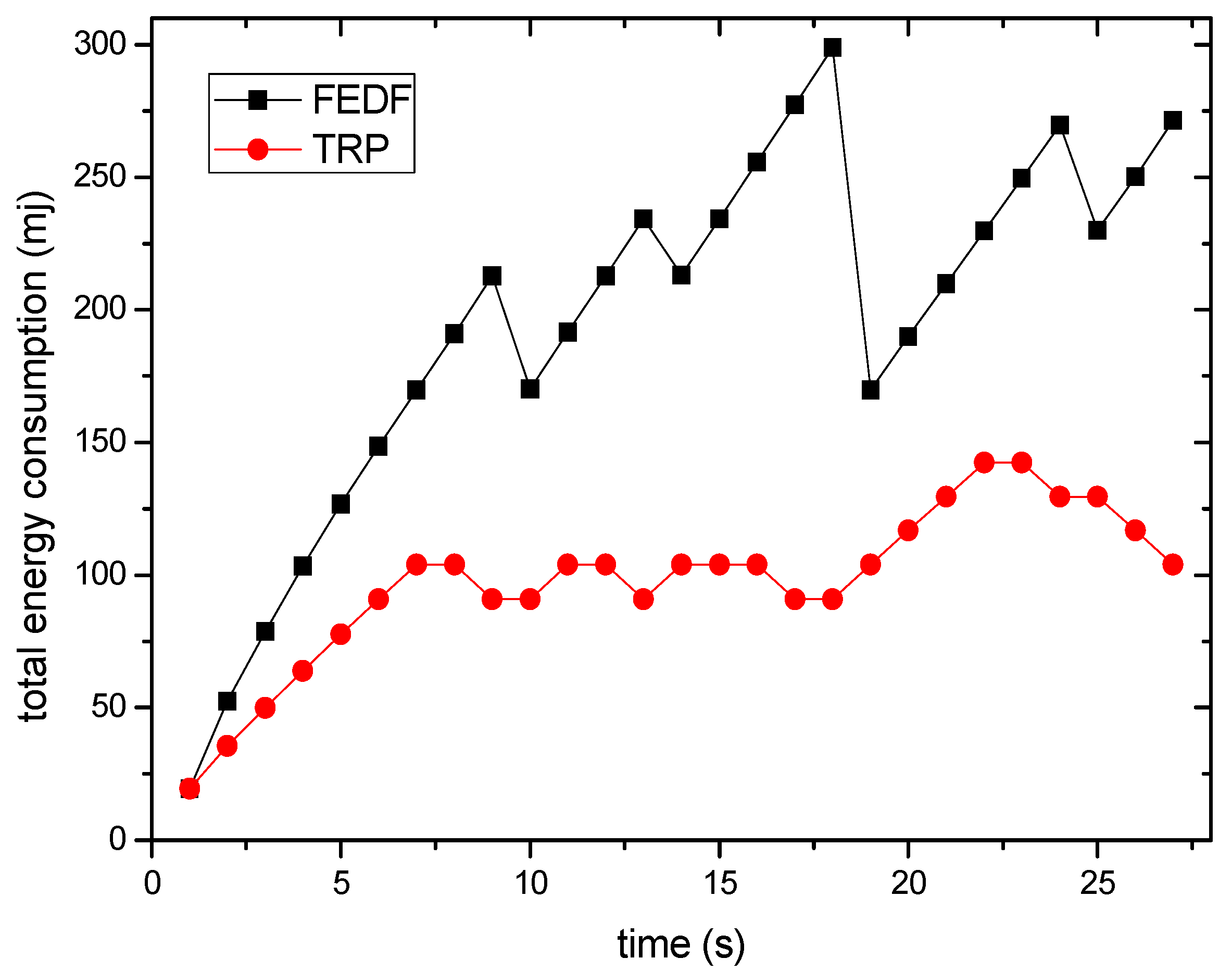
Figure 25 shows the energy consumption in the FEDF scheme and the TRP scheme. Energy consumption in the FEDF scheme is larger than that in the TRP scheme, because most nodes have high duty cycle. However, duty cycle of the node near sink is normal so as to maintain a relatively high network lifetime.
6.3. Path Length
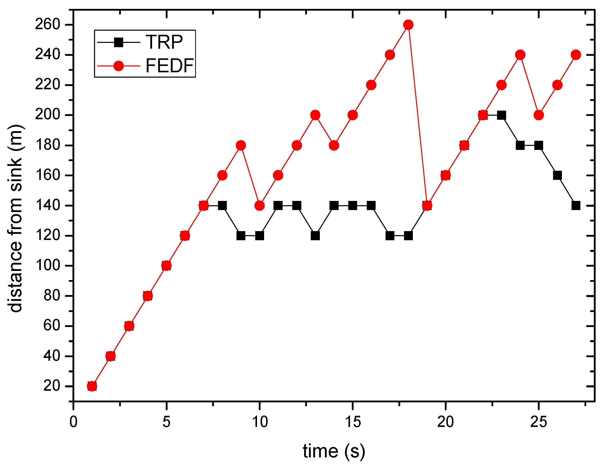
As is shown in Figure 26, the path length in the FEDF scheme is roughly an increasing trend, while in the TRP scheme it is directly related to the distance from sink.
7. Conclusions
In the sensor network, the node adopts the work/sleep working mode, and the end-to-end delay of data transmission from target to sink (communication delay) has a great influence on the transmission efficiency of the whole network. In a traditional scheme, the communication delay is quite large, which can waste a lot of resources. Therefore, we proposed the FEDF scheme in this paper. In the FEDF scheme, the duty cycle of nodes on a Quickly Reacted Routing (QRR) path and farther away from the sink is set to 1. Therefore, the sensing delay of each node is reduced, and the communication delay will reduce greatly. In the dynamic process of target moving, we analyze the cost of a shortcut, including the delay and energy consumption to update the routing path, and finally choose a path with relatively low cost. Comprehensive performance analysis shows that the FEDF scheme has outstanding performance both in delay and in energy utilization. Compared to a traditional routing scheme, it can reduce communication delay by 87.4%, improve network energy utilization by 2.65%, and ensure an increased network lifetime.
Acknowledgments
This work was supported in part by the National Natural Science Foundation of China (61772554, 61379110, 61370229 and 61370178), the National Basic Research Program of China (973 Program) (2014CB046305), the science and technology Projects of Guangdong Province, China (2016B010109008, and 2016B030305004), and the science and technology Projects of Guangzhou Municipality, China (201604010003, 201604016019).
Author Contributions
Mi Zhou designed the algorithms and wrote part of the manuscript. Ming Zhao commented the work. Anfeng Liu conceived of the work and wrote part of the manuscript. Ming Ma, Tian Wang and Changqin Huang commented the work.
Conflicts of Interest
The authors declare no conflict of interest.
References
- Kim, M.S.; Lee, J.K.; Park, J.H.; Kang, J.H. Security Challenges in Recent Internet Threats and Enhanced Security Service Model for Future IT Environments. J. Internet Technol. 2016, 17, 947–955. [Google Scholar]
- Kim, H.W.; Park, J.H.; Jeong, Y.S. Efficient Resource Management Scheme for Storage Processing in Cloud Infrastructure with Internet of Things. Wirel. Pers. Commun. 2016, 91, 1635–1651. [Google Scholar] [CrossRef]
- Liu, A.; Zhang, Q.; Li, Z.; Choi, Y.J.; Li, J.; Komuro, N. A green and reliable communication modeling for industrial internet of things. Comput. Electr. Eng. 2017, 58, 364–381. [Google Scholar] [CrossRef]
- Park, J.H.; Chao, H.C. Advanced IT-Based Future Sustainable Computing. Sustainability 2017, 9, 757. [Google Scholar] [CrossRef]
- Liu, A.; Chen, Z.; Xiong, N. An adaptive virtual relaying set scheme for loss-and-delay sensitive WSNs. Inform. Sci. 2018, 424, 118–136. [Google Scholar] [CrossRef]
- Liu, X.; Liu, Y.; Song, H.; Liu, A. Big data orchestration as a service networking. IEEE Commun. Mag. 2017, 55, 94–101. [Google Scholar]
- Wang, J.; Liu, A.; Zhang, S. Key parameters decision for cloud computing: Insights from a multiple game model. Concurr. Comput. Pract. Exp. 2017. [Google Scholar] [CrossRef]
- Su, Z.; Xu, Q.; Fei, M.; Don, M. Game Theoretic Resource Allocation in Media Cloud with Mobile Social Users. IEEE Trans. Multimed. 2016, 18, 1650–1660. [Google Scholar] [CrossRef]
- Li, H.; Liu, D.; Dai, Y.; Luan, T.H. Engineering searchable encryption of mobile cloud networks: When QoE meets QoP. IEEE Wirel. Commun. 2015, 22, 74–80. [Google Scholar] [CrossRef]
- Liu, Y.; Liu, A.; Guo, S.; Li, Z.; Choi, Y.J.; Sekiya, H. Context-aware collect data with energy efficient in Cyber-physical cloud systems. Future Gener. Comput. Syst. 2017. [Google Scholar] [CrossRef]
- Zhang, Q.; Liu, A. An unequal redundancy level based mechanism for reliable data collection in wireless sensor networks. EURASIP J. Wirel. Commun. Netw. 2016, 258, 1–22. [Google Scholar] [CrossRef]
- Liu, X.; Dong, M.; Ota, K.; Yang, L.T.; Liu, A. Trace malicious source to guarantee cyber security for mass monitor critical infrastructure. J. Comput. Syst. Sci. 2016. [Google Scholar] [CrossRef]
- Liu, X.; Zhao, S.; Liu, A.; Xiong, N.; Vasilakos, A.V. Knowledge-aware Proactive Nodes Selection Approach for Energy management in Internet of Things. Future Gener. Comput. Syst. 2017. [Google Scholar] [CrossRef]
- Liu, A.; Liu, X.; Wei, T.; Yang, L.T.; Rho, S.C.; Paul, A. Distributed Multi-representative Re-Fusion approach for Heterogeneous Sensing Data Collection. ACM Trans. Embed. Comput. Syst. 2017, 16, 73. [Google Scholar] [CrossRef]
- He, S.; Shin, D.; Zhang, J.; Chen, J.; Sun, Y. Full-view area coverage in camera sensor networks: Dimension reduction and near-optimal solutions. IEEE Trans. Veh. Technol. 2016, 65, 7448–7461. [Google Scholar] [CrossRef]
- Chen, X.; Ma, M.; Liu, A. Dynamic power management and adaptive packet size selection for IoT in e-Healthcare. Comput. Electr. Eng. 2017. [Google Scholar] [CrossRef]
- Chen, X.; Xu, Y.; Liu, A. Cross layer design for optimal delay, energy efficiency and lifetime in body sensor networks. Sensors 2017, 17, 900. [Google Scholar] [CrossRef] [PubMed]
- Xu, Y.; Chen, X.; Liu, A.; Hu, C. A latency and coverage optimized data collection scheme for smart cities based on vehicular ad-hoc networks. Sensors 2017, 17, 888. [Google Scholar] [CrossRef] [PubMed]
- Xu, Y.; Liu, A.; Huang, C. Delay-aware program codes dissemination scheme in Internet of everything. Mob. Inform. Syst. 2016. [Google Scholar] [CrossRef]
- Li, T.; Liu, Y.; Gao, L.; Liu, A. A Cooperative-based Model for Smart-Sensing Tasks in Fog Computing. IEEE Access 2017. [Google Scholar] [CrossRef]
- Chen, Z.; Liu, A.; Li, Z.; Choi, Y.J.; Sekiya, H.; Li, J. Energy-efficient broadcasting scheme for smart industrial wireless sensor networks. Mob. Inform. Syst. 2017, 2017, 7538190. [Google Scholar] [CrossRef]
- He, S.; Chen, J.; Li, X.; Shen, X.S.; Sun, Y. Mobility and intruder prior information improving the barrier coverage of sparse sensor networks. IEEE Trans. Mob. Comput. 2014, 13, 1268–1282. [Google Scholar]
- Zhao, S.; Liu, A. High performance target tracking scheme with low prediction precision requirement in WSNs. Int. J. Ad Hoc Ubiquitous Comput. 2017, in press. [Google Scholar]
- Chi, Y.P.; Chang, H.P. A tracking-assisted routing scheme for wireless sensor networks. Wirel. Pers. Commun. 2013, 70, 411–433. [Google Scholar] [CrossRef]
- Hu, Y.; Dong, M.; Ota, K.; Liu, A.; Guo, M. Mobile Target Detection in Wireless Sensor Networks with Adjustable Sensing Frequency. IEEE Syst. J. 2016, 10, 1160–1171. [Google Scholar] [CrossRef]
- Liu, A.; Liu, X.; Tang, Z.; Yang, L.T.; Shao, Z. preserving smart sink location privacy with delay guaranteed routing scheme for WSNs. ACM Trans. Embed. Comput. Syst. 2017, 16, 68. [Google Scholar] [CrossRef]
- Chen, Z.; Liu, A.; Li, Z.; Choi, Y.J.; Li, J. Distributed Duty cycle control for delay improvement in wireless sensor networks. Peer-to-Peer Netw. Appl. 2017, 10, 559–578. [Google Scholar] [CrossRef]
- Liu, X.; Li, G.; Zhang, S.; Liu, A. Big program code dissemination scheme for emergency software-define wireless sensor networks. Peer-to-Peer Netw. Appl. 2017. [Google Scholar] [CrossRef]
- Liu, Y.; Liu, A.; Li, Y.; Li, Z.; Choi, Y.J.; Sekiya, H.; Li, J. APMD: A fast data transmission protocol with reliability guarantee for pervasive sensing data communication. Pervasive Mob. Comput. 2017. [Google Scholar] [CrossRef]
- Huang, C.; Ma, M.; Liu, Y.; Liu, A. Preserving source location privacy for energy harvesting WSNs. Sensors 2017, 17, 724. [Google Scholar] [CrossRef] [PubMed]
- Gui, J.; Zhou, K. Flexible Adjustments between Energy and Capacity for Topology Control in Heterogeneous Wireless Multi-Hop Networks. J. Netw. Syst. Manag. 2016, 24, 789–812. [Google Scholar] [CrossRef]
- Liu, Q.; Liu, A. On the hybrid using of unicast-broadcast in wireless sensor networks. Comput. Electr. Eng. 2017. [Google Scholar] [CrossRef]
- Liu, X.; Liu, A.; Li, Z.; Tian, S.; Choi, Y.J.; Sekiya, H.; Li, J. Distributed cooperative communication nodes control and optimization reliability for resource-constrained WSNs. Neurocomputing 2017. [Google Scholar] [CrossRef]
- Chen, Z.; Ma, M.; Liu, X.; Liu, A.; Zhao, M. Reliability Improved Cooperative Communications over Wireless Sensor Networks. Symmetry 2017, 9, 209. [Google Scholar] [CrossRef]
- Wang, J.; Liu, A.; Yan, T.; Zeng, Z. A resource allocation model based on double-sided combinational auctions for transparent computing. Peer-to-Peer Netw. Appl. 2017. [Google Scholar] [CrossRef]
- Su, Z.; Xu, Q.; Zhu, H.; Wang, Y. A novel design for content delivery over software defined mobile social networks. IEEE Netw. 2015, 29, 62–67. [Google Scholar] [CrossRef]
- Li, T.; Liu, A.; Huang, C. A similarity scenario-based recommendation model with small disturbances for unknown items in social networks. IEEE Access 2016, 4, 9251–9272. [Google Scholar] [CrossRef]
- Zhou, S.; Xu, Q. Content distribution over content centric mobile social networks in 5G. IEEE Commun. Mag. 2015, 53, 66–72. [Google Scholar] [CrossRef]
- Liu, X.; Liu, A.; Huang, C. Adaptive Information Dissemination Control to Provide Diffdelay for Internet of Things. Sensors 2017, 17, 38. [Google Scholar] [CrossRef] [PubMed]
- Asudeh, A.; Zaruba, G.V.; Das, S.K. A general model for MAC protocol selection in wireless sensor networks. Ad Hoc Netw. 2016, 36, 189–202. [Google Scholar] [CrossRef]
- Feng, X.; Wang, Z.; Liu, X.; Liu, J. ADCNC-MAC: Asynchronous duty cycle with network-coding MAC protocol for underwater acoustic sensor networks. EURASIP J. Wirel. Commun. Netw. 2015, 2015, 207. [Google Scholar] [CrossRef]
- Bakshi, M.; Kaddour, M.; Jaumard, B.; Narayanan, L. An efficient method to minimize TDMA frame length in wireless sensor networks. In Proceedings of the 2015 IEEE Wireless Communications and Networking Conference (WCNC), New Orleans, LA, USA, 9–12 March 2015; pp. 825–830. [Google Scholar]
- Gao, D.; Wu, G.; Liu, Y.; Zhang, F. Bounded end-to-end delay with Transmission Power Control techniques for rechargeable wireless sensor networks. AEU Int. J. Electron. Commun. 2014, 68, 396–405. [Google Scholar] [CrossRef]
- Merlin, C.J.; Heinzelman, W.B. Duty cycle control for low-power-listening MAC protocols. IEEE Trans. Mob. Comput. 2010, 9, 1508–1521. [Google Scholar] [CrossRef]
- Sun, Y.; Du, S.; Johnson, D.B.; Gurewitz, O. DW-MAC: A low latency, energy efficient demand—Wakeup MAC protocol for wireless sensor networks. In Proceedings of the 9th ACM International Symposium on Mobile ad Hoc Networking and Computing, Hong Kong, China, 26–30 May 2008; pp. 53–62. [Google Scholar]
- Zhao, Y.Z.; Ma, M.; Miao, C.Y.; Nguyen, T.N. An energy-efficient and low-latency MAC protocol with adaptive scheduling for multi-hop wireless sensor networks. Comput. Commun. 2010, 33, 1452–1461. [Google Scholar] [CrossRef]
- Xu, J.; Liu, X.; Ma, M.; Liu, A.; Wang, T.; Huang, C. Intelligent Aggregation based on Content Routing Scheme for Cloud Computing. Symmetry 2017, 9, 221. [Google Scholar] [CrossRef]
- Naveen, K.P.; Kumar, A. Relay selection for geographical forwarding in sleep-wake cycling wireless sensor networks. IEEE Trans. Mob. Comput. 2013, 12, 475–488. [Google Scholar] [CrossRef]
Figure 1.
The network model.
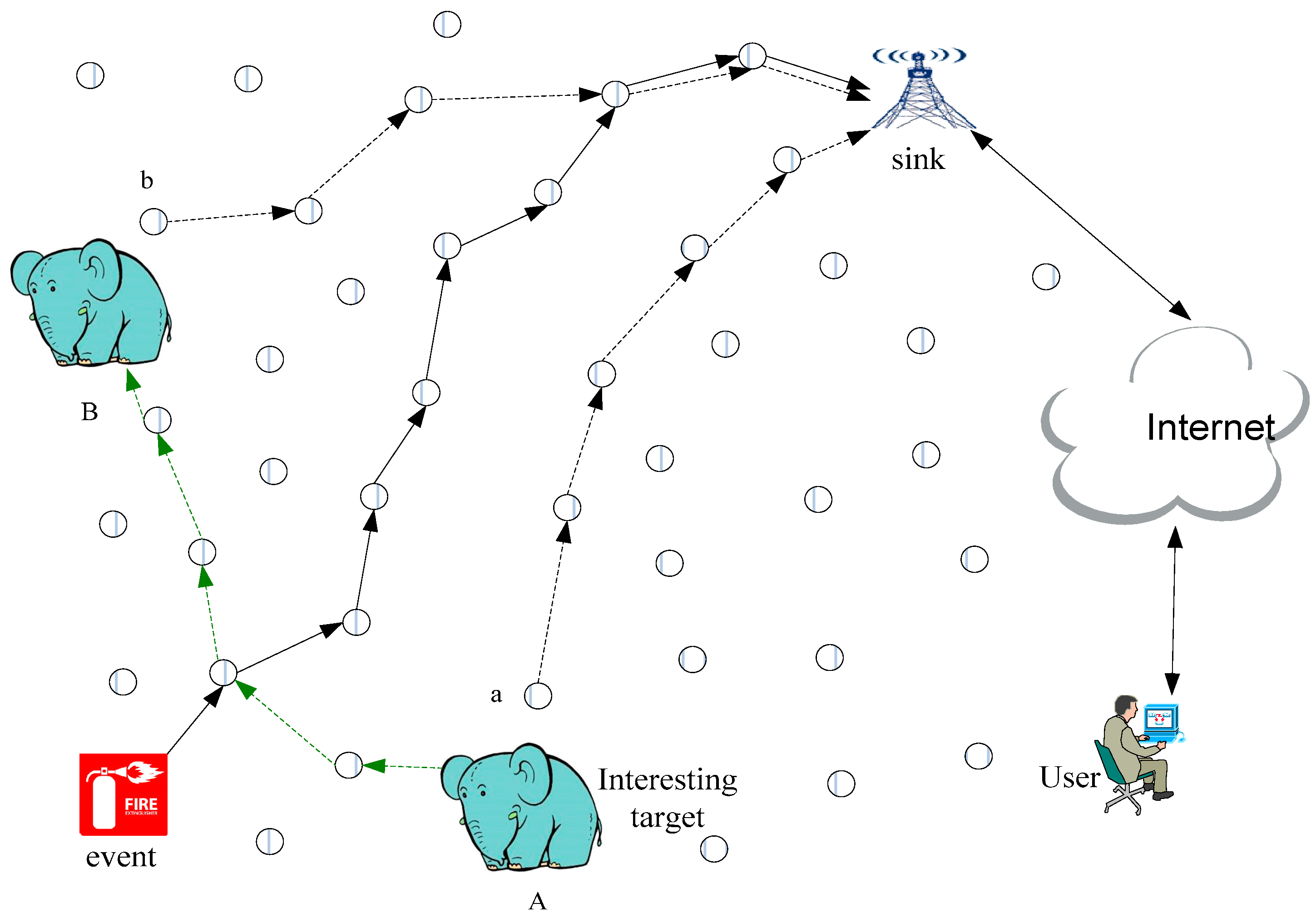
Figure 2.
The mobile target and sink network.
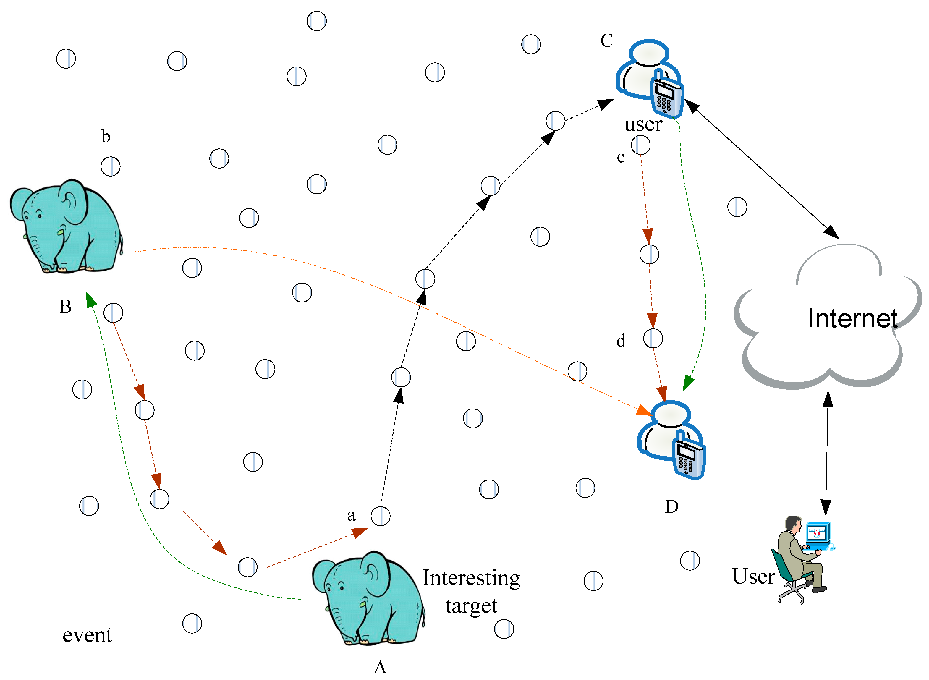
Figure 3.
Communication delay on normal path and QRR path.

Figure 4.
Communication delay on NP and QRRP under different duty cycles.
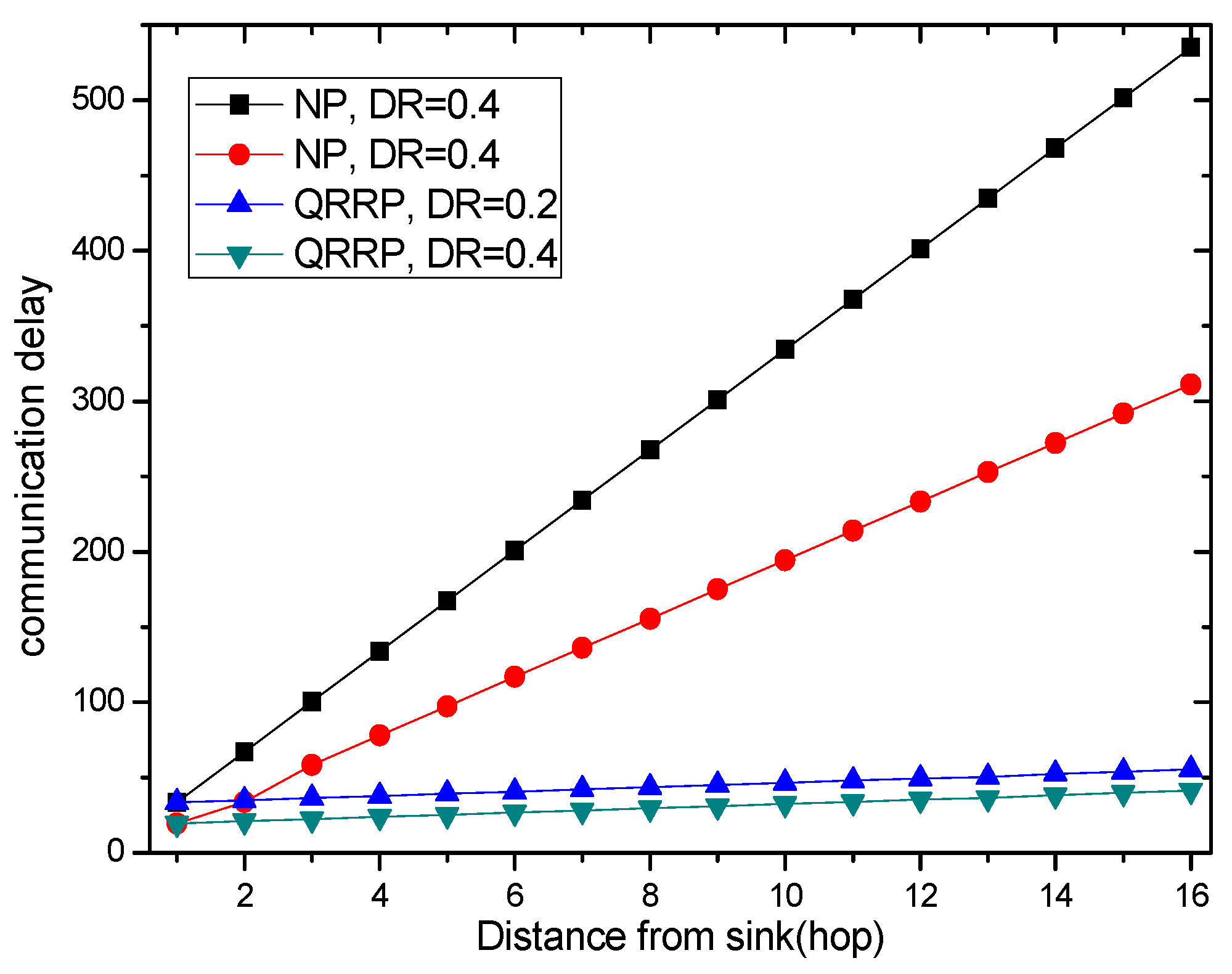
Figure 5.
General method for data transmission.
Figure 6.
Initialized network.

Figure 7.
Initial Quickly Reacted Routing Path.

Figure 8.
Possible shortcuts.

Figure 9.
End to end delay in FEDF and TRP.

Figure 10.
Communication delay in FEDF from different λ.
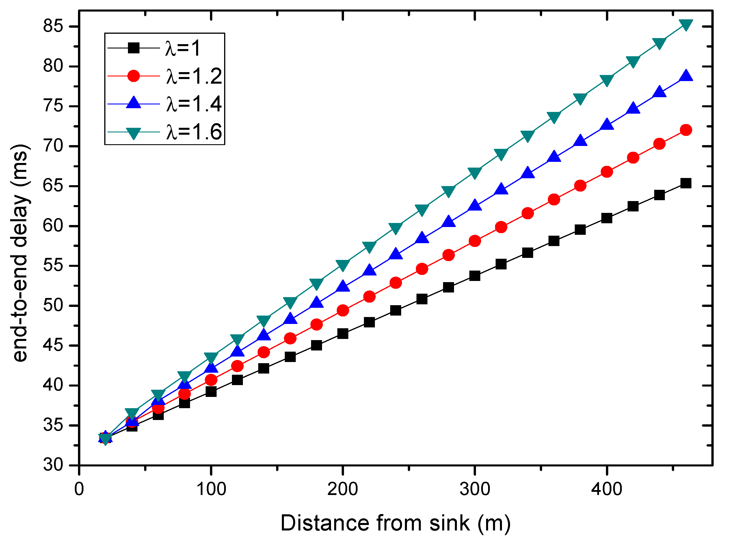
Figure 11.
Communication delay in FEDF from different λ and in TRP.

Figure 12.
The energy consumption in FEDF and TRP.

Figure 13.
Energy utilization in TRP and FEDF with different λ.
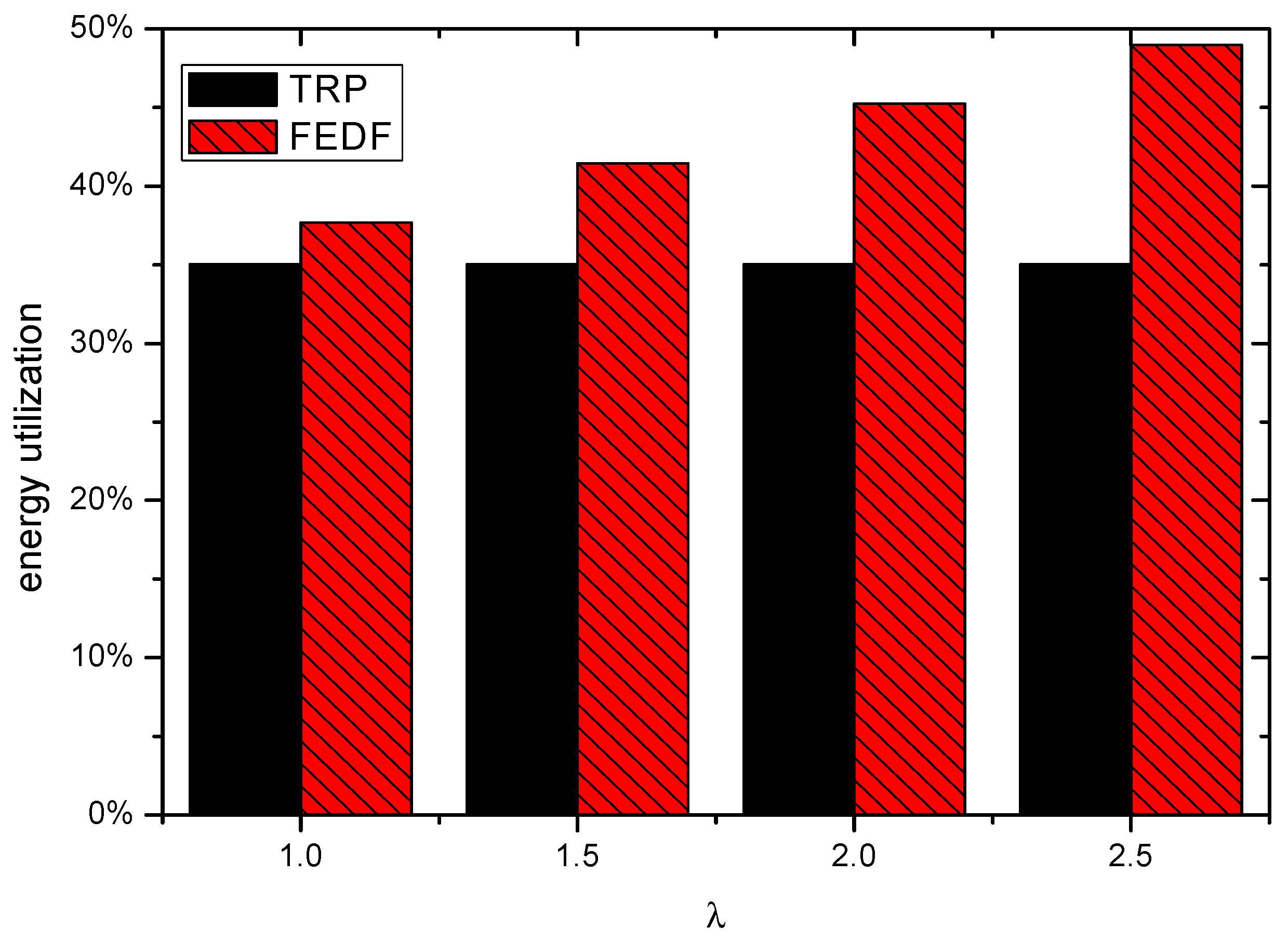
Figure 14.
Network lifetime in FEDF and TRP under different duty cycle.

Figure 15.
Transmission path when the first time possible shortcuts are detected.
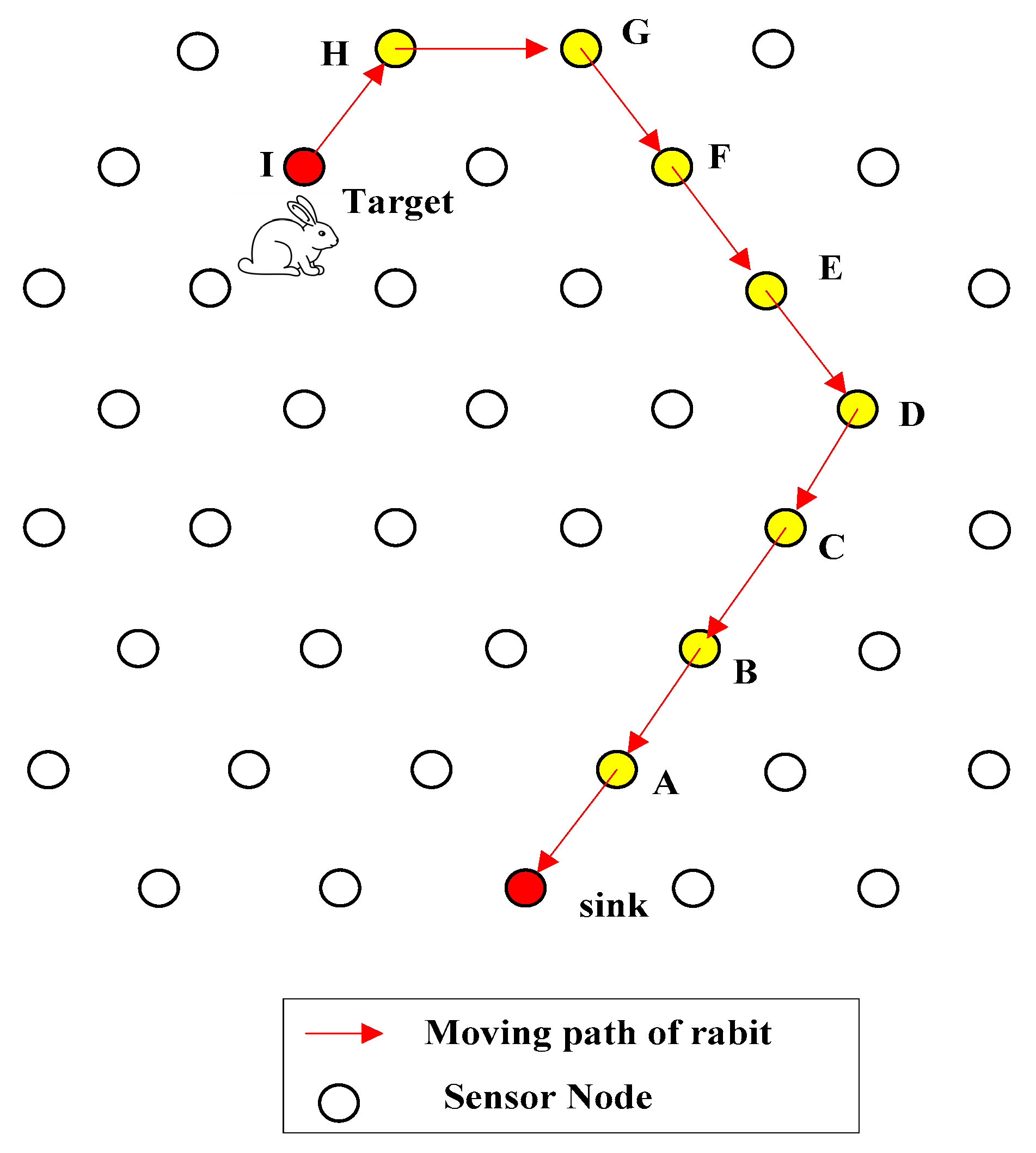
Figure 16.
Transmission path when the second time possible shortcuts are detected.

Figure 17.
Transmission path when the third time possible shortcuts are detected.

Figure 18.
Transmission path when the forth time possible shortcuts are detected.

Figure 19.
The updated transmission path from node U to sink.
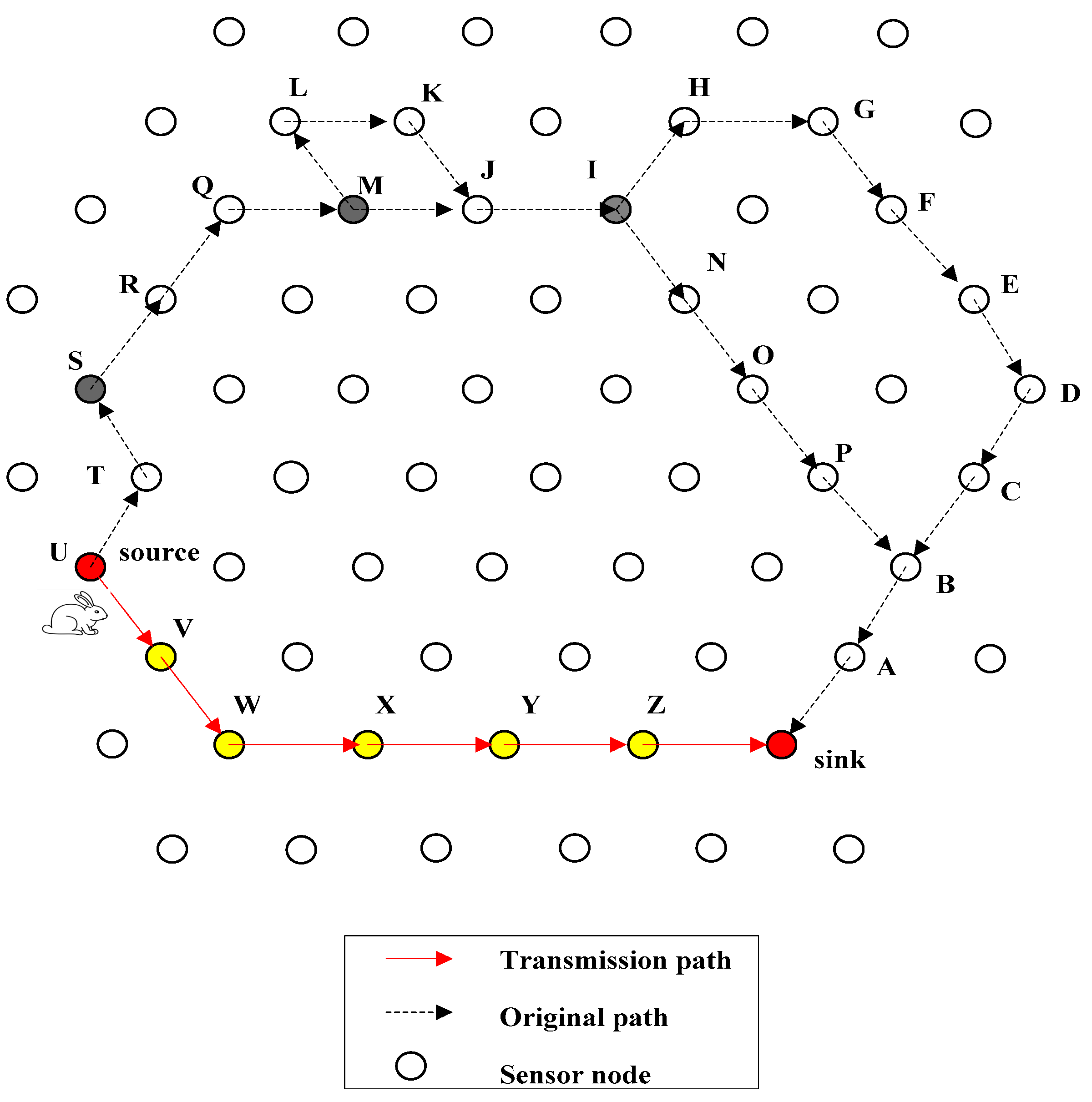
Figure 20.
Transmission path when the fifth time possible shortcuts are detected.

Figure 21.
The updated transmission path from node H’ to sink.
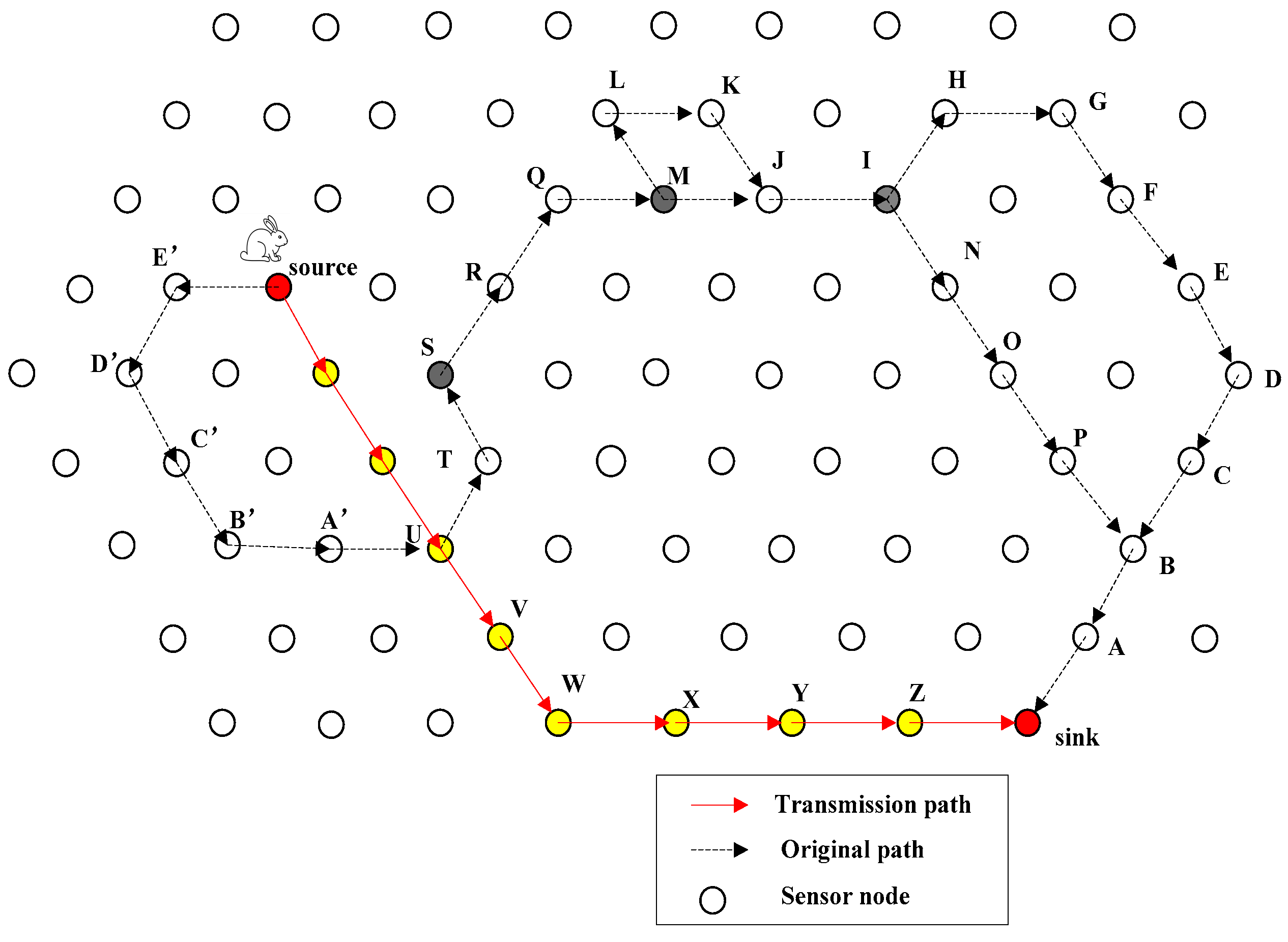
Figure 22.
Transmission path when the seventh time possible shortcuts are detected.
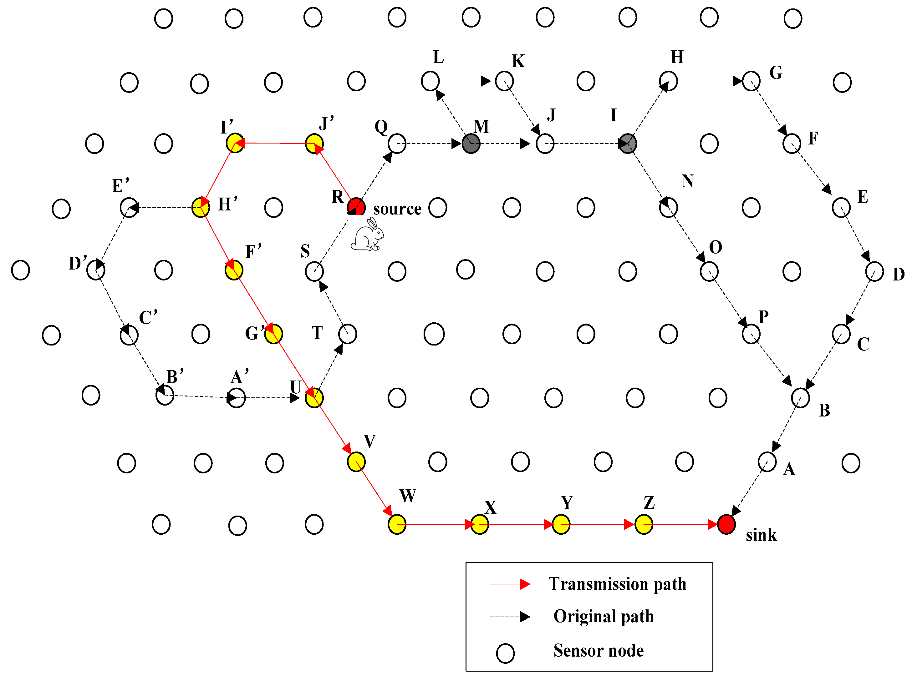
Figure 23.
The final transmission path.

Figure 24.
Communication delay in FEDF scheme and TRP scheme.

Figure 25.
Total energy consumption in FEDF scheme and TRP scheme.

Figure 26.
Distance from sink in FEDF Scheme and TRP Scheme.

Table 1.
Network Parameters.
| Parameter | Value | Description |
|---|---|---|
| 0.5 | Initial energy (J) | |
| 15 | Sensing duration (s) | |
| 100 | Communication duration (ms) | |
| 0.26 | Preamble duration (ms) | |
| 0.26 | Acknowledge window duration (ms) | |
| 0.93 | Data packet duration (ms) | |
| 0.0511 | Power consumption in transmission (w) | |
| 0.0588 | Power consumption in receiving (w) | |
| 0.0036 | Power consumption in sensing (w) | |
| 2.4 × 10⁻⁷ | Power consumption in sleeping (w) |
Table 2.
Parameters Related to Calculation.
| Symbol | Description |
|---|---|
| Sensing duty cycle | |
| Communication duty cycle | |
| Energy consumption in low power listening | |
| Energy consumption in data transmission | |
| Energy consumption in event sensing | |
| Energy consumption in data receiving |
Table 3.
Total cost (EDP is B).
| Cost/pEDP | Sink | A | B | C | D | E | F |
|---|---|---|---|---|---|---|---|
| CCP | 267.94 | 215.03 | 165.49 | 165.49 | 165.05 | 117.39 | 69.78 |
| CSD | 189.22 | 169.76 | 169.76 | 216.97 | 241.24 | 192.12 | 235.43 |
| TC | 212.84 | 183.34 | 168.48 | 201.52 | 218.38 | 169.70 | 185.74 |
Table 4.
Total cost (EDP is J).
| Cost/pEDP | J | A | N | O | P | B | Original |
|---|---|---|---|---|---|---|---|
| CCP | 23.10 | 267.94 | 117.39 | 165.05 | 213.33 | 264.57 | 0 |
| CSD | 235.43 | 210.04 | 239.15 | 241.24 | 244.71 | 258.20 | 280.90 |
| TC | 171.74 | 227.41 | 202.62 | 218.38 | 235.30 | 260.11 | 196.63 |
Table 5.
Total cost (the original is the best).
| Cost/pEDP | Sink | N | O | P | B | A | Original |
|---|---|---|---|---|---|---|---|
| CCP | 314.24 | 211.35 | 211.35 | 259.19 | 308.73 | 308.73 | 0 |
| CSD | 211.96 | 288.94 | 263.97 | 267.16 | 272.45 | 237.96 | 305.43 |
| TC | 242.64 | 265.66 | 248.18 | 264.77 | 283.34 | 259.19 | 213.80 |
Table 6.
Total cost (EDP is sink).
| Cost/pEDP | Sink | A | B | P | O | N | I | J |
|---|---|---|---|---|---|---|---|---|
| CCP | 267.94 | 267.94 | 264.57 | 264.57 | 262.87 | 260.730 | 259.59 | 211.67 |
| CSD | 189.22 | 210.14 | 258.20 | 285.95 | 305.21 | 321.69 | 340.28 | 335.30 |
| TC | 212.84 | 227.48 | 260.11 | 279.53 | 292.51 | 303.40 | 316.07 | 298.21 |
Table 7.
Total cost (EDP is U).
| Cost/pEDP | U | A’ | B’ | C’ | Original |
|---|---|---|---|---|---|
| CCP | 114.31 | 114.31 | 114.03 | 67.70 | 0 |
| CSD | 254.99 | 277.73 | 298.19 | 297.89 | 319.08 |
| TC | 212.79 | 228.71 | 242.94 | 228.83 | 223.36 |
Table 8.
Total cost (EDP is G’).
| Cost/pEDP | G’ | F’ | H’ | Original |
|---|---|---|---|---|
| CCP | 67.87 | 69.02 | 69.02 | 0 |
| CSD | 257.42 | 277.89 | 299.33 | 320.77 |
| TC | 201.16 | 215.23 | 230.24 | 224.54 |
© 2017 by the authors. Licensee MDPI, Basel, Switzerland. This article is an open access article distributed under the terms and conditions of the Creative Commons Attribution (CC BY) license (http://creativecommons.org/licenses/by/4.0/).
Share and Cite
MDPI and ACS Style
Zhou, M.; Zhao, M.; Liu, A.; Ma, M.; Wang, T.; Huang, C. Fast and Efficient Data Forwarding Scheme for Tracking Mobile Targets in Sensor Networks. Symmetry 2017, 9, 269. https://doi.org/10.3390/sym9110269
AMA Style
Zhou M, Zhao M, Liu A, Ma M, Wang T, Huang C. Fast and Efficient Data Forwarding Scheme for Tracking Mobile Targets in Sensor Networks. Symmetry. 2017; 9(11):269. https://doi.org/10.3390/sym9110269
Chicago/Turabian StyleZhou, Mi, Ming Zhao, Anfeng Liu, Ming Ma, Tiang Wang, and Changqin Huang. 2017. "Fast and Efficient Data Forwarding Scheme for Tracking Mobile Targets in Sensor Networks" Symmetry 9, no. 11: 269. https://doi.org/10.3390/sym9110269
Note that from the first issue of 2016, this journal uses article numbers instead of page numbers. See further details here.