An Appraisal Model Based on a Synthetic Feature Selection Approach for Students’ Academic Achievement

Abstract

Obtaining necessary information (and even extracting hidden messages) from existing big data, and then transforming them into knowledge, is an important skill. Data mining technology has received increased attention in various fields in recent years because it can be used to find historical patterns and employ machine learning to aid in decision-making. When we find unexpected rules or patterns from the data, they are likely to be of high value. This paper proposes a synthetic feature selection approach (SFSA), which is combined with a support vector machine (SVM) to extract patterns and find the key features that influence students’ academic achievement. For verifying the proposed model, two databases, namely, “Student Profile” and “Tutorship Record”, were collected from an elementary school in Taiwan, and were concatenated into an integrated dataset based on students’ names as a research dataset. The results indicate the following: (1) the accuracy of the proposed feature selection approach is better than that of the Minimum-Redundancy-Maximum-Relevance (mRMR) approach; (2) the proposed model is better than the listing methods when the six least influential features have been deleted; and (3) the proposed model can enhance the accuracy and facilitate the interpretation of the pattern from a hybrid-type dataset of students’ academic achievement.

1. Introduction

We are currently in the era of big data. Due to advanced technology and a diversified dissemination pipeline, our lives are full of all kinds of data which can be obtained easily. Big data are available for people to explore, query, and use. Moreover, the famous advertising line is confirmed: “We have everything you want and nothing strange.” However, the following questions arise: “Do I have the ability to use these data?”, “How can I find the information I want?”, and “In seemingly unrelated data, can I find hidden information?” [1]. Therefore, in this era, we must learn how to obtain the information we need, and even extract hidden messages from existing data, and then transform the information into knowledge [2].

Data mining technology has received increasing attention in recent years in various fields because of its extraordinary process [3]. Specifically, from a large amount of data, which may be incomplete or noisy, a fuzzy condition can find the hidden, regular, unknown information, which may be transformed to knowledge in the future. When we find unexpected information, it is likely to be of high value [4].

In developing good personality and learning strategies, the most important educational period for students is elementary school. This period should be considered when determining what factors influence students’ academic achievement and allow students to achieve balanced development. These two issues have been the focus of everyone’s attention. Therefore, the objectives of this study are defined as follows:

• The large amount of long-established data must reveal intrinsic patterns for the analysis to be highly valuable. Therefore, use data collected from elementary school to establish a feasible supervised learning model.
• Utilise a data mining technique and proposed feature selection approach to determine the key factors of students’ academic achievement from the vast amount of data.
• Find the differences between and properties of different algorithms, and provide the research results to educational and tutorship personnel for reference.

The remainder of this paper is organised as follows. Section 2 provides a review of the relevant literature, including the related factors in academic achievement, feature selection, and data mining techniques. Section 3 describes the proposed method and algorithm. The data analysis and results are presented in Section 4. The last section presents the conclusion.

2. Literature Review

This section introduces the related works, including the related factors in academic achievement, feature selection approaches, and data mining techniques.

2.1. Related Factors in Academic Achievement

Academic achievement is the result obtained through learning process behaviour, and the main scientific tool that we use to measure student academic achievement is commonly called the achievement test. The academic achievement test is a psychological test. After a teaching process, we usually use it to evaluate students’ learning achievement level [5]. Achievement was defined in [6] as follows:

• After the action, individuals or groups successfully achieve the goal that they set;
• In certain fields (disciplines), the attainment of various honours (such as awards and academic degrees);
• The scores that are obtained from the test of academic achievement or vocational achievement; and
• The scores in various subjects that students obtain in school.

Regarding related factors of academic achievement, early scholars [7] discovered two important key factors that affect the ability of individuals to achieve social status: “socio-economic status of parents” and “individual educational achievement”. However, the socio-economic status of parents is already established, and academic achievement is affected by not only by the parents’ socio-economic status, but also acquired environmental effects that cannot be ignored. Coleman [8] proposed that factors that affect academic achievement are related to the family environment and the individual student. Meighan and Bondi [9] indicated that parental attitudes to education, the child’s intelligence quotient, learning opportunities, etc., all influence academic achievement.

For convenient comparison and analysis, previous scholars’ discoveries regarding the factors of academic achievement are listed as follows:

• The four factors that affect academic achievement are attitude to education, living environment, value concept, and language type [10];
• Factors of academic achievement should be divided into internal and external factors. Internal factors involve intelligence, motivation, personality, and so on. External factors relate to teaching methods, type of learning groups individuals participate in, influence of teachers [11], and so on;
• According to [12], the main factors of academic achievement are individual psychological factors, physiological factors, and related environmental factors (family, school, society); and
• Parents affect students’ academic achievement through various factors, such as parenting style, educational values, educational beliefs, and family atmosphere [13].

According to many previous studies about academic achievement, the factors to which scholars often paid close attention, and that this study could collect in the related database and that this study focuses on, are listed in

Table 1. The factors of students’ academic achievement focused on in this study.

Scope	Coverage	Factor
student	personal aspects	Language average score
		Math average score
		Science average score
		Arts average score
		Social average score
		Physical average score
		Integrated activities average score
		Behaviour average score
environment	family aspects	Education levels of parents
		Occupations of parents
		Ages of parents
		Number of children
		Self-ranking
	school aspects	Teacher
	social aspects	Student Identity Background

.

2.2. Feature Selection

Feature selection, which is also known as “variable selection”, “attribute selection”, or “variable subset selection”, is the process of selecting a subset of relevant features (variables, predictors) for use in model construction. Feature selection techniques are used for the following reasons [14]:

• to reduce the dimension of the data and shorten the training times of algorithms;
• to enhance the operation effectively;
• to improve the accuracy of classification;
• to improve the generalisation ability and prevent overfitting; and
• for simplification of models, to make them easier to interpret by researchers and users.

The central premise when using a feature selection technique is that the data contain many features that are either redundant or irrelevant and can, thus, be removed without incurring much loss of information [15]. Redundant or irrelevant features are two distinct notions, since one relevant feature may be redundant in the presence of another relevant feature with which it is strongly correlated [16].

This research used five feature selection methods to synthesise feature selection as follows: multilayer perceptron (MLP), radial basis function (RBF), discriminant analysis (DA), cascade correlation network (CCN), and decision tree forest (DTF). These feature selection methods are introduced individually in the following subsections. In addition, for comparison with the proposed approach, the well-known feature selection approach called minimum-redundancy-maximum-relevance (mRMR) [17] was used.

2.2.1. Multilayer Perceptron (MLP)

MLP is an artificial network model. It is inspired by the operation of the human brain. Posner, along with cognitive scientists and neurologists, made efforts to understand the functioning of the human brain, in addition to constructing the neural network model of the human brain, and launched a series of simulation studies [18,19]. MLP is a feed-forward artificial neural network structure in which a set of input vectors are mapped into a set of output vectors. It can be viewed as a directed graph that consists of nodes composed of multiple layers, where each layer is fully connected to the next layer [20]. In addition to the input nodes, each node is a neuron with a non-linear activation function. The back-propagation algorithm of supervised learning methods is often used to train the MLP [21,22]. The MLP overcomes the weakness of the general perceptron that is related to the issue of linear inseparability [23].

If each neuron activation function is linear, the MLP can incorporate any number of layers into an equivalent reduction single sensor [20]. The MLP can use any form of activation function, such as a step function or logistic sigmoid function. However, to ensure that the back-propagation algorithm is effective in learning, the activation function must be differentiable. Thus, the hyperbolic tangent, sigmoid, and logistic sigmoid functions are frequently used as activation functions [24,25].

2.2.2. Radial Basis Function (RBF) Network

Broomhead and Lowe [26] proposed the RBF (radial basis function) network, which is also an artificial neural network. Its main characteristic is that it simulates the partial adjustment of the brain cortex axons; it also has good mapping capabilities. The basic architecture of RBF is the same as that of MLP: it has an input layer, output layer, and hidden layer, which form a feed-forward artificial neural network. This algorithm uses function approximation (curve fitting) to construct the network. The RBF network’s activation of hidden units is based on the distance between the input vector and a prototype vector [27,28,29]. In recent years, it has become a very popular algorithm due to its simple structure and high training efficiency.

This algorithm employs a two-stage form of learning: unsupervised learning is used to select a centre in the first stage and supervised learning is used to adjust the link weight vector in the next stage. The purpose of centre selection is to obtain a centre that achieves the required accuracy with a suitably sized network and initial values for the relevant parameters. Common centre selection methods are random, clustering, and supervised selection methods.

2.2.3. Discriminant Analysis (DA)

The DA algorithm is a statistical method. Its main purpose is to classify the data into different categories. It seeks features based on the initial uncertainties and forms a linear combination [30,31]. This linear combination summarises the regularity of the data classification and the establishment of discriminant formulas and criteria. When a new sample point is encountered, it is possible to determine the class to which the sample point belongs based on the discriminant formula. This is the basic principle of DA. It is also used as a dimension-reduction method, to facilitate the subsequent classification work [32,33].

According to the nature of the data, DA can be qualitative or quantitative; the criteria that are used are not the same. Common types of DA include Fisher, Bayes, and discrimination of distance [34,35]. In applications, DA is utilised widely in bankruptcy prediction, face recognition, medicine, biology, and so on.

2.2.4. Cascade Correlation Network (CCN)

CCN, which was proposed in [36], is a structurally-adaptive neural network. As in the traditional neural network algorithm, neurons are the most basic units. CCN mainly consists of two components, and “cascade” refers to the hierarchical structure of the connections between them. At the beginning of training, only the input layer and the output layer are defined. Training is used to gradually join the hidden-layer neurons, thereby establishing a hierarchical structure. “Correlation” refers to the training of the relevant parameters by maximizing the correlation between the output of a new neuron and the network error [36,37].

CCN is distinguished by its “neuronal training”. A CCN that has not been trained is a pure blank state, and there is no hidden unit. CCN’s output weights must be trained to find solutions, or to find when the progress is stagnant. This type of neural network not only learns the appropriate connection weights, thresholds, and other relevant parameters through training but also constructs the network structure that is most suitable for the data characteristics during the training process [38,39].

To prevent moving target problems, CCN trains the feature detectors one by one to obtain the best possible detection from them. Although the initial hidden-neuron weights are static, once they have been trained, the neurons are not touched again, so the features they identify are permanently projected into the network’s memory [40,41,42].

2.2.5. Decision Tree Forest (DTF)

Corresponding to a traditional decision tree, DTF is an advanced method of classification. DTF emphasises the training of a group of decision trees that make decisions by voting based on the input data [43,44]: In DTF, each decision tree classifies all the input data and assigns a class label. After gathering all the category labels from decision trees, the voting distribution of category labels is obtained. At this time, we can also define the category of the whole set of information by using the category with the largest number of votes. DTF can produce accurate classification results, particularly for large and high-dimensional data; even if the percentage of data loss is large, high accuracy can be maintained [45,46]. Using empirical methods, we can estimate the interactions among attributes, even if the categories of information are imbalanced. Moreover, this approach can still balance errors and calculate the correlations between instances. For clustering, novelty testing, arranging, and scaling, DTF has better data visibility.

2.3. Support Vector Machine (SVM)

An SVM (support vector machine) is a novel machine learning method for classification which was proposed by Vapnik. This technique has many unique advantages, especially in solving small-sample, nonlinear, and high-dimensional pattern recognition problems, as exhibited in [47,48]. Recently, it has been applied to practical problems such as handwriting recognition, 3D object recognition, face recognition, text classification, and image classification. Its performance is superior to those of existing learning methods, which indicates its good learning ability. Even from limited training samples, it can obtain high-quality decision rules.

The goal of the SVM algorithm is to find a super-plane (hyperplane) that separates two different sets. The term “hyperplane” is used because the actual data may be high-dimensional data; the term “super-plane” refers to an ultra-high-dimensional plane. When finding a line that separates the data points that belong to different classes, we want the sum of the distances between this line and the two boundary sets (i.e., the “margin”) to be as large as possible, so researchers can very clearly distinguish which set belongs to which class; otherwise, due to precision issues, the calculations will be prone to error [49].

Next, suppose we have a set of data points. Let $\left\{x_i,y_i\right\}, i=1,\dots , n, \mathrm{and} x_i\in R^d,y_i\in \left\{+1, -1\right\}.$ Find a hyperplane $f\left(x\right)=w^{T}x-b$ such that all points with $y_i=-1$ satisfy $f\left(x\right)<0$, and similarly, all points with $y_i=+1$ satisfy $f\left(x\right)>0$. Thus, based on the sign, we can determine the set to which each point should be assigned. Such a hyperplane defines a “separating hyperplane”, and the separating plane with the largest margin is called the optimal separating hyperplane (OSH). Finding the optimal separating hyperplane is equivalent to finding the support hyperplane with the largest distances from the boundary sets. Therefore, the distance d is defined as the distance between the two support hyperplanes and the separating hyperplane.

Combining all aspects of the above discussion, we formulate the optimisation problem as Equation (1):

$$\mathrm{minimise} \frac{1}{2}{\Vert w\Vert }^2 \mathrm{subject}\mathrm{to} y_i\left(w^T{x}_i-b\right)-1\ge 0 \forall i.$$

(1)

Equation (1) is considered as the primal problem of the SVM because the optimisation problem is difficult to solve. Fortunately, using the Lagrange multiplier method, the formula above can be transformed into a quadratic equation, and the constraints can be incorporated into the objective function. The Lagrange multiplier function $L$ is defined as Equation (2), and the parameters $w$, $b$ and $a_i$ can be determined by minimizing the function $L$:

$$L\left(w,b,\alpha \right)=\frac{1}{2}{\Vert w\Vert }^2-{\sum }_{i=1}^N{\alpha }_i\left[y_i\left(w^T{x}_i-b\right)-1\right],$$

(2)

where $a_i$ is the Lagrange multiplier. The eligible extremal points are defined in Equation (3):

$$y_i\left(w^T{x}_i-b\right)-1=0 , {\alpha }_i\ge 0,$$

$$y_i\left(w^T{x}_i-b\right)-1>0 , {\alpha }_i=0.$$

(3)

The SVM technique is an important method for the following three reasons: (1) SVM uses a nonlinear Gaussian function as a nonlinear kernel function. In a non-linear SVM, the boundary that the algorithm calculates does not have to be a straight line. The benefit is that much more complex relationships between the given data points can be captured, without having to perform difficult transformations; (2) SVM has become an extremely popular algorithm; and (3) SVM is a supervised machine learning algorithm that is suitable for regression and feature selection problems.

2.4. Decision Table/Naïve Bayes (DTNB)

The DTNB algorithm combines a naïve Bayes (NB) classifier and a decision table. The decision-making system can be represented as a two-dimensional table which is called the decision table. In the decision table that we used, each row corresponds to an object and each column corresponds to one attribute. The analysed objects are based on different key attributes and are assigned to decision tables with different decision attributes. The key to creating an effective DT is to select a subset with highly differentiated attributes [50,51]. The NB classifier is based on Bayes’ theorem. Our goal is to use statistical and probabilistic learning methods for classification; therefore, the larger the dataset, the better the classification performance [52,53].

2.5. Bayes Net (BN)

Bayes nets are also called “belief networks”, “probabilistic networks”, and “causal networks”, and are a type of graphical model (GM) in probability theory. BN is an effective method for solving the problem of uncertainty [54]. BN was developed on the basis of Bayes’ theorem, to graphically display the network structure using what we call the “directed acyclic graphical model”. In the model, nodes and edges are the important elements [55]. BN utilises probabilities to describe the strengths of the relationships between variables; BN can be used to analyse the factors that affect the conditional probability. Moreover, the conditional probabilities of parent nodes will affect the probability values of child nodes [56]. BN is an inferential method for the problem of uncertainty [57,58]. It is often used as a decision-making mechanism in the real world. The known probabilities of event occurrences are used to describe and predict the probability values of specific goals. The event that is most likely to occur can be identified based on the maximum probability value. Then, we can make decisions based on it [59].

3. Proposed Method

This section introduces the purposes of the proposed feature selection approach, and the procedure for the proposed method.

3.1. The Purposes of the Proposed Feature Selection Approach

Teachers are able to counsel enrolled students and record their performance, thus acquiring much data on the continuous growth of the students. The data are of numeric, text description, and symbol types, and the data files are often used only to query and track the performance of students; they have no other specific use.

In the past, many studies on learning achievement focused on students’ scores in subjects in school to measure academic performance, and the final score at graduation was based on a linear combination of scores in different academic subjects. This study expects to find other environmental and background factors that impact the grade at graduation. Therefore, this paper employs a data mining technique to extract the key related features; it uses the progress in big data analysis technology to find information about academic achievement from these long-established data, which are worth exploring.

The purposes and expected contributions of this study are to propose an effective approach for selecting features from a hybrid-type dataset and to build an appraisal model for students’ academic achievement by using SVM. Furthermore, this study aims to not only identify the key features that affect learning achievement but also compare the performances of different methods.

3.2. Procedure of the Proposed Method

Most related previous research on students’ academic achievement has the following characteristics: (1) self-report questionnaires are used to obtain relevant information about students. With this approach, it is relatively easy to collect data, but the authenticity and objectivity of the data are questionable; (2) descriptive statistics are utilised for data analysis, and the results are not discussed in depth; and (3) regression models are frequently used in the analysis of influencing factors, whereas other models are rarely employed.

For the above reasons, and to avoid bias in the collected data, this study used long-established text data and discipline scores for research on data mining. This paper proposed a synthetic feature selection approach (SFSA), which was combined with a support vector machine (SVM) to find the key features and predict students’ academic achievement. The proposed model is an artificial intelligence model for generating rational and clear logical results. After SFSA was used to rank the features in terms of importance, this study employed an SVM to find the best feature set by sequentially removing the less important features, and then used the best feature set to build the prediction model.

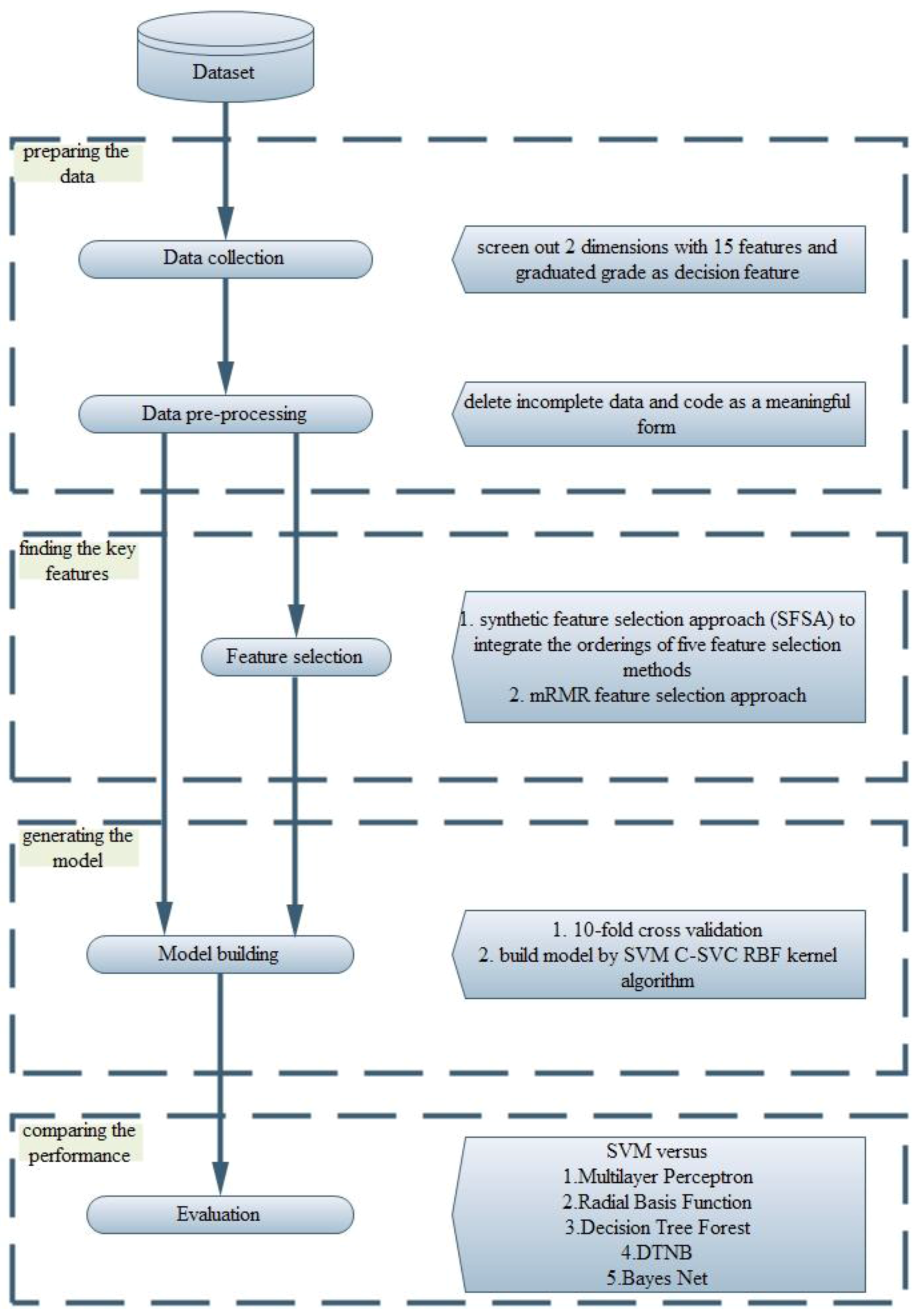
To facilitate understanding of the proposed method, the procedure of the proposed model is divided into five steps, which are illustrated in Figure 1 and introduced in detail as follows:

• Step 1. Data Collection

The research dataset was collected from an elementary school. This study was based on related literature, and 12 teachers were asked to participate in focus interviews. This study selected two dimensions with 15 features, and chose graduation grade as the decision feature (class) from the two databases, namely “Student Profile” and “Tutorship Record”. Next, the two types of data were combined into an integrated dataset. There were 883 records (students) in total, including two dimensions with 15 features and one decision feature, as shown in

Table 2. Description of collected dataset.

Dimension	Feature Name	Code	Value
Study Efficiency	Language average score	SE_1	Numeric, [0, 100]
	Math average score	SE_2	Numeric, [0, 100]
	Science average score	SE_3	Numeric, [0, 100]
	Arts average score	SE_4	Numeric, [0, 100]
	Social average score	SE_5	Numeric, [0, 100]
	Physical average score	SE_6	Numeric, [0, 100]
	Integrated activities average score	SE_7	Numeric, [0, 100]
	Behaviour average score	SE_8	Numeric, [0, 100]
Environment and Background	Education levels of parents	EB_1	Symbolic, [S, A, B, C, D]
	Occupations of parents	EB_2	Symbolic, [J0, J1, J2, J3, …, J9]
	Ages of parents	EB_3	Numeric, [30, …, 64]
	Number of children	EB_4	Symbolic, [C1, C2, …, C5]
	Self-ranking	EB_5	Symbolic, [S1, S2, S3, S4]
	Student Identity Background	EB_6	Symbolic, [G, ST, LST, S, T, F, FS, LS, L, AS, A, FT, FST]
	Teacher	EB_7	Symbolic, [T1, T2, …, T15]
Decision feature	The graduated grade of students	Class	Symbolic, [S, A, B]

Note: The meaning of the symbolic values will be explained in Section 4.1.

.

• Step 2. Data Pre-Processing

The integrated dataset has a total of 883 records. After some incomplete data are deleted, 870 records remain. Many records are in text format in the integrated dataset. In this step, they need to be coded in a meaningful form, such as symbolic or numeric values (see Table 2).

• Step 3. Feature Selection

This step introduces two different feature selection approaches.

a. Proposed Feature Selection Approach

First, five popular machine-learning methods are applied to select features: MLP, RBF, DA, CCN, and DTF. The five mentioned methods are often seen in related references and their common characteristics are as follows: (1) all belong to the supervised learning algorithm; and (2) all show the importance of features and have an ordering of features. Then, this step uses the proposed SFSA to determine the rankings of the five feature selection methods. SFSA is introduced as follows:

(1)

Apply the five feature selection methods to select features and rank the methods in terms of the importance of their selected features, where the first rank corresponds to a score of 1, the second corresponds to a score of 2, etc. If a feature is not selected by any feature selection method, then assign it a score of 16;

(2)

Sum the scores of the five feature selection methods for each feature; and

(3)

Rank the summed scores in ascending order: a larger score denotes a less important feature.

Second, based on the ranking of the proposed SFSA, we employ SVM to find the best feature set by sequentially removing the less important features.

b. mRMR Feature Selection Approach

mRMR [17] combines the maximal relevance criterion (Max-Relevance) and minimal redundancy (Min-Redundancy) condition and uses incremental search methods to optimise the maximal relevance criterion and minimal redundancy condition simultaneously, to find the near-optimal feature set. For comparison with the proposed SFSA, mRMR feature selection was used in this step. This paper used correlation-based feature selection (CFS) with a greedy stepwise search algorithm to guarantee the minimum redundancy between features and the maximum relevance of features and class labels, and then to find the key features of students’ academic achievement.

• Step 4. Model Building

The integrated dataset with 870 records was validated by 10-fold cross-validation. Based on the ranking of the proposed SFSA in Step 3, this step utilised an SVM (with the RBF kernel function) to find the best feature set by sequentially removing the less important features under accuracy criteria. The best feature set was obtained when the accuracy could no longer be improved. Then, this study built two models for students’ academic achievement: one uses all features to build the academic achievement appraisal model, and the other uses the best feature set to build the academic achievement appraisal model. For comparison, this step also uses the mRMR feature set and an SVM (with the RBF kernel function) to build an appraisal model.

• Step 5. Evaluation

This step utilised all features and the best feature set (selected from SFSA and mRMR) to build academic achievement appraisal models. Then, based on the three feature sets, the proposed model is compared with the listing methods in terms of accuracy; the listing methods include MLP, RBF, DTF, DTNB, and BN. Through an experiment, this paper will demonstrate that the proposed model has higher accuracy of classification. Moreover, the proposed model, based on finding the best feature set, is an effective method for predicting students’ academic achievement because it is a simpler model with fewer key features that can be applied to hybrid-type datasets.

4. Data Analysis and Results

This section verifies and compares the proposed model with the listing methods in terms of accuracy; the contents include the introduction of the collected dataset, verification and comparison, and finding and discussion.

4.1. Students’ Academic Achievement Dataset

The research dataset is collected from an elementary school in Central Taiwan, which was established in 1899. There are approximately 80 teachers and staff, and 40 classes from grade 1 to grade 6, with a total of 1300 students. In addition, this school is of medium scale and is the central school in a town in Central Taiwan. After the literature review and focus interviews were performed, 12 teachers were selected based on the collected databases “Student Profile” and “Tutorship Record” to discuss the related factors in students’ academic achievement. These twelve teachers gave consistent opinions. Two dimensions with 15 features were selected and the graduation grade was chosen as the decision feature (class). Next, this study concatenated the two kinds of databases into an integrated dataset with a total of 883 records (students), including two dimensions with 15 features and one decision feature. After the incomplete data were deleted, the research dataset contained 870 records, and many records were in the form of narrative text in the integrated dataset. Therefore, this study coded the records in a meaningful form (either symbol or numeric values).

The research dataset includes two dimensions with 15 features and one decision feature; all features are explained in the following.

4.1.1. Dimension of Study Efficiency

The dimension contains eight kinds of features as follows: language average score (SE_1), math average score (SE_2), science average score (SE_3), arts average score (SE_4), social average score (SE_5), physical average score (SE_6), integrated activities average score (SE_7), and behaviour average score (SE_8). Listed above are the average scores of students in various disciplines, and the eight features are presented as numeric values in Table 2.

4.1.2. Dimension of Environment and Background

There are seven kinds of features involved in this dimension as follows: education levels of parents (EB_1), occupations of parents (EB_2), ages of parents (EB_3), number of children (EB_4), self-ranking (EB_5), student identity background (EB_6), and teacher (EB_7). Some features are described by text records, which need to be coded in a meaningful form (symbolic or numeric values), as shown in Table 2. Next, the definitions of the seven features are described, and the way to code these features into meaningful symbols is explained as follows:

• Education levels of parents (EB_1): The level of education has an ordering; hence, this feature is coded in

  Table 3. The label of Education levels of parents (EB_1).

  Education Levels	Symbol
  Master’s degree or higher	S
  University or college	A
  Senior high school	B
  Junior high school	C
  Elementary school	D

  .
• Occupations of parents (EB_2): For this feature, the symbols of job classification can be obtained by using the information query system from the Council of Labour Affairs Vocational Training Council, Taiwan; this study lists the symbols in

  Table 4. The label of Occupations of parents (EB_2).

  Occupations Classification	Symbol
  Soldier (currently serving )	J0
  Administrative and Managers	J1
  Professionals	J2
  Technicians and associate professionals	J3
  Transactional staff	J4
  Service staff and sales staff	J5
  Agriculture, forestry, animal husbandry and fisheries staff	J6
  Skilled workers and technology-related personnel	J7
  Machinery and equipment operating workers and assembly workers	J8
  Unskilled workers and labour-type workers	J9

  .
• Ages of parents (EB_3): The feature is a numeric value, so there is no need to process it.
• Number of children (EB_4): This refers to the number of children in the student’s family. This feature is a numeric value, so there is no need to process it.
• Self-ranking (EB_5): This feature refers to the ranking of the student among his or her brothers and sisters. The feature is a numeric value, so there is no need to process it.
• Student identity background (EB_6): This refers to the student’s family situation, which is recorded as text in the school database. This study codes systematically each label of the feature in

  Table 5. The label of Student identity background (EB_6).

  Student Identity	Symbol
  Generally Student	G
  Aboriginal student	A
  Foreign child student	F
  Low-income household student	L
  Single-parent student	S
  Inter-generational education student	T

  . Furthermore, if a student has a variety of identities, the recorded markings will be joined. For instance, if the students’ identities are foreign student, low-income household student, and single-parent student, their record will contain “FLS”.
• Teacher (EB_7) refers to the tutor or teacher who has taught the student. Different teachers were coded from T1 to T15 based on the class taught.

4.1.3. Decision Class

Finally, the graduation grade is employed as the decision feature, which is the total score at graduation. It is coded as follows: scores greater than 90 are labelled as S, those in the range 80–89 are labelled as A, and those less than 70 are labelled as B.

4.2. Verification and Comparison

This section employs the integrated dataset as the research dataset to rank the features by using the proposed SFSA and then, based on the results, to sequentially remove the less important features for building the prediction model by an SVM. The proposed model is compared with the listing methods. After pre-processing, a total of 883 records were employed as the research dataset to evaluate the proposed model and compare it with the listing methods; part of the integrated dataset is shown in

Table 6. Partial integrated dataset.

SE_1	SE_2	SE_3	SE_4	SE_5	SE_6	SE_7	SE_8	EB_1	EB_2	EB_3	EB_4	EB_5	EB_6	EB_7	Class
83.78	80.55	79.50	87.25	77.23	81.63	89.25	83.45	B	J9	38.00	C3	S2	G	T1	A
88.80	75.50	78.98	87.50	80.25	87.60	88.50	84.88	B	J3	39.00	C3	S1	G	T1	A
78.10	79.83	75.23	84.88	70.85	82.78	88.50	87.70	B	J3	46.00	C4	S4	G	T1	A
…
73.83	61.83	73.80	79.50	74.40	79.78	86.00	85.25	B	J4	45.00	C1	S1	G	T15	B
93.25	80.43	88.70	91.00	88.58	89.13	92.38	91.50	C	J8	38.00	C3	S2	G	T15	S
89.00	78.68	80.65	89.88	83.25	86.98	91.88	92.25	A	J9	41.00	C2	S2	G	T15	A

Note: Class is the graduating grade.

. The class distribution of the integrated dataset is 299 in S grade, 479 in A grade, and 92 in B grade.

(A)

In feature selection: First, this study utilises MLP, RBF, DA, CCN, and DTF to rank the 15 features. Then, this study employs the proposed SFSA to synthesise the rankings of the five feature selection methods, as described in Step 3 in Section 3. The results of the SFSA are listed in

Table 7. Ranking score of all 15 features.

Feature	Ranking Score of Five Methods						Proposed Order
	MLP	RBF	DA	CCN	DTF	Summation
SE_1	3	1	1	2	1	8	1
SE_2	2	2	3	3	4	14	3
SE_3	1	3	2	1	2	9	2
SE_4	6	7	8	10	6	37	7
SE_5	4	8	7	8	3	30	4
SE_6	11	5	6	13	5	40	8
SE_7	10	4	16	16	8	54	11
SE_8	5	6	4	9	7	31	5
EB_1	8	15	12	11	13	59	12
EB_2	9	13	11	6	12	51	10
EB_3	14	9	16	14	10	63	15
EB_4	13	11	10	12	14	60	13
EB_5	16	14	9	7	15	61	14
EB_6	12	12	7	5	11	47	9
EB_7	7	10	5	4	9	35	6

. Second, the features selected using mRMR are ranked in the following order: SE_1, SE_2, SE_3, SE_4, SE_5, SE_6, SE_7, SE_8, EB_1, EB_2, EB_3, EB_4, EB_5, EB_6, and EB_7. The first three key features are language average score, math average score, and science average score for student’s academic achievement.

(B)

In building the model: The main objective is to build an optimal model with fewer features. First, this study uses all features to establish a prediction model. Second, the results of the proposed SFSA are utilised to sequentially remove the less important features for building the prediction model. Lastly, when removing features no longer improves the accuracy, the key features and optimal model have been obtained. The results of all features and selected features are shown in

Table 8. The result of sequentially deleting the least important feature (10-fold cross-validation).

Sequence	Excluded Feature	Remaining Features	Accuracy	Improvement
0	none	SE_1, SE_2, SE_3, SE_4, SE_5, SE_6, SE_7, SE_8, EB_1, EB_2, EB_3, EB_4, EB_5, EB_6, EB_7	83.57%	_
1	EB-3	SE_1, SE_2, SE_3, SE_4, SE_5, SE_6, SE_7, SE_8, EB_1, EB_2, EB_4, EB_5, EB_6, EB_7	81.15%	−2.42%
2	EB_5	SE_1, SE_2, SE_3, SE_4, SE_5, SE_6, SE_7, SE_8, EB_1, EB_2, EB_4, EB_6, EB_7	82.21%	−1.36%
3	EB_4	SE_1, SE_2, SE_3, SE_4, SE_5, SE_6, SE_7, SE_8, EB_1, EB_2, EB_6, EB_7	85.39%	1.82%
4	EB_1	SE_1, SE_2, SE_3, SE_4, SE_5, SE_6, SE_7, SE_8, EB_2, EB_6, EB_7	89.22%	5.65%
5	SE_7	SE_1, SE_2, SE_3, SE_4, SE_5, SE_6, SE_8, EB_2, EB_6, EB_7	85.83%	2.26%
6	EB_2	SE_1, SE_2, SE_3, SE_4, SE_5, SE_6, SE_8, EB_6, EB_7	92.23%	8.66%
7	EB_6	SE_1, SE_2, SE_3, SE_4, SE_5, SE_6, SE_8, EB_7	91.50%	7.93%
8	SE_6	SE_1, SE_2, SE_3, SE_4, SE_5, SE_8, EB_7	90.62%	7.05%

.

(C)

In the results: From Sequence 6 in Table 8, after six less influential features have been deleted, the accuracy is better than those of the full-feature model and other sequentially deleted feature models. Deleting the six least important features improved the accuracy by 8.66%. Therefore, the nine key features are from the categories “study efficiency” (SE_1, SE_2, SE_3, SE_4, SE_5, SE_6, and SE_8) and “environment and background” (EB_6 and EB_7), with the ordering: SE_1 > SE_3 > SE_2 > SE_5 > SE_8 > EB_7 > SE_4 > SE_6 > EB_6. Finally, this study uses the classifier with the six least important features deleted for comparison with other classifiers; the result is shown in

Table 9. The results of classification for 9 key features (10-fold cross-validation).

Algorithm	Proposed Feature Selection (FS)				mRMF FS
	Accuracy (SD)	Precision	Recall	F1	Accuracy (SD)	Precision	Recall	F1
MLP	86.94% (4.36)	0.89	0.89	0.89	84.82% (5.54)	0.84	0.91	0.87
RBF	87.18% (4.08)	0.86	0.92	0.89	83.63% (6.75)	0.82	0.92	0.87
DTF	89.64% (3.53)	0.90	0.92	0.91	88.70% (3.56)	0.89	0.91	0.90
DTNB	87.94% (3.65)	0.92	0.86	0.89	88.31% (3.46)	0.92	0.87	0.89
BN	87.57% (4.04)	0.92	0.86	0.89	88.84% (3.76)	0.93	0.87	0.90
SVM	92.23% (1.68)	0.94	0.92	0.93	90.05% (2.13)	0.91	0.91	0.91

. The proposed feature selection approach with SVM outperforms other classifiers in terms of accuracy, and the standard deviation is smaller than those of other classifiers. This paper also builds the appraisal model by using mRMR-selected features with an SVM; the results show that the proposed feature selection with an SVM outperforms mRMR-selected features with an SVM in terms of accuracy, as shown in Table 9.

4.3. Findings

Based on the previous case study and experimental results, the findings of this study are as follows:

(1)

Proposed feature selection approach: According to Table 8 and Table 9, the proposed feature selection approach can be effective in improving the classification accuracy, especially when the six least influential features have been deleted.

(2)

Key features: Based on Table 8, the nine key features that are related to students’ academic achievement are language, science, math, social science, behaviour, teacher, arts, physical education, and student identity background. The important results are described as follows:

(a)

No matter which method is used to select features, language, science, and math are important features; by all five feature selection methods, they are assigned the top three ranks. Therefore, it is clear that these results are in accordance with previous literature [61,62,63].

(b)

Furthermore, it is worth mentioning that the feature teacher (EB_7) also impacts students’ academic achievement [64,65,66,67].

(c)

Student behaviour in school, whether disciplined or not, affects academic achievement. The behaviour feature (SE_8) is related to the behaviour of elementary school students. A student who shows respect for his teacher and is polite and disciplined usually has high academic achievement [68,69,70].

(d)

Artistic ability is of great help for students in developing imagination and creativity, and it is very important to have confidence and creativity when facing challenges. Thus, if a student has higher artistic ability, he or she may have higher academic achievement [71,72].

(e)

The effect of physical education is similar to the effect of art ability for students; it can contribute to the academic achievement of students [73,74].

(f)

The student identity background (EB_6) feature is related to the student growth environment, which is an important factor that affects student academic achievement [75,76].

(3)

By repeatedly performing the experiment using different combinations of features, we found that SVM, which is used for classification in this study, can accurately identify the two least influential features: age of parents (SE_3) and self-rank (EB_5). The evidence shows that age of parents (SE_3) and self-rank (EB_5) are not important features for students’ academic achievement.

(4)

Two different kinds of feature selection approaches are used to select nine key features. The proposed method selects seven numeric and two symbolic features, while mRMR selects eight numeric and one symbolic feature. Then, the appraisal model is built by an SVM. The classification accuracy of the proposed feature selection approach is better than that of mRMR.

5. Conclusions

This study has proposed a hybrid model based on a SFSA for students’ academic achievement. The experimental results show that the performance of the proposed model is the best when the six least influential features are deleted. This study also compares the proposed feature selection approach and the mRMR feature selection approach, along with models obtained using other classifiers. Better accuracy is achieved by the proposed model with an SVM classifier when the six least influential features are deleted. Furthermore, this study finds the optimal model and the nine key features related to students’ academic achievement, which are ranked as follows: language, science, math, social science, behaviour, teacher, arts, physical education, and student identity background.

In future work, we will attempt to improve the accuracy of the model and increase its interpretation ability by using other classifiers and association rule analysis for feature selection. We can also utilise the following approach:

• Collect more samples for solving the class imbalance problem;
• Through stratified sampling, the class samples may be made more balanced; and
• Employ additional algorithms with different feature selection approaches.

References

- Fayyad, U.M.; Piatetsky-Shapiro, G.; Smyth, P.; Uthurusamy, R. Advances in Knowledge Discovery and Data Mining; AAAI Press: Palo Alto, CA, USA, 1996. [Google Scholar]
- Maimon, O.; Last, M. Knowledge Discovery and Data Mining: The Info-Fuzzy Network (ifn) Methodology; Springer Science & Business Media: Berlin, Germany, 2013; Volume 1. [Google Scholar]
- Smyth, P.; Pregibon, D.; Faloutsos, C. Data-driven evolution of data mining algorithms. Commun. ACM 2002, 45, 33–37. [Google Scholar] [CrossRef]
- Smyth, P. Breaking out of the Black-Box: Research Challenges in Data Mining. In Proceedings of the Sixth Workshop on Research Issues in Data Mining and Knowledge Discovery (DMKD2001), Santra Barbara, CA, USA, 20 May 2001. [Google Scholar]
- Gronlund, N.E. Assessment of Student Achievement; Allyn & Bacon Publishing: Needham Heights, MA, USA, 1998. [Google Scholar]
- Tionn, C.H. Zhang Dictionary of Psychology; Tung Hua Book Co., Ltd.: Taipei City, Taiwan, 2006. [Google Scholar]
- Blau, P.M.; Duncan, O.D. The American Occupational Structure; Free Press: New York, NY, USA, 1967. [Google Scholar]
- Coleman, J.S. Social capital in the creation of human capital. Am. J. Sociol. 1988, 94, S95–S120. [Google Scholar] [CrossRef]
- Meighan, R.; Bondi, H. Theory and Practice of Regressive Education; Educational Heretics Press: Shrewsbury, UK, 1993. [Google Scholar]
- Chen, K.X. Sociology of Education; National Taiwan Normal University Bookstore: Taipei City, Taiwan, 1993. [Google Scholar]
- Wang, W.K. Cognitive Development and Education: The Application of Piaget Theories; Wu-Nan Book Inc.: Taipei City, Taiwan, 1991. [Google Scholar]
- Chen, Y.H. The Research of Relationship Between Home Environment, Reading Motivation and Language Subject That Affects Elementary School Students Academic Achievement. Master’s Thesis, National Kaohsiung Normal University, Kaohsiung, Taiwan, 2001. [Google Scholar]
- Liao, R.Y. Analysis of High Academic Achievement Aboriginal Children and Family Factors-A Case Study of Community Balanao. Master’s Thesis, National Hualien Teachers College, Hualien, Taiwan, 2001. [Google Scholar]
- Hall, M.A. Correlation-Based Feature Selection for Machine Learning. Ph.D. Thesis, The University of Waikato, Hamilton, New Zealand, 1999. [Google Scholar]
- Bermingham, M.L.; Pong-Wong, R.; Spiliopoulou, A.; Hayward, C.; Rudan, I.; Campbell, H.; Wright, A.F.; Wilson, J.F.; Agakov, F.; Navarro, P.; et al. Application of high-dimensional feature selection: Evaluation for genomic prediction in man. Sci. Rep. 2015, 5. [Google Scholar] [CrossRef] [PubMed]
- Guyon, I.; Elisseeff, A. An introduction to variable and feature selection. J. Mach. Learn. Res. 2003, 3, 1157–1182. [Google Scholar]
- Peng, H.; Long, F.; Ding, C. Feature selection based on mutual information criteria of max-dependency, max-relevance, and min-redundancy. IEEE Trans. Pattern Anal. Mach. Intell. 2005, 27, 1226–1238. [Google Scholar] [CrossRef] [PubMed]
- Posner, M.I. Foundations of Cognitive Science; MIT Press: Cambridge, MA, USA, 1989. [Google Scholar]
- Rosenblatt, F. Perceptions and the Theory of Brain Mechanisms; Spartan Books: Washington, DC, USA, 1962. [Google Scholar]
- Bishop, C.M. Neural Networks for Pattern Recognition; Oxford University Press: Oxford, UK, 1995. [Google Scholar]
- Pal, S.K.; Mitra, S. Multilayer perceptron, fuzzy sets, and classification. IEEE Trans. Neural Netw. 1992, 3, 683–697. [Google Scholar] [CrossRef] [PubMed]
- Ruck, D.W.; Rogers, S.K.; Kabrisky, M.; Maybeck, P.S.; Oxley, M.E. Comparative analysis of backpropagation and the extended Kalman filter for training multilayer perceptrons. IEEE Trans. Pattern Anal. Mach. Intell. 1992, 14, 686–691. [Google Scholar] [CrossRef]
- Cybenko, G. Approximation by superpositions of a sigmoidal function. Math. Control Signals Syst. 1989, 2, 303–314. [Google Scholar] [CrossRef]
- Benvenuto, N.; Piazza, F. On the complex backpropagation algorithm. IEEE Trans. Signal Process. 1992, 40, 967–969. [Google Scholar] [CrossRef]
- Karlik, B.; Olgac, A.V. Performance analysis of various activation functions in generalized mlp architectures of neural networks. Int. J. Artif. Intell. Expert Syst. 2011, 1, 111–122. [Google Scholar]
- Broomhead, D.S.; Lowe, D. Multivariable functional interpolation and adaptive networks. Complex Syst. 1988, 2, 321–355. [Google Scholar]
- Billings, S.A.; Zheng, G.L. Radial basis function network configuration using genetic algorithms. Neural Netw. 1995, 8, 877–890. [Google Scholar] [CrossRef]
- Chen, S.; Cowan, C.F.N.; Grant, P.M. Orthogonal least squares learning algorithm for radial basis function networks. IEEE Trans. Neural Netw. 1991, 2, 302–309. [Google Scholar] [CrossRef] [PubMed]
- Rosenblum, M.; Yacoob, Y.; Davis, L.S. Human expression recognition from motion using a radial basis function network architecture. IEEE Trans. Neural Netw. 1996, 7, 1121–1138. [Google Scholar] [CrossRef] [PubMed]
- Friedman, J.H. Regularized Discriminant Analysis. J. Am. Stat. Assoc. 1989, 84, 165–175. [Google Scholar] [CrossRef]
- Klecka, W.R. Discriminant Analysis; Sage: Newcastle upon Tyne, UK, 1980. [Google Scholar]
- Loog, M.; Duin, R.P.W.; Haeb-Umbach, R. Multiclass linear dimension reduction by weighted pairwise fisher criteria. IEEE Trans. Pattern Anal. Mach. Intell. 2001, 23, 762–766. [Google Scholar] [CrossRef]
- McLachlan, G. Discriminant Analysis and Statistical Pattern Recognition; John Wiley & Sons: Chichester, UK, 2004; Volume 544. [Google Scholar]
- Bickel, P.J.; Levina, E. Some theory for Fisher’s linear discriminant function, ‘naive Bayes’, and some alternatives when there are many more variables than observations. Bernoulli 2004, 10, 989–1010. [Google Scholar] [CrossRef]
- Morrison, D.G. On the interpretation of discriminant analysis. J. Market. Res. 1969, 6, 156–163. [Google Scholar] [CrossRef]
- Fahlman, S.E.; Lebiere, C. The cascade-correlation learning architecture. In Advances in Neural Information Processing Systems 2 (NIPS 1989); Morgan Kaufmann Publishers Inc.: San Francisco, CA, USA, 1990. [Google Scholar]
- Fahlman, S.E. The Recurrent Cascade-Correlation Architecture; Carnegie-Mellon University, Department of Computer Science: Pittsburgh, PA, USA, 1991. [Google Scholar]
- Hwang, J.-N.; You, S.-S.; Lay, S.-R.; Jou, I.-C. The cascade-correlation learning: A projection pursuit learning perspective. IEEE Trans. Neural Netw. 1996, 7, 278–289. [Google Scholar] [CrossRef] [PubMed]
- Kovalishyn, V.V.; Tetko, I.V.; Luik, A.I.; Kholodovych, V.V.; Villa, A.E.P.; Livingstone, D.J. Neural Network Studies. 3. Variable Selection in the Cascade-Correlation Learning Architecture. J. Chem. Inf. Comput. Sci. 1998, 38, 651–659. [Google Scholar] [CrossRef]
- Hall, L.O.; Bensaid, A.M.; Clarke, L.P.; Velthuizen, R.P.; Silbiger, M.S.; Bezdek, J.C. A comparison of neural network and fuzzy clustering techniques in segmenting magnetic resonance images of the brain. IEEE Trans. Neural Netw. 1992, 3, 672–682. [Google Scholar] [CrossRef] [PubMed]
- Han, J.; Moraga, C. The Influence of the Sigmoid Function Parameters on the Speed of Backpropagation Learning. In IWANN ‘96, Proceedings of the International Workshop on Artificial Neural Networks: From Natural to Artificial Neural Computation; Springer: London, UK, 1995; pp. 195–201. [Google Scholar]
- Hoehfeld, M.; Fahlman, S.E. Learning with limited numerical precision using the cascade-correlation algorithm. IEEE Trans. Neural Netw. 1992, 3, 602–611. [Google Scholar] [CrossRef] [PubMed]
- Díaz-Uriarte, R.; de Andrés, S.A. Gene selection and classification of microarray data using random forest. BMC Bioinform. 2006, 7. [Google Scholar] [CrossRef] [PubMed]
- Cutler, L.B.a.A. Random forests. Mach. Learn. 2001, 45, 5–32. [Google Scholar]
- Ho, T.K. Random decision forests. In ICDAR ‘95, Proceedings of the Third International Conference on Document Analysis and Recognition, 14–15 August 1995; IEEE: Washington, DC, USA, 1995; pp. 278–282. [Google Scholar]
- Ho, T.K. The random subspace method for constructing decision forests. IEEE Trans. Pattern Anal. Mach. Intell. 1998, 20, 832–844. [Google Scholar]
- Vapnik, V. The Nature of Statistical Learning Theory; Springer Science & Business Media: Berlin, Germany, 2013. [Google Scholar]
- Vapnik, V.N.; Vapnik, V. Statistical Learning Theory; Wiley: New York, NY, USA, 1998; Volume 1. [Google Scholar]
- Cortes, C.; Vapnik, V. Support-vector networks. Mach. Learn. 1995, 20, 273–297. [Google Scholar] [CrossRef]
- Humby, E. Programs from Decision Tables; American Elsevier: New York, NY, USA, 1973. [Google Scholar]
- Kohavi, R. The power of decision tables. In Machine Learning: Ecml-95; Springer: Berlin, Germany, 1995; pp. 174–189. [Google Scholar]
- Hand, D.J.; Yu, K. Idiot’s bayes—Not so stupid after all? Int. Stat. Rev. 2001, 69, 385–398. [Google Scholar]
- Rish, I. An Empirical Study of the Naive Bayes Classifier. In Proceedings of the IJCAI 2001 Workshop on Empirical Methods in Artificial Intelligence, Seattle, WA, USA, 4 August 2001; IBM: New York, NY, USA, 2001; pp. 41–46. [Google Scholar]
- Ben-Gal, I. Bayesian networks. In Encyclopedia of Statistics in Quality and Reliability; John Wiley & Sons Ltd.: Chichester, UK, 2007. [Google Scholar]
- Jensen, F.V. An Introduction to Bayesian Networks; UCL Press: London, UK, 1996; Volume 210. [Google Scholar]
- Nielsen, T.D.; Jensen, F.V. Bayesian Networks and Decision Graphs; Springer Science & Business Media: Berlin, Germany, 2009. [Google Scholar]
- Hongeng, S.; Brémond, F.; Nevatia, R. Bayesian framework for video surveillance application. In Proceedings of the 2000 15th International Conference on Pattern Recognition, Barcelona, Spain, 3–7 September 2000; IEEE: New York, NY, USA, 2000; pp. 164–170. [Google Scholar]
- Lan, P.; Ji, Q.; Looney, C.G. Information fusion with bayesian networks for monitoring human fatigue. In Proceedings of the 2002 Fifth International Conference on Information Fusion, Annapolis, MD, USA, 8–11 July 2002; IEEE: New York, NY, USA, 2002; pp. 535–542. [Google Scholar]
- Sahin, F.; Bay, J. Learning from experience using a decision-theoretic intelligent agent in multi-agent systems. In Proceedings of the 2001 IEEE Mountain Workshop on Soft Computing in Industrial Applications, SMCia/01., Blacksburg, VA, USA, 27 June 2001; IEEE: New York, NY, USA, 2001; pp. 109–114. [Google Scholar]
- Fayyad, U.; Piatetsky-Shapiro, G.; Smyth, P. The kdd process for extracting useful knowledge from volumes of data. Commun. ACM 1996, 39, 27–34. [Google Scholar] [CrossRef]
- Barrow, L.H.; Kristo, J.V.; Andrew, B. Building bridges between science and reading. Read. Teach. 1984, 38, 188–192. [Google Scholar]
- Chall, J.S. Stages of Reading Development; McGraw-Hill: New York, NY, USA, 2011. [Google Scholar]
- Yore, L.D. A preliminary exploration of grade five students’ science achievement and ability to read science textbooks as a function of gender, reading vocabulary, and reading comprehension. In Proceedings of the 60th Annual Meeting of the National Association for Research in Science Teaching, Washington, DC, 23–25 April 1987. [Google Scholar]
- Friedman, I.A.; Kass, E. Teacher self-efficacy: A classroom-organization conceptualization. Teach. Teach. Educ. 2002, 18, 675–686. [Google Scholar] [CrossRef]
- Goddard, R.D. The impact of schools on teacher beliefs, influence, and student achievement. Teach. Beliefs Classr. Perform. Impact Teach. Educ. 2003, 6, 183–202. [Google Scholar]
- Goddard, R.D.; Hoy, W.K.; Hoy, A.W. Collective teacher efficacy: Its meaning, measure, and impact on student achievement. Am. Educ. Res. J. 2000, 37, 479–507. [Google Scholar] [CrossRef]
- Tschannen-Moran, M.; Barr, M. Fostering student learning: The relationship of collective teacher efficacy and student achievement. Leadersh. Policy Sch. 2004, 3, 189–209. [Google Scholar] [CrossRef]
- Bull, S.; Feldman, P.; Solity, J. Classroom Management: Principles to Practice; Routledge: Abingdon, UK, 2013. [Google Scholar]
- Burden, P.R. Classroom Management and Discipline: Methods to Facilitate Cooperation and Instruction; Longman Publishers USA: White Plains, NY, USA, 1995. [Google Scholar]
- Cangelosi, J.S. Classroom Management Strategies: Gaining and Maintaining Students’ Cooperation; John Wiley & Sons Incorporated: Chichester, UK, 2007. [Google Scholar]
- Barron, F.; Harrington, D.M. Creativity, intelligence, and personality. Ann. Rev. Psychol. 1981, 32, 439–476. [Google Scholar] [CrossRef]
- Smith, R.A.; Simpson, A. Aesthetics and Arts Education; University of Illinois Press: Champaign, IL, USA, 1991. [Google Scholar]
- Chomitz, V.R.; Slining, M.M.; McGowan, R.J.; Mitchell, S.E.; Dawson, G.F.; Hacker, K.A. Is there a relationship between physical fitness and academic achievement? Positive results from public school children in the northeastern united states. J. Sch. Health 2009, 79, 30–37. [Google Scholar] [CrossRef] [PubMed]
- Coe, D.P.; Pivarnik, J.M.; Womack, C.J.; Reeves, M.J.; Malina, R.M. Effect of physical education and activity levels on academic achievement in children. Med. Sci. Sports Exerc. 2006, 38, 1515–1519. [Google Scholar] [CrossRef] [PubMed]
- Astone, N.M.; McLanahan, S.S. Family structure, parental practices and high school completion. Am. Sociol. Rev. 1991, 56, 309–320. [Google Scholar] [CrossRef]
- Nisbet, J. Family environment and intelligence. Eugen. Rev. 1953, 45, 31–40. [Google Scholar] [PubMed]
Figure 1.
The procedure of proposed method (revised from [60]).