Optimized Charging Scheduling with Single Mobile Charger for Wireless Rechargeable Sensor Networks

1
School of Medical Information Engineering, Jining Medical University, Rizhao 276826, China
2
College of Computer, Nanjing University of Posts and Telecommunications, Nanjing 210003, China
*
Author to whom correspondence should be addressed.
Symmetry 2017, 9(11), 285; https://doi.org/10.3390/sym9110285
Submission received: 7 October 2017
/
Revised: 15 November 2017
/
Accepted: 16 November 2017
/
Published: 21 November 2017
Abstract
:Due to the rapid development of wireless charging technology, the recharging issue in wireless rechargeable sensor network (WRSN) has been a popular research problem in the past few years. The weakness of previous work is that charging route planning is not reasonable. In this work, a dynamic optimal scheduling scheme aiming to maximize the vacation time ratio of a single mobile changer for WRSN is proposed. In the proposed scheme, the wireless sensor network is divided into several sub-networks according to the initial topology of deployed sensor networks. After comprehensive analysis of energy states, working state and constraints for different sensor nodes in WRSN, we transform the optimized charging path problem of the whole network into the local optimization problem of the sub networks. The optimized charging path with respect to dynamic network topology in each sub-network is obtained by solving an optimization problem, and the lifetime of the deployed wireless sensor network can be prolonged. Simulation results show that the proposed scheme has good and reliable performance for a small wireless rechargeable sensor network.
1. Introduction
Wireless sensor network (WSN) is a novel technology for acquiring information and processing information, and it can be widely used in environmental detection, civil infrastructure, target tracking, information security, intelligent medical care, etc. Since sensor nodes in WSN are usually powered by rechargeable batteries, which have been constrained energy capacity and limited lifetime of network, many researchers have devoted efforts to developing effective algorithms on WSN to alleviate this problem [1,2,3,4]. To deal with this problem, reducing energy consumption has become the main focus in wireless sensor networks in the past decade. Since it is infeasible or risky to replace a sensor’s battery in some special deployment environment [5], most of the research literatures aim to maximize the lifetime of network. Although their proposed methods can prolong the lifetime of a network to some extent, the energy of sensor nodes would eventually run out and the deployed network stop working.
A recent breakthrough in wireless power transfer technique [6] provides a new choice for solving the energy-constrained problem, which can make it promising to recharge energy for prolonging the lifetime of network. The main objective of this paper is to address how to use wireless recharging in a traditional battery powered wireless sensor network. Here we call such a network a wireless rechargeable sensor network (WRSN). Wireless charging technology is usually used to charge sensor nodes to supplement energy in WRSN. When wireless charging technology is applied to the mobile charger, the mobile charger can be scheduled to recharge sensor nodes in WRSN. Xie et al. [7] studied an optimization problem for recharge schedule and joint routing. They also showed a proof that the optimal traveling path is the shortest Hamiltonian cycle. In [8,9,10], a novel method is proposed to schedule a mobile charger to visit fixed locations. The sensor nodes were recharged if the locations of the sensor nodes were in the charging range of the mobile charger. This method has a high requirement for mobile chargers. In [11], Wang et al. proposed a new strategy to recharge sensor nodes with the minimum total visiting cost of the mobile chargers. A new algorithm which can be considered as the traveling salesman problem based on the energy consumption of sensor nodes is proposed to minimize distance in [12,13]. In [14], mobile chargers recharge sensor nodes and collect data to go through the sensor nodes following a fixed path at the same time. Their method can prolong the lifetime of sensor nodes, but it is difficult to apply in practice.
In WRSNs, mobile changers are expensive equipment. If a single mobile charger is sufficient to complete requested charging tasks, in general, we may not increase the number of mobile chargers to improve the quality of service. Therefore, a single mobile changer scheme has been used in smaller scale sensor networks. The single mobile changer scheme has low cost and the charging plan is relatively simple. However, due to the limited charge capacity of the single mobile changer, charging time and visiting path require a reasonable design and planning. The multiple mobile chargers scheme can be used to process tasks in a parallel manner for WRSN and this scheme can reduce the charging delay. It is mainly applied to larger scale sensor networks. The scalability of the charging planning is good, but the total costs of the multiple mobile charger scheme are higher.
According to the number of deployed mobile chargers, the existing work can be grouped into two categories: single mobile charger scheme [9,15,16,17] and multiple mobile chargers [10,18,19,20]. In [17], the authors proposed a hybrid clustering charging algorithm (HCCA). A means algorithm was used to compute energy core set in order to reduce large recharging times and long traveling time. With the rapid development of wireless charging technology, a sensor node is recharged while it is only in the limited charging ranges of mobile chargers [21]. In practical application, it is inefficient to charge multiple sensor nodes with a mobile charger at the same time. Moreover, since mobile chargers are often costly, they have to be used as little as possible.
Although previous methods can prolong the lifetime of WRSN, the following problems need to be paid more attention and discussed thoroughly.
- (1)
- The effect of the moving speed of the mobile charger:
- (2)
- Previous work failed to neglect the importance of the location of service station:
- (3)
- Non periodic charging problem in WRSN:
- (4)
- How to apply the rest sensor nodes if the residual energy of a part of nodes in the network reaches the threshold.
In this work, we combine the mobile charger and the wireless energy transfer together to provide a dynamic scheduling strategy for mobile charger based on the optimization problem. In order to achieve this goal and fully improve the utilization rate of mobile charger, the single charger scheme is adopted to recharge sensor nodes. To solve the optimization problem, a novel recharging scheduling is proposed to maximize the vacation time of mobile charger. This method can give a reasonable visiting path through the local optimum of the sub-networks. As a result, the proposed scheme can prolong the lifetime of a network significantly.
Different from the existing single mobile charger schemes, the contributions of this work are summarized briefly as following:
- (1)
- We propose a new method to determine the optimal location for the service station.
- (2)
- The WRSN is divided into several sub networks. In the premise of ensuring certain coverage, not all sensor nodes in each sub network are selected for the active nodes. When the residual energy of the sensor node for the active nodes is lower than the threshold value, the sensor node stops working and waits for charging.
In order to improve the network lifetime and to consider the network service quality, in this work, a novel and optimal charging scheduling algorithm which can maximize the vacation time of the mobile charger is proposed.
2. Related Models and Problem Statement
2.1. Network and Charging Model
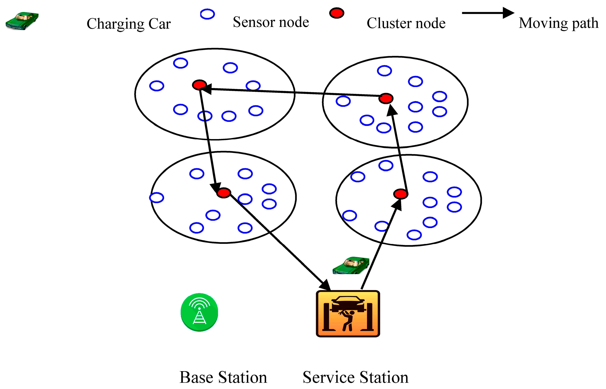
In this section, the network architecture for WRSN is introduced. As shown in Figure 1, a WRSN is made up of five components: base station, mobile charger, sensor node, cluster node and service station, which are categorized as follows.
Base station: The base station is used for collecting sensing data and performing management of the network. The mobile charger can be commanded remotely by the user of the network via the base station. It also has computing capabilities to perform the tasks of calculating recharge sequences. The symbol represents the base station.
Mobile charger: It is responsible for providing the energy supply for the rechargeable sensors. A mobile charger denoted by has a positioning system and knows its location. The locations of sensor nodes are known to the mobile charger and base station. The mobile charger is equipped with high density battery packs and charging coils. It can communicate with the base station via long distance communication technologies.
Sensor node: The sensor node collects data from the monitoring region, and sends the collection data to its cluster node. It reports its battery status to the cluster node. When the energy of the sensor node drops to the threshold value, the sensor node is waiting for the mobile charger to charge.
Cluster node: A cluster node is a sensor node denoted by symbol that collects the status information of sensor nodes in the sub network. Each cluster node is responsible for a number of nearby sensor nodes. In a circular fashion, a cluster node is selected at random so that the energy consumption load of the whole network is distributed to each sensor node. This approach improves the lifetime of the entire network.
Service station: When a mobile charger almost depletes its own energy or completes recharging nodes, it returns to the service station for energy supply or maintenance. The symbol represents service station. Due to the maintenance and energy supplement of mobile charger in service station, the location of the service station has certain significance.
In a WRSN, sensor nodes are deployed in a sensing field and they are no longer moving. Let represent the topology of the sensor nodes. denotes the set of sensor nodes, and is the set of edges with the distance between two sensor nodes. In WRSN, each sensor can transmit data to other sensors within its transmission range by single hop or multi-hop. In addition, every sensor can be recharged by a mobile charger. The time for recharging sensor by mobile charger is denoted by . Assume that the charging route to WSN for a mobile charger is . That is to say, mobile charger starts from service station. It visits all sensor nodes in sequence , and finally moves back to the service station.
The sensor nodes in WSN can be divided into three parts, in detail these are: active sensor node, sleep sensor node and inactive sensor node. The active sensor node which can collect information is a working node. Sleep sensor node represents an energy depleted node and waits for recharging. Inactive sensor node is not working, but it’s full of energy. Every sensor node has a battery capacity of , and needs a minimum energy to work properly. The time of visit all the sensor nodes for the mobile charger is denoted by symbol . The total time has three parts. Travel time for the mobile charger is expressed as . Charging time for the remaining energy of sensor nodes to reach the threshold (these nodes are called sleep nodes) is denoted by . Charging time for a node in a working state is denoted by symbol . The total distance of the movement path is the distance from , through to . The total distance can be expressed in the following expression,
where is the distance between sensor node and . In particular, denotes the distance between service station and the first be charged node. is the distance between service station and the last node to have been charged. Assume that mobile charger moves at a constant speed , can be calculated as the following expression.
Assume that the all sensor nodes have the same energy, and the initial energy of each node is full. The charging time of the mobile charger for active node is related to their remaining energy. With the energy consumption of collecting and sending data, the active nodes achieve the minimum value and wait for charging. Inactive sensor nodes do not need to be charged. At a certain time, the set of active nodes is represented as , and the set of sleep sensor nodes is represented as . The set of inactive sensor nodes is denoted by .
The charging time of the sleep node and the active node are respectively expressed as:
where denotes the charging rate of charger, and it is constant and uniform for all sensor nodes. The residual energy of active sensor node denoted by should satisfy .
To design a reasonable scheduling strategy for wireless sensor network, the total time to traverse all sensor nodes for mobile charger can be calculated as:
2.2. The Model of Energy Consumption
If the energy consumption of the sensor nodes is not balanced, the energy of some sensor nodes is likely to be exhausted. In practical application, each node transmits data to a selected node which is called the cluster node and places a heavy burden on the relay data. Some sensor nodes may be compelled to go to sleep because energy is depleted.
To balance the network load and prolong the network lifetime, according to the initial network deployment, the network is divided into several clusters, and each cluster can be seen as a sub network. In [22], the cluster node is responsible for sending the collection information in multi hop or single hop to the base station. The initial energy of each sensor node is denoted as . In this paper, the initial energy is fully charged. That is to say, is equal to . When the energy of the sensor node is lower than the threshold value , sensor node stops working and waits for recharging.
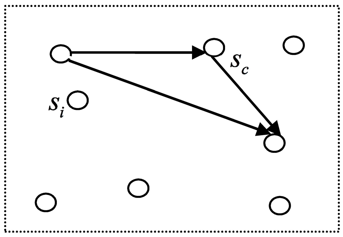
The largest energy consumption for sensor node is transmission data, and energy consumption of data transmission is growing rapidly with the increase of the distance. The means of transmitting data in the cluster is shown in Figure 2. Data information can be sent from one node to another node by single hop or relay node. In order to reduce the energy consumption, an optimal path should be selected to transmit data. The energy consumption is calculated as follows:
- (1)
- When , the formula for energy consumption is expressed as the following equation.
- (2)
- When , the formula for energy consumption is expressed as the following equation.where is a determined value, while and are the attribute parameters of sensor node, and is energy consumption of one sensor node receiving or transmitting 1 bit data. The symbol represents the amount of data that can be sent. Its unit is bit. The symbol is a Boolean variable. When the two nodes transfer data by single hop, the value of is zero; Otherwise, the value of is 1. Symbol represents the distance between the communication nodes.
2.3. Problem Formulation
Give a wireless sensor network with nodes and parameters , and , the distance between any pair of nodes, find a charging path starting from service station and visit each sensor node exactly only once to charge them. In order to achieve this goal, novel scheduling algorithm is designed to maximize the time ratio of the mobile charger at the service station.
At the same time, this method should guarantee normal operation in each sub network. In order to find optimal path, we can obtain the following optimization objective function from the above analysis.
After finishing recharging for wireless sensor node, mobile charger returns back to the service station to be serviced and gets ready for the next charging trip. The time for the mobile charger staying at the service station is called vacation time denoted by The symbol represents the Equation (5). It is very difficult to solve the above optimization function. In this paper, the network is divided into several sub networks.
3. Charging Scheduling Policy
3.1. Location Problem of Service Station
In this subsection, we determine the location of the service station in WSN. When the sensor nodes are deployed, in order to provide better network service quality, we should determine the location of the service station. The location of the service station is regarded as the single point optimal location problem. When there are a large number of sensor nodes in WSN, in this paper, the network is divided into several sub networks according to the distance between sensor nodes. Each sub network is a cluster. Firstly, a center node such that the maximum distance to each node is minimized in each cluster is determined, and then the optimal location of the service station is determined according to the location of the center node. Variable is introduced in the following equation. The method of center node in each sub network is determined as follows.
The mathematical model of determining the center node can be expressed as Equation (9),
where is the shortest distance between sensor node and sensor node . In this paper, the Floyd algorithm [23] is used to obtain the shortest distance. The optimization objective function [9] is a 0–1 integer programming problem, and we can use the following steps to calculate the center node and the center radius in each sub network .
- (1)
- Compute the shortest distance in each sub network using Floyd algorithm.
- (2)
- Calculate the distance between each sensor node and its farthest sensor node . can be expressed as .
- (3)
- Find the minimum , that is to say, .
After the above steps, we can obtain center node and center radius in each sub network. Assume that the coordinate position of the service station is . The coordinate positions of center node are denoted by . Location of service station can be obtained through the following optimization objective function.
3.2. The Selection of Active Nodes
In this section, we consider the coverage of the sub network. In order to make full use of the network resources, optimize the energy consumption and prolong the network life time, sensor nodes are selected to become the current active nodes. They can guarantee a certain coverage rate . Symbol denotes the -th sub network. When the energy consumption of the active node drops to a threshold value , or the energy consumption of the active node achieve maximum value , the state of the sensor node becomes a sleep node. An active node should be selected from other qualified nodes. The number in different sub network may be different. A set of sensor nodes in a sub network can be denoted as . Active sensor nodes are selected using the following calculation method.
denotes the residual energy of sensor node , while denotes the coverage area of sensor node . Center radius of the center node is denoted by , and denotes the overlapping coverage area of active nodes. Energy consumption of sensor node is denoted by in -th active period. We assume that all sensor nodes are homogeneous and the sensing radius of the sensor node is . It is assumed that all sensor nodes have the same sensing radius. We can compute as follows.
3.3. Optimal Path Selection
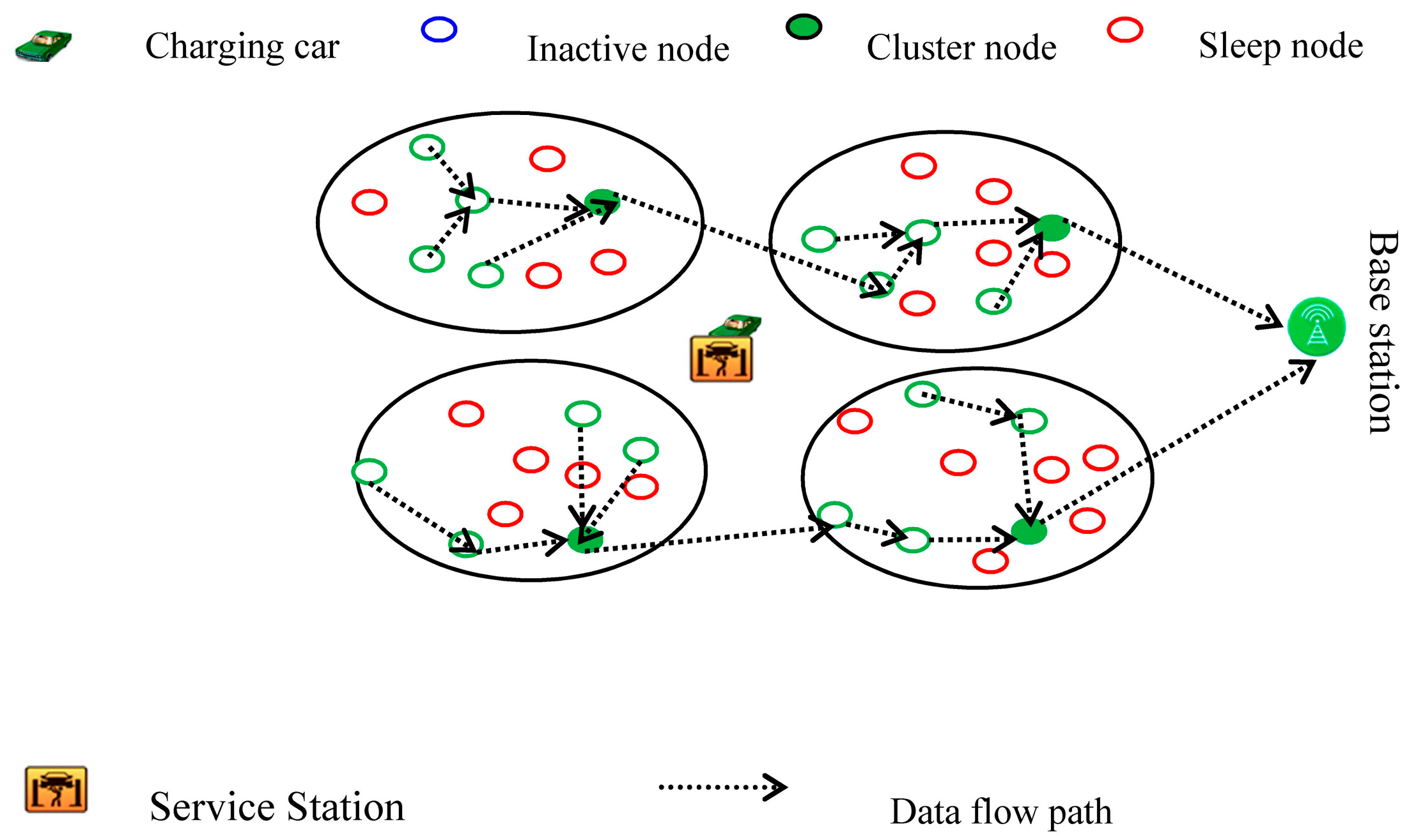
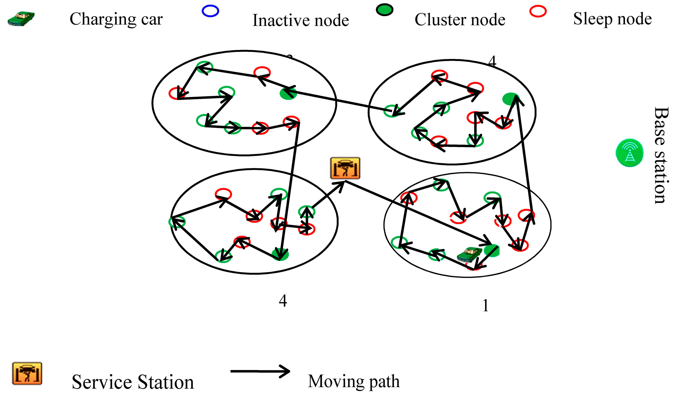
Each sensor node reports its current battery status and remaining battery energy to the cluster node which will send the collected energy status information to the base station. According to the energy state of the node, the base station schedules the charging route of mobile charger. In this paper, it is assumed that the positions of sensor nodes are no longer moving after the sensor nodes are deployed. In WSN, the division of the sub network is fixed, but the topology of the active node in each sub network is dynamic. As shown from Figure 3 and Figure 4, the network topology is different in different time periods.
When sensor nodes are deployed, the energy of each sensor node is full. A period of the network has two phases: charging time of mobile charger and vacation time of mobile charger. Because of dynamic change of the transmission data quantity and the topology structure in each sub network, the charging time of the traversing node is not always the same.
In any case, the charging sequence of the sensor nodes must satisfy certain conditions. Before being charged, the energy and the number of active sensor nodes in each sub network are sufficient to maintain the normal work, that is, the residual energy of the sensor nodes is not less than .
Generally speaking, starting from the service station, the mobile charger traverses all sensor nodes in WSN, and finally comes back to the service station. The optimization objective function (8) can be described as the following: traverse all sensor nodes in the wireless sensor network, seeking the shortest Hamilton path. The problem of Hamilton path is an NP hard problem. In all paths (the number of the paths is ), to find one optimal path, the computation complexity is high, and the calculation cannot even be completed. In this paper, the constraint conditions of optimal path are relaxed, and the global optimal is transformed into local optimal. The combination of the optimization routes in each sub network is the charging path of the mobile charger.
The base station analyzes and calculates the state of sensor nodes and the residual energy of sensor nodes, and then sorts the charging priority of the sub network based on the results of this analysis and calculations. When a sub network is charged, we must ensure that other sub networks can work properly. If the mobile charger leaves the service station too early, the utilization rate of the mobile charger will come down. If the time of leaving the service station for the mobile charger is too late, the sub network will not work properly because the energy of many nodes has been depleted. It is difficult to estimate the energy consumption of one sensor node for some time in the future. To facilitate the discussion, when the mobile charger begins to recharge the sensor node, the energy consumption rate of the active nodes for the other sub networks is the same. The energy consumption rate is denoted by . In fact, the energy consumption of the cluster node is larger than the general sensor node. When the mobile charger is in vacation status, the energy consumption of the sensor node is calculated according to the actual situation.
In this sub section, we mainly focus on the charging path of the mobile charger in a wireless sensor network. The base station should control the time of the mobile charger starting from the service station. is the distance between service station and active nodes which need to be recharged in sub network , and the time of mobile charger to the first charging node is expressed as Equation (13).
when the mobile charger reaches the most need to be charged active node, the remaining energy of active node is not less than . Mathematically, to charge the first sub network, the following conditions should be satisfied.
The symbol denotes the minimum residual energy of active nodes in the first sub network.
When the mobile charger completes the charging of all sensor nodes in sub network , the distance between the last node to be charged in the sub network and the first node to be charged in the sub network should be computed. Accordingly, we can obtain the following expressions.
The same method can be used to obtain the relationship and conditions when the mobile charger recharges the sensor nodes of the other sub network. Combining Equations (13)–(15), the optimization objective function (8) can be re-expressed as:
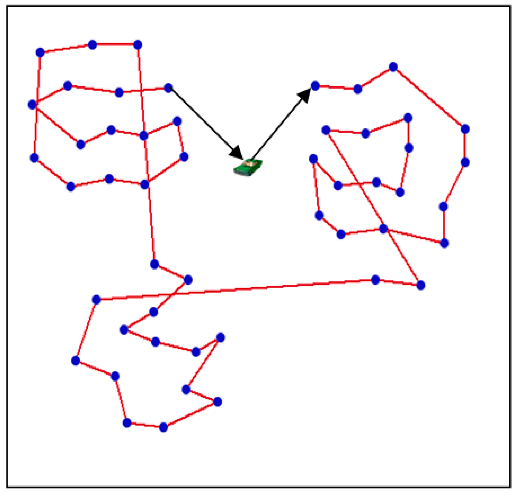
The constraint conditions of the above optimization objective function are similar, but the constraint condition is mutually restricted, and it has the characteristics of a recursive function. The charging route in a certain period is shown in Figure 5.
The whole algorithm can be described as follows:
- (1)
- Use the principle of proximity to determine the division of sub networks;
- (2)
- Determine the position of the mobile charger;
- (3)
- Determine the active nodes and select cluster nodes in each sub network;
- (4)
- Update the active nodes according to the energy consumption of the node, and update the cluster nodes correspondingly;
- (5)
- According to the energy consumption of each sensor node in the sub network and the overall energy consumption in each sub network, the recharging scheduling strategy is determined. In each sub network, the residual energy of the last active nodes is no less than before being charged. It can make full use of the energy of each node;
- (6)
- After finishing the charging nodes, the mobile charger returns to the service station and waits for the next charge.
4. Simulation Results
In this section, examples of our proposed scheme are given in different sensor nodes. Figure 6, Figure 7 and Figure 8 show the travelling paths with different sensor nodes. Assume that sensor nodes are deployed in a 100 m × 100 m square area. In the square area, there is one base station and one service station which can accommodate the mobile charger. The Experimental simulations are achieved in Matlab R2008. The sensor nodes meet the following conditions:
- (1)
- The sensor nodes are fixed.
- (2)
- The sensor nodes send data through single hop or multiple hops.
- (3)
- The sensor nodes know their locations with the help of GPS.
- (4)
- Euclidean distance can be obtained by mobile charger with the help of GPS and location algorithm.
We know the location information of sensor nodes, base stations by positioning technology in advance. The location of service station can be calculated. According to the charging scheduling policy in Section 3, we simulate the charging planning route of the mobile charger for the senor nodes. Figure 6, Figure 7 and Figure 8 show the optimal travelling path in a different number of sensor nodes.
In Figure 6, the total travelling distance of the mobile charger for 30 sensor nodes is or so 654 m. In Figure 7, the total travelling distance of the mobile charger for 40 sensor nodes is about 789 m. In Figure 8, the total travelling distance of the mobile charger for 50 sensor nodes is about 1093 m.
Under the same condition, the average recharging time for 30 sensor nodes is about 6327 s, while the average recharging time for 40 sensor nodes is about 8394.5 s, and the time for recharging 50 sensor nodes takes 10,546.5 s approximately. Ratios of vacation time for the mobile charger are 47.28%, 30.05 and 12.11%, respectively. The utilization rate of a single mobile charger is very high for a relatively small network. In a large-scale network, for an increase in the number of sensor nodes, charging time and travelling distance are gradually increasing, so the single mobile charger scheme is not suitable for a large wireless rechargeable sensor network.
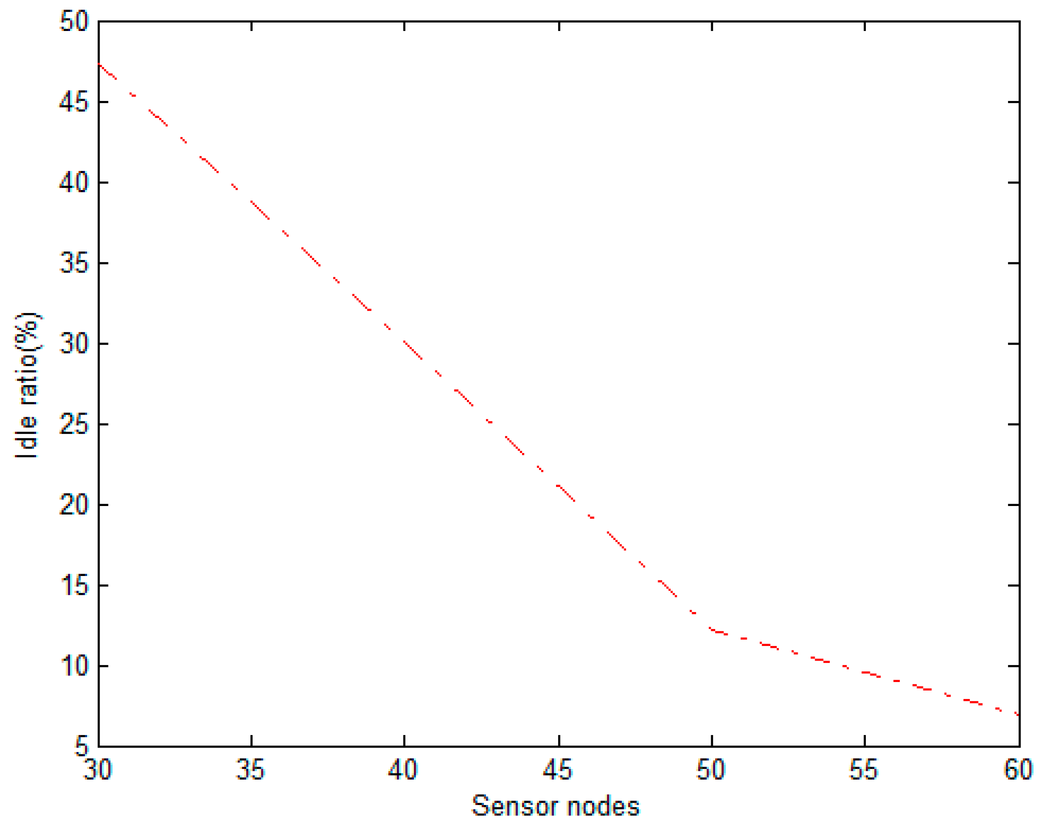
In order to express the advantages of our scheme, we compare the performance of our proposed scheme with the literature [17]. Compared to [17], we can see that our scheme has a small travelling path when the scale of sensor nodes is small from Figure 9. As the scale of sensor nodes increases, the travelling path of HCCA is better than ours. Our scheme is more suitable for small WSNs. As shown from Figure 10, we see that the recharging time of our scheme is low compared to that of the scheme in literature [17]. The change in idle rate is given in Figure 11. When the number of nodes is 60, the utilization of charging equipment can achieve about 95%.
5. Conclusions
In this section, the conclusion and future work are summarized. In this work, we have studied the optimization recharging path problem for a wireless sensor network. In order to obtain the reasonable charging route for sensor nodes, we formulate the problem, and transform the global optimization problem into a local optimization problem. Our charging scheduling strategy can ensure the normal work of the wireless sensor network under certain constraint conditions. Meanwhile, it can maximize the vacation ratio of single mobile charger. Simulation results show that our optimal scheduling algorithm can complete the recharging task well for a small wireless sensor network.
In future work, we will try to design a charging scheduling algorithm for a large-scale sensor network in multiple mobile chargers. Moreover, we will try to find the minimum number of mobile chargers for recharging a large-scale sensor network.
Acknowledgments
The work is supported by research support fund for teachers in Jining Medical University (No. JY2017KJ053).
Author Contributions
Qihua Wang and Fanzhi Kong proposed the methodology. Qihua Wang wrote the paper. Meng Wang and Huaqun Wang performed the experiments of this methodology.
Conflicts of Interest
The authors declare no conflict of Interest.
References
- Lin, C.; Wu, G.; Xia, F.; Li, M.; Yao, L.; Pei, Z. Energy efficient ant colony algorithms for data aggregation in wireless sensor networks. J. Comput. Syst. Sci. 2012, 78, 1686–1702. [Google Scholar] [CrossRef]
- González-Potes, A.; Mata-López, W.A.; Ochoa-Brust, A.M.; Escobar-del Pozo, C. Smart Control of Multiple Evaporator Systems with Wireless Sensor and Actuator Networks. Energies 2016, 9, 142. [Google Scholar] [CrossRef]
- Amaldi, E.; Capone, M. Design of wireless sensor networks for mobile target detection. IEEE/ACM Trans. Netw. 2012, 20, 784–797. [Google Scholar] [CrossRef]
- Dervis, K.; Selcuk, O. Cluster based wireless sensor network routing using artificial bee colony algorithm. Wirel. Netw. 2012, 18, 847–860. [Google Scholar]
- Geoffrey, W.A. Deploying a wireless sensor network on an active volcano. IEEE Internet Comput. 2006, 10, 18–25. [Google Scholar]
- Kurs, A.; Karalis, A.; Robert, M.; Joannopoulos, J.D.; Fisher, P.; Soljacic, M. Wireless power transfer via strongly coupled magnetic resonances. Science 2007, 317, 83–86. [Google Scholar] [CrossRef] [PubMed]
- Xie, L.; Shi, Y.; Hou, Y.T.; Sherali, H.D. Making sensor networks immortal: An energy-renewal approach with wireless power transfer. IEEE/ACM Trans. Netw. 2012, 20, 1748–1761. [Google Scholar] [CrossRef]
- Wang, C.; Yang, Y.; Li, J. Stochastic mobile energy replenishment and adaptive sensor activation for perpetual wireless rechargeable sensor networks. In Proceedings of the IEEE Wireless Communications and Networking Conference (WCNC), Shanghai, China, 7–10 April 2013; pp. 974–979. [Google Scholar]
- Guo, S.T.; Wang, C.; Yang, Y.Y. Joint mobile data gathering and energy provisioning in wireless rechargeable sensor networks. IEEE Trans. Mob. Comput. 2014, 12, 2836–2852. [Google Scholar] [CrossRef]
- Liu, B.H.; Nguyen, N.T.; Pham, V.T.; Lin, Y.X. Novel methods for energy charging and data collection in wireless rechargeable sensor networks. Int. J. Commun. Syst. 2015, 30, e3050. [Google Scholar] [CrossRef]
- Wang, C.; Li, J.; Ye, F.; Yang, Y. Multi-vehicle coordination for wireless energy replenishment in sensor networks. In Proceedings of the 2013 IEEE 27th International Symposium on I Parallel & Distributed Processing (IPDPS), Boston, MA, USA, 20–24 May 2013; pp. 1101–1111. [Google Scholar]
- He, L.; Fu, L.; Zheng, L.; Gu, Y.; Cheng, P.; Chen, J.; Pan, J. ESync: An energy synchronized charging protocol for rechargeable wireless sensor networks. In Proceedings of the 15th ACM International Symposium on Mobile Ad Hoc Networking and Computing, Philadelphia, PA, USA, 11–14 August 2014; pp. 247–256. [Google Scholar]
- Guo, S.T.; Wang, C.; Yang, Y.Y. Mobile data gathering with wireless energy replenishment in rechargeable sensor networks. In Proceedings of the IEEE Conference on Computer Communications (INFOCOM), Turin, Italy, 14–19 April 2013; pp. 1932–1940. [Google Scholar]
- Li, J.; Zhao, M.; Yang, Y. OWER-MDG: A novel energy replenishment and data gathering mechanism in wireless rechargeable sensor networks. In Proceedings of the IEEE Global Communications Conference (GLOBECOM), Anaheim, CA, USA, 3–7 December 2012; pp. 5350–5355. [Google Scholar]
- Zhao, M.; Li, J.; Yang, Y. A framework of joint mobile energy replenishment and data gathering in wireless rechargeable sensor networks. IEEE Trans. Mob. Comput. 2014, 12, 2689–2705. [Google Scholar] [CrossRef]
- Angelopoulos, C.M.; Nikoletseas, S.E.; Raptis, T.P. Wireless energy transfer in sensor networks with adaptive limited knowledge protocols. Comput. Netw. 2014, 70, 113–141. [Google Scholar] [CrossRef]
- Lin, C.; Wu, G.W.; Obaidat, M.S.; Yu, C.W. Clustering and splitting charging algorithms for large scaled wireless rechargeable sensor networks. J. Syst. Softw. 2016, 113, 381–394. [Google Scholar] [CrossRef]
- Madhja, A.; Nikoletseas, S.; Raptis, T.P. Distributed wireless power transfer in sensor networks with multiple mobile chargers. Comput. Netw. 2015, 80, 89–108. [Google Scholar] [CrossRef]
- Dai, H.; Wu, X.; Chen, G.; Xu, L.; Lin, S. Minimizing the number of mobile chargers for large-scale wireless recharge able sensor networks. Comput. Commun. 2014, 46, 54–65. [Google Scholar] [CrossRef]
- Madhja, A.; Nikoletseas, S.; Raptis, T.P. Hierarchical, collaborative wireless energy transfer in sensor networks with multiple Mobile Chargers. Comput. Netw. 2016, 97, 98–112. [Google Scholar] [CrossRef]
- Cheng, P.; He, S.; Jiang, F.; Gu, Y.; Chen, J. Optimal scheduling for quality of monitoring in wireless rechargeable sensor networks. IEEE Trans. Wirel. Commun. 2013, 12, 3072–3084. [Google Scholar] [CrossRef]
- Heinzelman, W.B.; Chandrakasen, A.P.; Balakrishnan, H. Application-specific protocol architecture for wireless micro sensor networks. IEEE Trans. Wirel. Commun. 2002, 4, 660–670. [Google Scholar] [CrossRef]
- Floyd, R.W. Algorithm 97: Shortest path. Commun. ACM 1962, 6, 345. [Google Scholar] [CrossRef]
Figure 1.
The network architecture for a wireless rechargeable sensor network (WRSN).

Figure 2.
Data multi-hop transmission.

Figure 3.
Network topology in time .
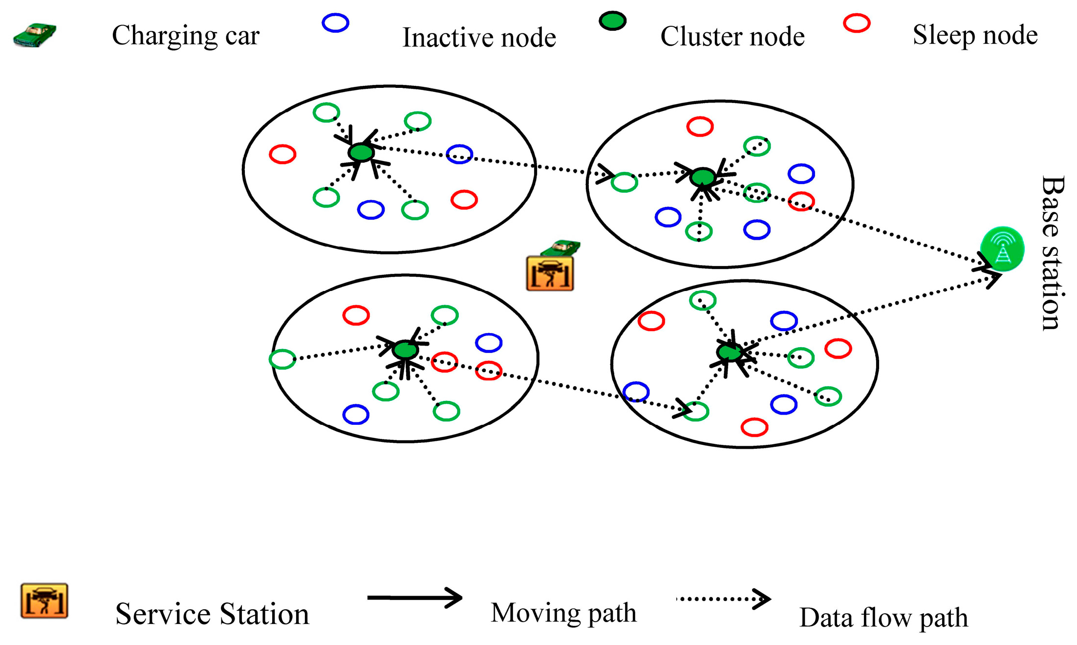
Figure 4.
Network topology in time .

Figure 5.
The graph of charging route.

Figure 6.
Travelling path with 30 sensor nodes.
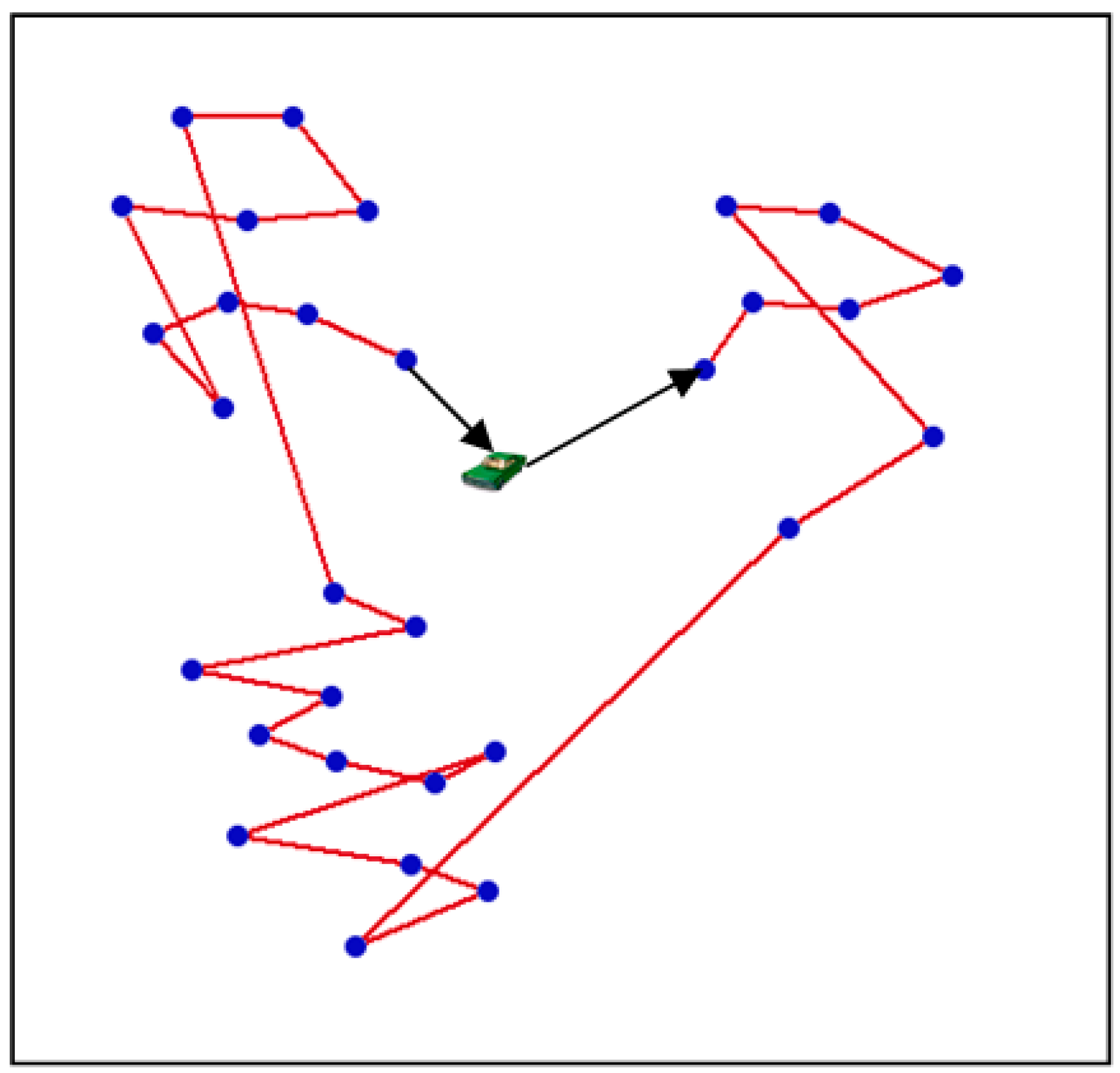
Figure 7.
Travelling path with 40 sensor nodes.
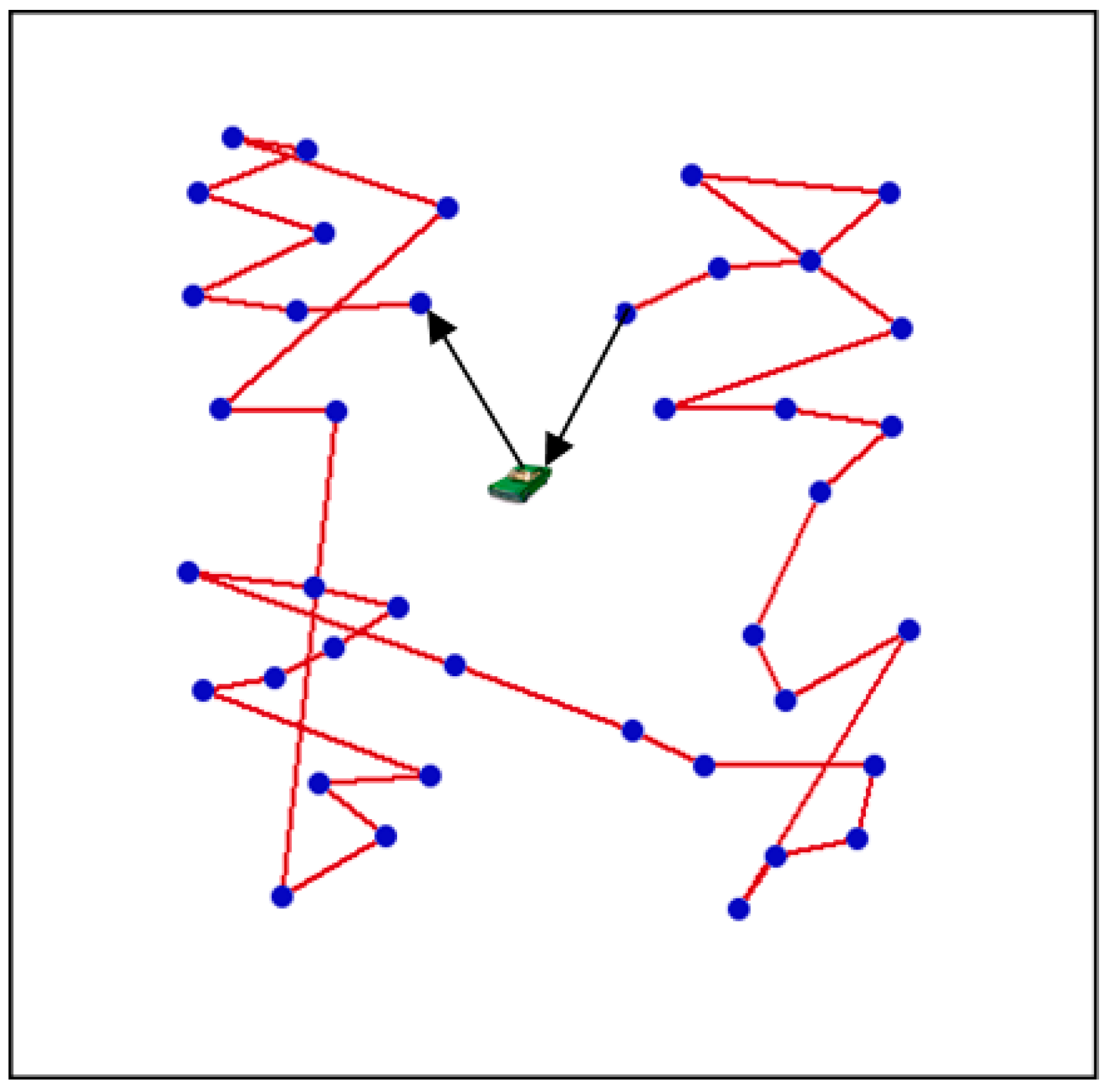
Figure 8.
Travelling path with 50 sensor nodes.

Figure 9.
Travelling path of different scheme.
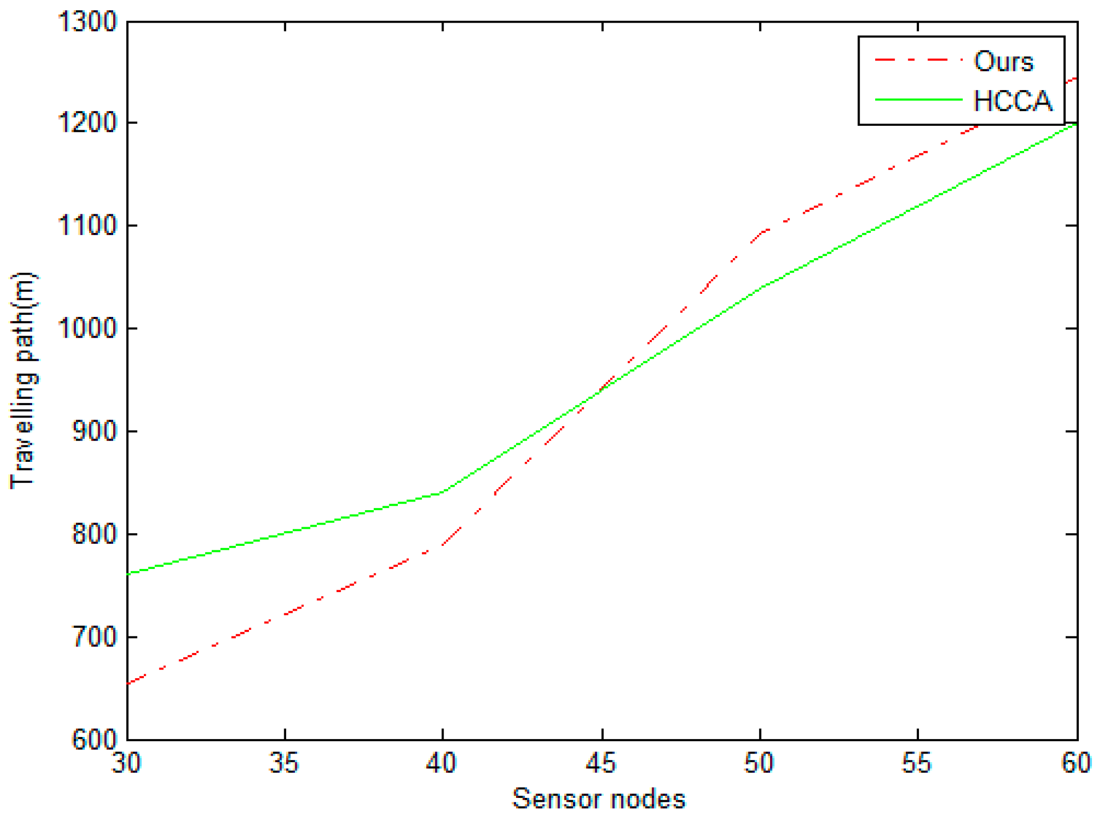
Figure 10.
Recharging time of different scheme.
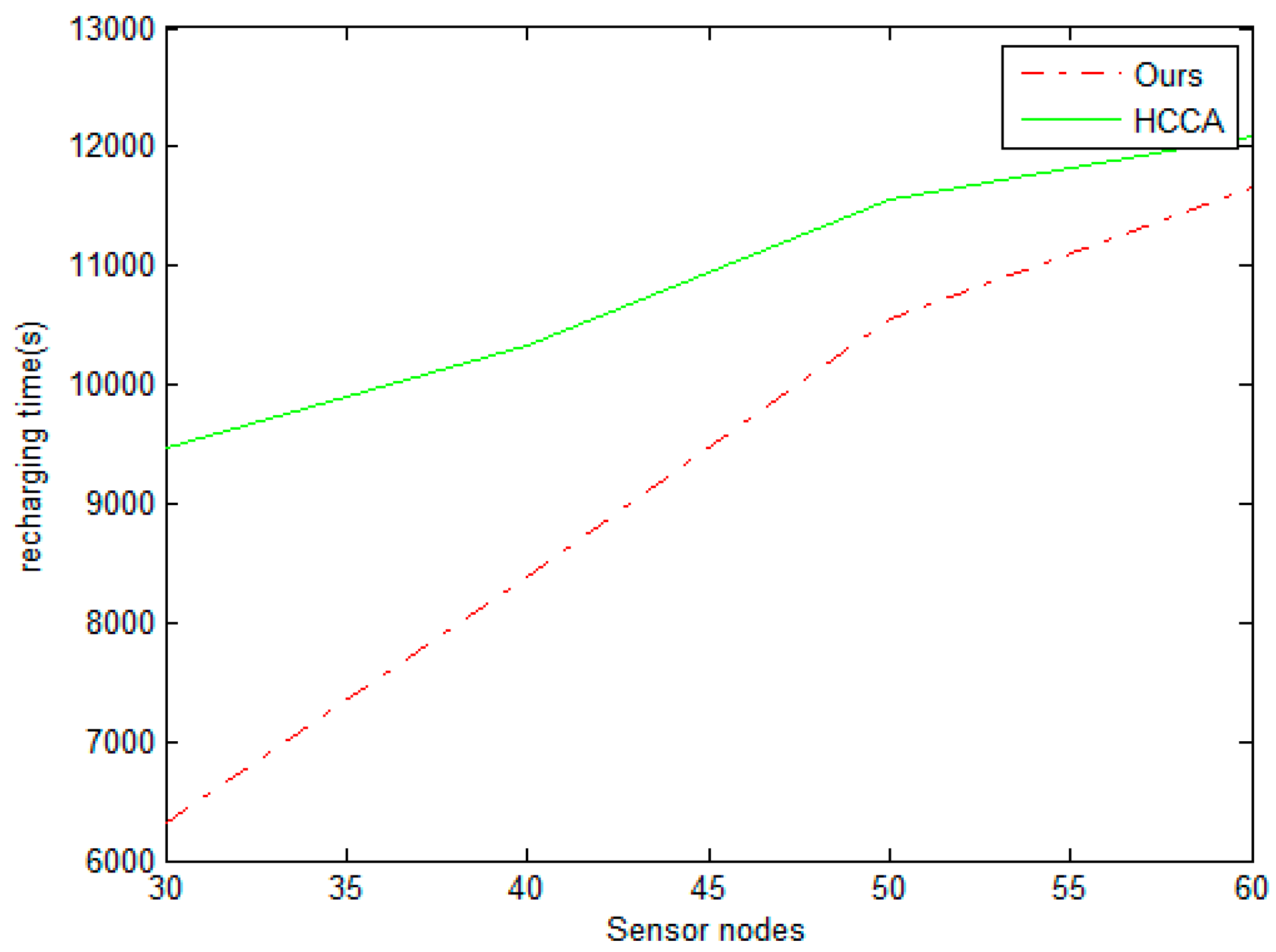
Figure 11.
The change of idle ratio in ours.
© 2017 by the authors. Licensee MDPI, Basel, Switzerland. This article is an open access article distributed under the terms and conditions of the Creative Commons Attribution (CC BY) license (http://creativecommons.org/licenses/by/4.0/).
Share and Cite
MDPI and ACS Style
Wang, Q.; Kong, F.; Wang, M.; Wang, H. Optimized Charging Scheduling with Single Mobile Charger for Wireless Rechargeable Sensor Networks. Symmetry 2017, 9, 285. https://doi.org/10.3390/sym9110285
AMA Style
Wang Q, Kong F, Wang M, Wang H. Optimized Charging Scheduling with Single Mobile Charger for Wireless Rechargeable Sensor Networks. Symmetry. 2017; 9(11):285. https://doi.org/10.3390/sym9110285
Chicago/Turabian StyleWang, Qihua, Fanzhi Kong, Meng Wang, and Huaqun Wang. 2017. "Optimized Charging Scheduling with Single Mobile Charger for Wireless Rechargeable Sensor Networks" Symmetry 9, no. 11: 285. https://doi.org/10.3390/sym9110285
Note that from the first issue of 2016, this journal uses article numbers instead of page numbers. See further details here.