Analytical Treatment of Higher-Order Graphs: A Path Ordinal Method for Solving Graphs


1
Department of Optics, Facultad de Ciencias Físicas, Universidad Complutense de Madrid, Ciudad Universitaria, E-28040 Madrid, Spain
2
Department of Physics, Faculty of Science, Ain Shams University, 1156 Cairo, Egypt
3
Department of Chemical Enginering, E.T.S. de Ingenieros Industriales, Universidad Politécnica de Madrid, C/José Gutiérrez Abascal, 2, E-28006 Madrid, Spain
*
Author to whom correspondence should be addressed.
Symmetry 2017, 9(11), 288; https://doi.org/10.3390/sym9110288
Submission received: 13 October 2017
/
Revised: 17 November 2017
/
Accepted: 17 November 2017
/
Published: 22 November 2017
(This article belongs to the Special Issue Graph Theory)
Abstract
:Analytical treatment of the composition of higher-order graphs representing linear relations between variables is developed. A path formalism to deal with problems in graph theory is introduced. It is shown how paths in the composed graph representing individual contributions to variables relation can be enumerated and represented by ordinals. The method allows for one to extract partial information and gives an alternative to classical graph approach.
1. Introduction
A flow graph is a graphical representation of a system of linear equations. It is introduced by Euler [1], this notion is especially useful in simplifying the treatment of certain linear problems arising e.g., in optical systems [2], classical and quantum field theory [3,4], and network theory [5], just to mention some relevant examples [6]. While this approach is worthy for 2 × 2 systems, for higher-order arrangements it becomes cumbersome. In consequence, to introduce an alternative treatment to solve these higher-order composition graph problems seems to be a relevant task. In this way, some significant contributions were presented earlier [7,8].
Flow graphs are applicable to several fields, such as System of Systems (SoS) implementations. Moreover, higher order graph reduction method could be used as a tool in optimizing the design of SoS, such as, obtaining self-managed smart grids, creating communication networks between all of the possible nodes of systems, setting up a secure transport and auxiliary routes of transportation in real time, managing the energy distribution around systems, permitting flexible and optimized manufacturing, or in financial and business flux analysis.
Flow graph algebra represents a set of linear equations in terms of a complex graph. Through the basic rules, this graph can be reduced to a simpler equivalent form called the “residual graph”. For higher order graphs, there are several paths connecting the input nodes with the output ones, where it results to be difficult to follow a particular trajectory. For this reason, except for in the simplest cases, it is more practical to use numerical methods. Nevertheless, other features of flow graphs are still useful.
Here, we propose a new didactic and intuitive tool to solve graphs in any dimension without reducing them by the conventional rules. The new approach is called Path Ordinal Method (POM). The result is equivalent to a matrix product or graph reduction. However, the utility of the presented method arises in the simplicity of predicting such product graphically by means of a simple calculus table, as well as finding the impact of a certain parameter upon others without solving the entire graph.
The plan of this work is as follows. Section 2.1 is devoted to give a brief overview of the flow graph algebra and the basic reduction rules. In Section 2.2 higher-order graph composition is treated. Each possible path in the graph is defined by an ordinal and its trajectory is characterized by a “path-set”. A new method to solve graphs of any order is introduced showing the way to extract partial information from the composition. Finally, in Section 2.3 we present an application to 3 × 3 matrix composition to demonstrate the validity of the developed method.
2. Materials and Methods
2.1. Flow Graphs
Graphs are geometrical structures that can represent linear equations. They relate magnitudes (variables) by graphic interconnections, following a few rules. A variable is represented by a small circle, called a “node”. White and black colors are used to indicate the orientation of the nodes, which is analogous to the sides of the equation, in standard algebra: black nodes are “sources”, that is, the input variables one has to handle to obtain the output variables called “sinks”, which are indicated by white nodes. The line connecting two nodes is called “branch” and the corresponding label is termed “transmittance”, which indicates that the relation between the interconnected variables. Furthermore, if this transmittance is not specified for a branch, it will be understood that it has the value 1. Branches with transmittance zero are not drawn. Figure 1 shows some flow graph representation of linear equations.
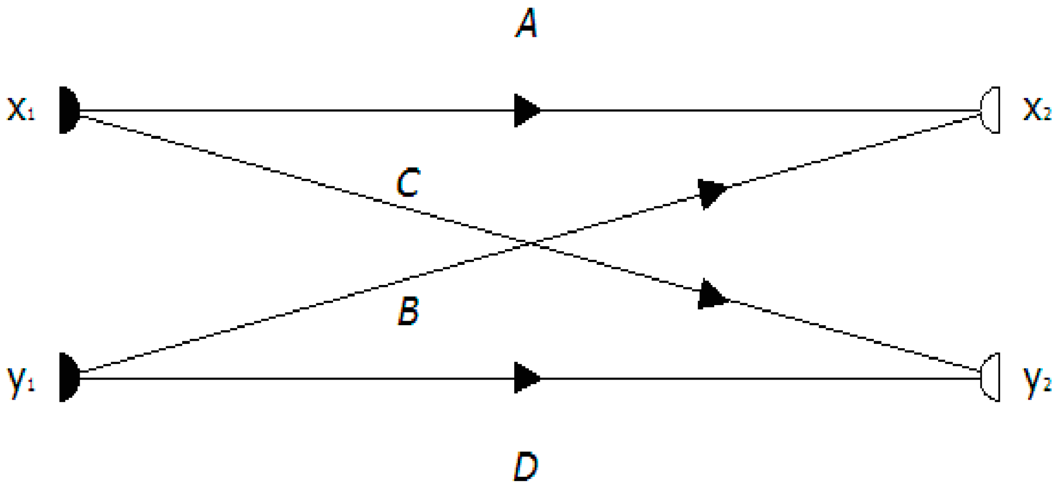
The order of a graph is the smallest number of sources or sinks in the graph. Besides, a cascade graph is the results of the composition of several graphs of the same order. Moreover, there is a mutual relation between matrix representation and flow graphs. For example, the algebraic relation between the following two-dimensional vectors,
can be represented by the second-order graph as in Figure 2.
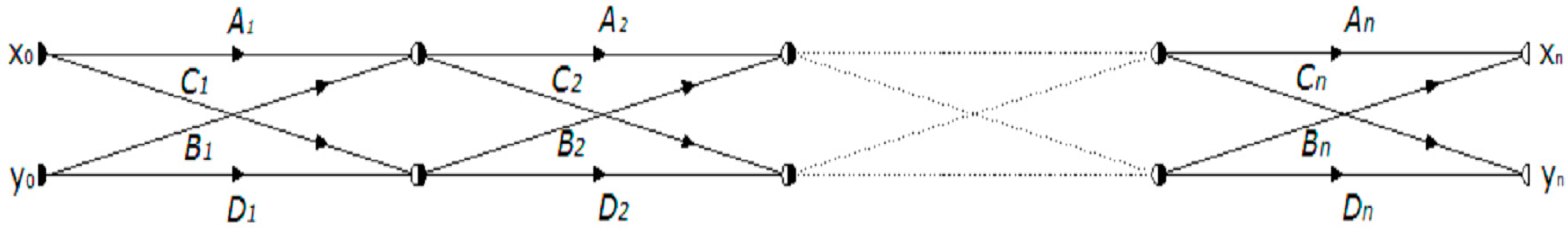
Matrix multiplication can be solved through its alternative graphical representation. Figure 3 shows a composition of n graphs of order two: the result is a cascade graph.
Which is equivalent to the following matrix expression of Equation (2),
For a cascade flow graph there are two ways to proceed. First, by using the five basic algebraic rules namely: addition, product, transmission, suck up node, and self-loop elimination, where an equivalent simpler graph is obtained. The second one is the Mason’s rule, recommended when we are only interested in one of the output variables as a function of one of the input variables.
2.2. Graph Composition and Path Characterization
The analysis of bulky systems made of several elements implies the composition of higher-order graphs, which turns to be complicated. In this section, we propose a general method to obtain the equivalent matrix, as well as the residual graph directly from the individual elements. Also, the influence of a certain input parameters upon an output one could be obtained without solving the whole graph.
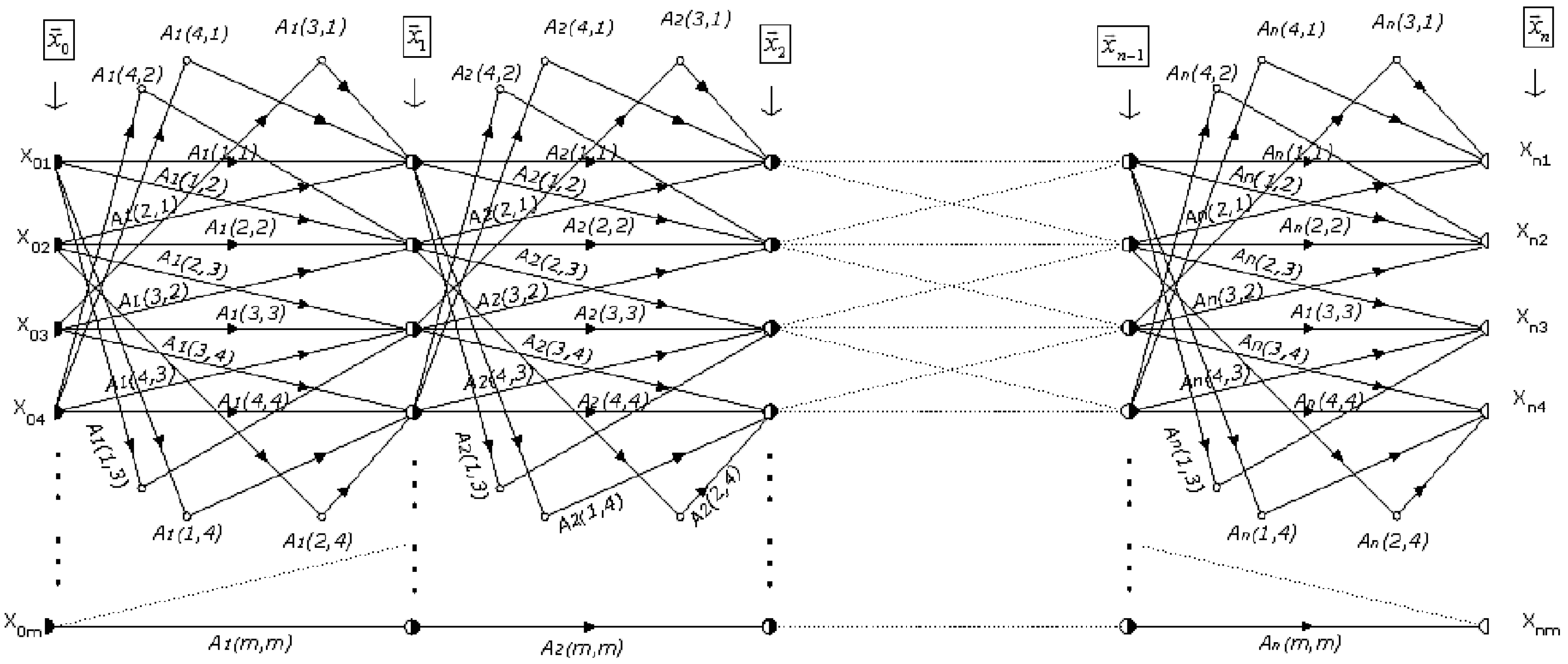
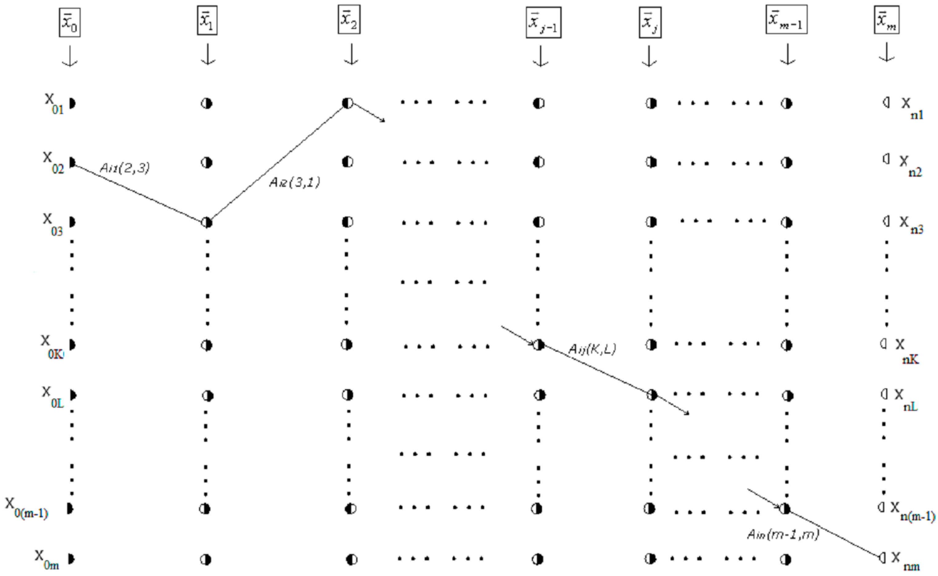
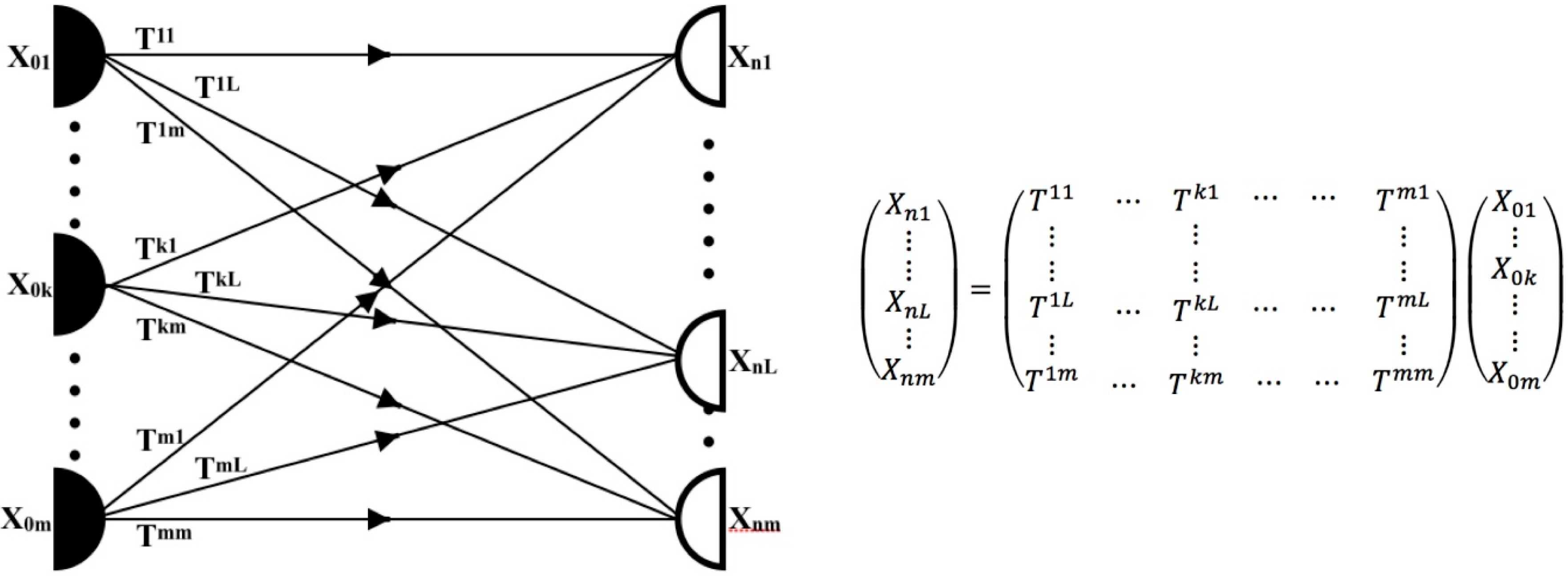
We define two graphs: the cascade graph representing the whole system and the individual graph corresponding to any arbitrary element of the system. Consider, for example, the cascade graph of Figure 4.
The input variables are the vector:
and the output variables are represented by the vector:
This cascade graph is composed of n graphs, attached side by side, each one of order m. In consequence, the total number of possible paths connecting the input nodes to the output ones is:
Nm,n = mn+1.
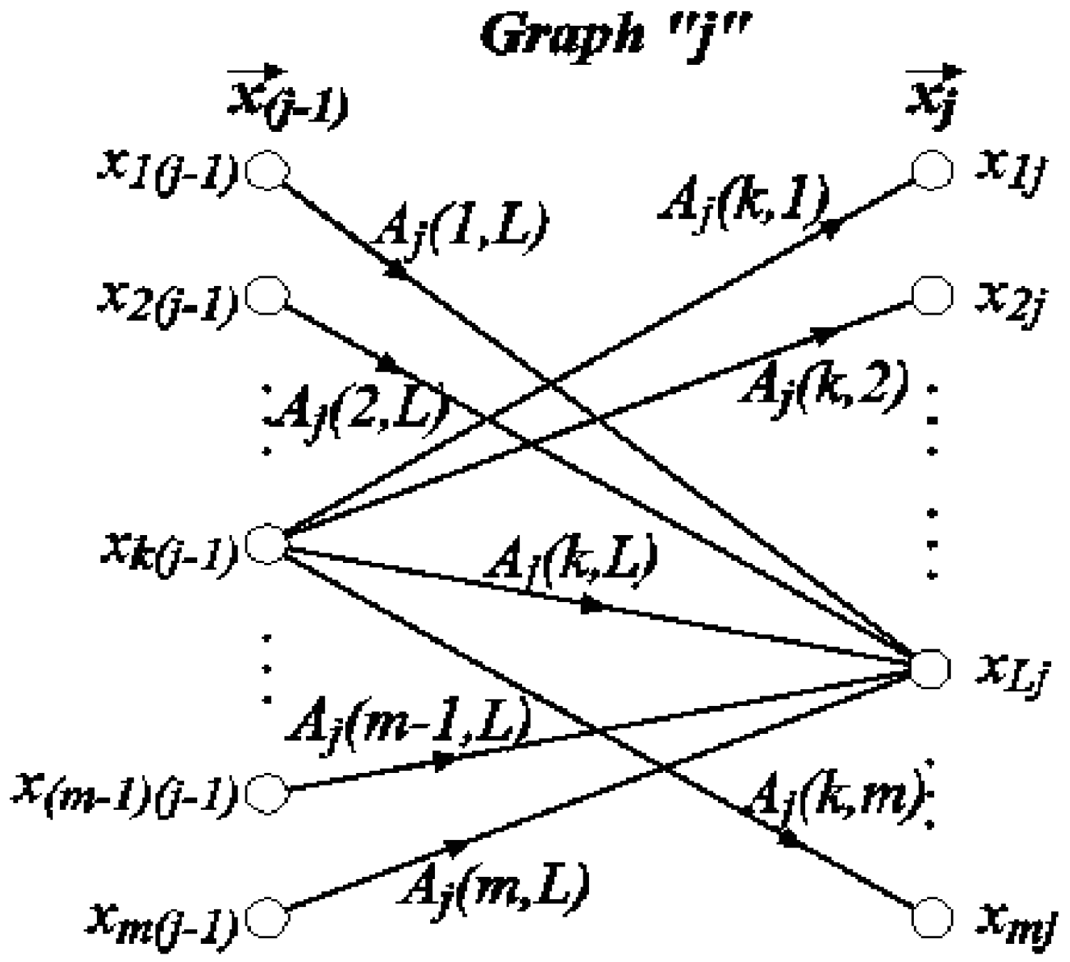
Now, let us consider the jth constituent of the cascade graph as sketched in Figure 5.
The total number of possible paths is m2. This individual graph is defined by the incoming nodes vector and the outgoing nodes vector , where j takes the values j = 1, 2, 3, …, n.
2.2.1. Ordinal of a Path and Path Value
An arbitrary path with an ordinal i (1 ≤ i ≤ Nm,n), connecting any node in the input vector with another node in the output vector, is characterized by a set of numbers {θij} that we will call “path-set”, which defines the trajectory of the path.
These θij can take any of the values 1 ≤ θij ≤ m. If θij = k this means that the ith path passes through the kth node of the jth vector, xjk. An example of a path-set is illustrated in Figure 6.
The value of any possible path Pi can be seen as the product of the transmittances corresponding to each branch along the path
where Aij is the transmittance of the branch in the jth graph within the path i (see Figure 5).
Separating the contribution of the first and the last graph we get:
The path value Pi that starts in an arbitrary node x0k in the input vector and reaches the output vector in any arbitrary node xnL, is given by
So, each path is defined by two items, the path ordinal i and the path value , where both are associated to a “path-set”.
Defining a path sequence, the first path (i = 1) will start from the node x01 and will end at the node xn1, the second starts from the node x02 and ends at the node xn1, the kth will start from the node x0k till the path m is reached, which starts from the node x0m and ends at the node xn1.
When considering the output vector as it is composed of m outgoing nodes. The total number of paths Nm,n is divided into m groups each has mn paths. The first group ends at the node x1n where (1 ≤ i ≤ mn) and the second group ends at the node xn2 where (1 + mn ≤ i ≤ 2mn). As a consequence, all of the paths that end at the node xnL have the path ordinals within the limit (1 + (L − 1)mn ≤ i ≤ Lmn). On the other hand, all of the paths that start from the node x0k, according to the path sequence, have the ordinals i = k, k + m, k + 2m, ….
Thus, for a m × n cascade graph, there are mn−1 paths connecting an output node with an input one. These paths that start from an input node x0k and ends at an output node xnL, have the path ordinals i = k + (L − 1)mn, k + m+ (L − 1)mn, …, k – m + Lmn.
The contribution of the source x0k to the sink xnL, can be expressed as the summation of all the paths that start from x0k and end at xnL as follows,
Similarly, the total contribution of the input vector nodes to the sink xnL is given by,
Calling TkL to the summation of all the path values that start from x0k and end at xnL
So, the sink xnL can be expressd as,
Hence, for a m × n graph, the contribution of all the sources to all of the sinks, can be represented by the equation:
According to Equation (3) for all of the path-sets representing such trajectories, only θi0 and θin are defined, with the values k and L, respectively. Now, the goal is to define the trajectory of an arbitrary path, i.e., to evaluate the set of numbers {θij}.
2.2.2. Determination of the Characteristic Path Set
As it is mentioned before, for a cascade graph, there are m groups of paths, of which, each is composed mn paths. Each group reaches an output node. Accordingly, the group of paths that reaches an arbitrary node xnL in the output vector has the path ordinals within the range (1 + (L − 1)mn ≤ i ≤ Lmn).
Proceeding to calculate the path set. For any path of ordinal i, if the path ordinal i is subtracted by one and then divided by the number of paths that reach an output node (mn), we get:
where mn is de divisor, Cn is the quotient (0 ≤ Cn < m), and Rn is the reminder (0 ≤ Rn < mn). So, the last element of the path-set θin can be expressed as:
Similarly the penultimate element of the path set is calculated by considering a cascade graph of n − 1 graphs each of order m. The total number of paths corresponding to such graph is mn−1 paths. Now, the path ordinal becomes:
i = Rn + 1.
To determine the node x(n−1)L that the path ends at, following the previous procedure, the path ordinal is subtracted by one and then divided by mn−1, so we have:
where 0 ≤ Cn−1 < m and 0 ≤ Rn−1 < mn−1. Iterating the same procedure, we finally get:
On account of this:
Thus, we conclude that, for a given path-ordinal i the corresponding path-set {θij} can be determined as follows:
- I
- The path ordinal is subtracted by one.
- II
- Then, it is divided by m for n-times.
- III
- Finally, one is added to the remainders of the division, R1, C1, C2, …, Cn.
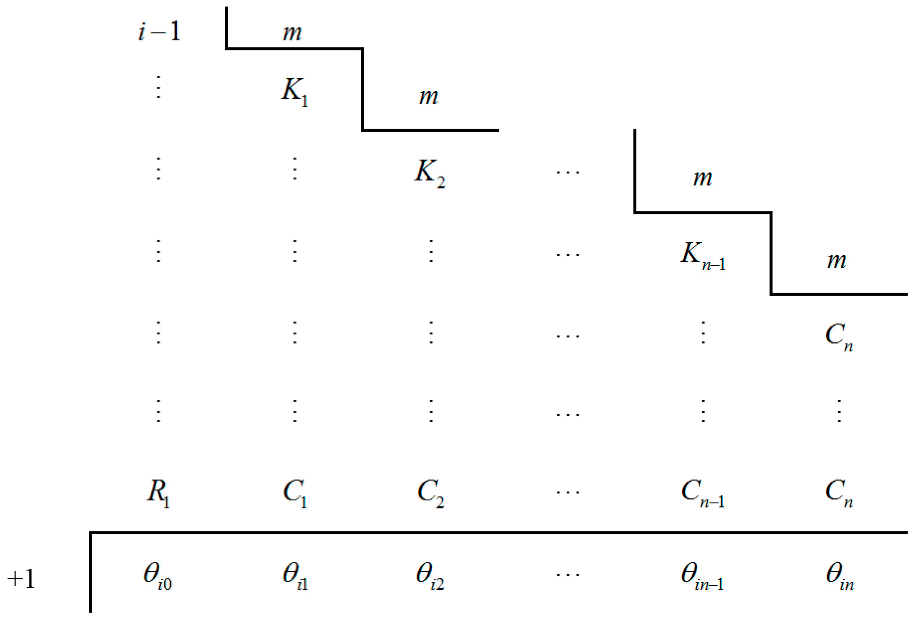
A scheme illustrating the calculation of the path-set is shown in the next diagram Figure 7.
The utility of the Path Set Diagram (PSD) is crucial in the application of Equations (7)–(9). In the next section, we discuss a simple and explicit example to illustrate how the Path Ordinal Method (POM) works.
2.3. Examples and Concluding Remarks
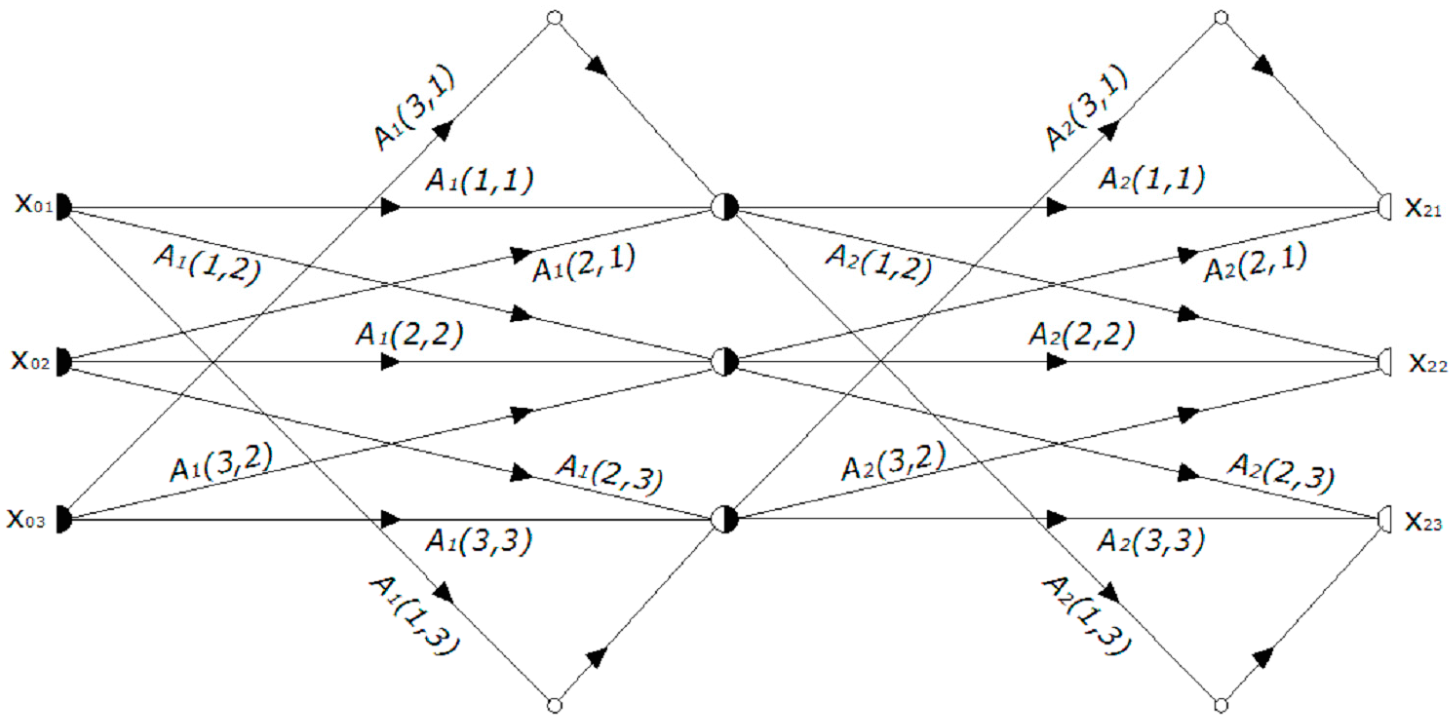
Consider an arbitrary system that is composed of two elements, each one is represented by a 3 × 3 matrix. Starting from the physical scheme of the system, the flow graph is formed by attaching side by side the graph corresponding to each element. The result is a 3 × 2 cascade graph. The cascade graph of the problem is shown the Figure 8.
The problem can be solved either by matrix multiplication as in Equation (12) or through conventional graph reduction rules.
However, we will proceed to get the residual graph as well as the equivalent matrix by applying the POM. We denote the equivalent matrix as:
Using the path ordinal formalism we will find the partial contribution of an input parameter, as well as the total solution.
2.3.1. The Contribution of and Input Parameter to an Output Parameter
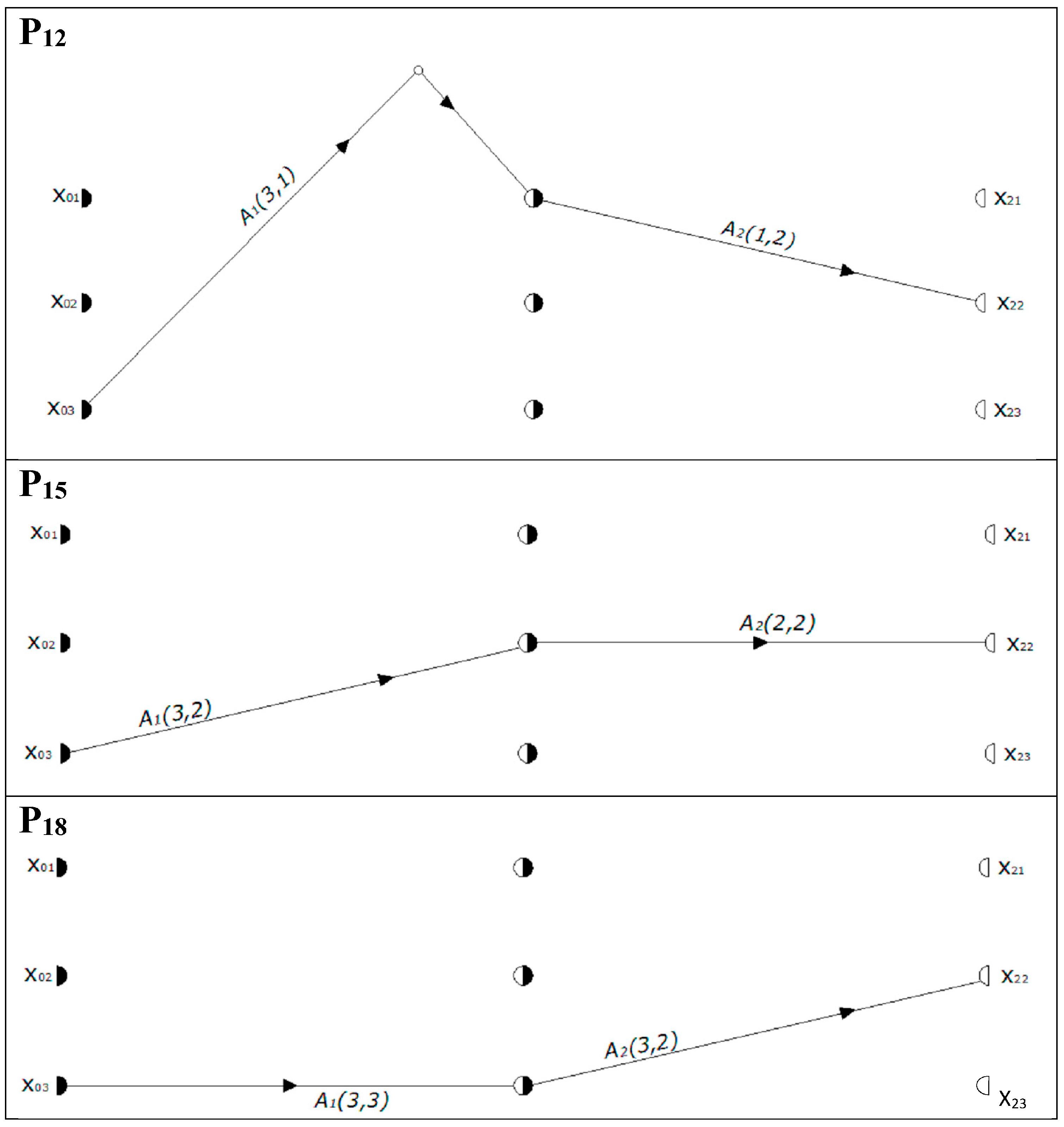
If one is interested to know the effect of an input parameter on an output one, it is not necessary to build the whole matrix or to reduce the whole graph. When considering the path sequence, the contribution of e.g., the input parameter x03 to the output parameter x22 is given by the matrix element T32. When applying Equation (8), we get:
Accordingly, there are three paths that connect both nodes. These paths have the ordinals 12, 15, and 18. The path-values of the above equation are calculated by specifying, firstly, the path-set corresponding to each trajectory.
For the paths of ordinals 12, 15, and 18, the corresponding path sets are obtained by means of the PSD as follows:
| 12 − 1 = | 11 | 3 | 15 − 1 = | 14 | 3 | 18 − 1 = | 17 | 3 | |||||
| : | 3 | 3 | : | 4 | 3 | : | 5 | 3 | |||||
| : | : | 1 | : | : | 1 | : | : | 1 | |||||
| : | : | : | : | : | : | : | : | : | |||||
| 2 | 0 | 1 | 2 | 1 | 1 | 2 | 2 | 1 | |||||
| +1 | 3 | 1 | 2 | +1 | 3 | 2 | 2 | +1 | 3 | 3 | 2 |
For completeness, the corresponding graph-trajectories according to the above calculations appear in Figure 9.
Hence, we get,
We emphasize that, by means of the POM and as an alternative to the classical approach, we have simply obtained a matrix element without solving the whole matrix product or reducing the whole graph. This is precisely one of the applications of the formalism.
2.3.2. The Total Solution
The cascade graph is solved by specifying the equivalent matrix of the system. In consequence, the residual graph can be drawn easily. According to Equation (10) and recalling Equation (12), the algebraic expression representing the system is
The equivalent matrix elements are calculated through three steps, each is represented within a table. The path-sets corresponding to each possible path is illustrated in Table 1, while Table 2 gives the path values corresponding to the path sets of Table 1.
The matrix elements are calculated according to Equation (8) and represented in Table 3.
Obtaining the matrix elements, which are homologues to the graph transmittances, the residual graph could be drawn easily.
In summary, what we expect to have accomplished is to work out a new didactic and useful tool to solve graphs of different dimensions as an alternative to reducing them by the conventional rules.
3. Results and Discussion
A new didactic, simple, and intuitive tool is developed. The POM is applicable to any type of problems that could be raised with the usual matrix algebra or graphs of any order, contributing an alternative and powerful treatment that allows for treating multitude of problems in physics that nowadays are approached by means of standard matrix treatment or flow graph algebra.
The aptitude of the method to treat as an independent form, each of the contributions of the different components of the input and output vectors, is especially useful in problems of Physics in which one is interested in knowing the impact of certain input parameter of the problem on others. Also, the utility of the method could be observed in problems with higher order matrix compositions or higher order graphs.
The POM states that; for any arbitrary cascade graph represented by the input variables vector
and the output variables vector
there exist possible paths connecting the input nodes with the output ones (Figure 4). These paths are defined by an ordinal (1 ≤ i ≤ Nm,n), which, as a consequence, is attached to a characteristic Path-Set that determines the path along the graph and a Path-Value that is considered as the product of the transmittances corresponding to each branch along the path. Once the path values are calculated, the transmittances of the branches of the residual graph are calculated through Equation (8), which are homologues to the matrix elements representing the system. For better organization, simplicity, and in order to avoid calculation mistakes, we suggest that all of the calculations to be put in tables. Table 4 and Table 5, and Figure 10 summarizes the process.
In addition, a useful feature of the POM is its practicability in special problems when the impact of a certain parameter upon others is of our interest. Taking into account the path order, the contribution of a source x0k to a sink xnL is given by the transmittance TkL of the residual graph. Which is the summation of its corresponding path values in agreement with Equation (8). These path values can be calculated directly by specifying their corresponding path sets by means of the PSD illustrated in Figure 7, i.e., by applying the POM the contribution of a source to a sink can be calculated easily without solving the entire problem.
The fields of application of this tool spread to all of those linear problems that are treated in physics by means of matrix algebra or flow graphs, being especially effective in the simplification of some specific calculations possessing composition of several high order matrices or bulky graphs.
Clear examples of applications could be fields as: matrix optics in asymmetric systems, matrix treatments in quantum mechanics and quantum theory of fields, treatments of dielectric multilayers, analysis of tensor mechanical properties of materials, optical networks, classic mechanics formulations, polarization and depolarization problems in optics, fluids dynamics, acoustic, and in general, any problem that holds linear relations and sets the stage for a matrix treatment. The POM was applied to 3-layers dielectric system [9].
Finally, other industrial applications could be the simulation in designing System of Systems focused on communication networks, multimodal traffic control, energy distribution systems, multi-site industrial manufacture or emergency management, among others.
Acknowledgments
This work has been funded by the European Commission within the 7th Framework Program and the project “ReBorn–Innovative re-use of modular equipment based on integrated factory design”, Grant Agreement No. 609223. Also, below the support of SEGVAUTO-TRIES-CM Program P2013-MIT-2713. The authors would like to express their gratitude to Eduardo Martin-Martinez for his preliminary help at the beginning of this research.
Author Contributions
Hala Kamal analyzed the problem, done all the mathematical calculations, derived the achieved method and wrote the paper. Eusebio Bernabeu directed the work pointing out the tools to be used and revised the paper. Alicia Larena oriented the selection of some input/output parameters in relation to possible realistic applications in future works. She has done a critical analysis of the manuscript.
Conflicts of Interest
The authors declare no conflict of interest.
References
- Euler, L. The Seven Bridges of Konigsberg. Comment. Acad. Sci. Imp. Petropolitanae 1741, 8, 128–140. [Google Scholar]
- Wang, S.; Zhao, D. Matrix Optics; Zhejiang University Press: Hangzhou, China, 2000. [Google Scholar]
- Feynman, R.P. Quantum Electrodynamics; Perseus: New York, NY, USA, 1998. [Google Scholar]
- Peskin, M.E.; Schroeder, D.V. Quantum Field Theory; Perseus: New York, NY, USA, 1995. [Google Scholar]
- Weissman, Y. Optical Network Theory; Artech: New York, NY, USA, 1992. [Google Scholar]
- Bondy, J.A.; Murty, U.S.R. Graph Theory with Applications; North-Holland: Oxford, UK, 1976. [Google Scholar]
- Coates, C.L. Flow—Graph Solutions of Linear Algebric Equations. IRE Trans. Circuit Theory 1959, 6, 170–187. [Google Scholar] [CrossRef]
- Chen, W.-K. On Flow graph Solutions of Linear Algebric Equations. SIAM J. Appl. Math. 1967, 15, 136–142. [Google Scholar] [CrossRef]
- Kamal, H.; Bernabeu, E. High order graph formalism for multilayer structures. Opt. Int. J. Light Electron Opt. 2016, 127, 1384–1390. [Google Scholar] [CrossRef]
Figure 1.
Elementary graph-algebra operations.
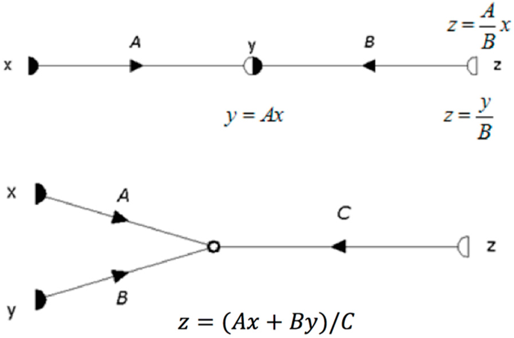
Figure 2.
A second order graph representing Equation (1). The homologous of the vector parameters are the nodes while the homologous of the matrix elements are the branches transmittance.
Figure 2.
A second order graph representing Equation (1). The homologous of the vector parameters are the nodes while the homologous of the matrix elements are the branches transmittance.

Figure 3.
A cascade graph composed of n graphs of order two, attached side by side. Each individual graph represents a 2 × 2 matrix.
Figure 3.
A cascade graph composed of n graphs of order two, attached side by side. Each individual graph represents a 2 × 2 matrix.

Figure 4.
A m × n cascade graph.

Figure 5.
The jth graph of order m inside the cascade graph of Figure 4. Aj(k,L) represents the transmittance of the branch connecting the nodes xk and xL.
Figure 5.
The jth graph of order m inside the cascade graph of Figure 4. Aj(k,L) represents the transmittance of the branch connecting the nodes xk and xL.

Figure 6.
An example illustrating a path i. The trajectory of the path corresponds to the path-set {θij} = {2,3,1,…,k,L,…,m − 1,m} where xmn = Pix20 and Pi = (A1(2,3)·A1(3,1)·…Aj(k,L)·…An(m − 1,m)).
Figure 6.
An example illustrating a path i. The trajectory of the path corresponds to the path-set {θij} = {2,3,1,…,k,L,…,m − 1,m} where xmn = Pix20 and Pi = (A1(2,3)·A1(3,1)·…Aj(k,L)·…An(m − 1,m)).

Figure 7.
The Path Set Diagram (PSD). Starting from a path ordinal 𝑖, its corresponding characteristic path set is calculated as follows: firstly, the path ordinal is subtracted by one, then it is divided by m n-times, finally one is added to the remainders of the division.
Figure 7.
The Path Set Diagram (PSD). Starting from a path ordinal 𝑖, its corresponding characteristic path set is calculated as follows: firstly, the path ordinal is subtracted by one, then it is divided by m n-times, finally one is added to the remainders of the division.

Figure 8.
A cascade graph resulting from the composition of two graphs of order 3.

Figure 9.
The three possible graph paths P12, P15, and P18, connecting the input node x03 to the output node x22 according to the path sets calculated by the Path Set Diagram (PSD).
Figure 9.
The three possible graph paths P12, P15, and P18, connecting the input node x03 to the output node x22 according to the path sets calculated by the Path Set Diagram (PSD).

Figure 10.
The residual graph and its equivalent matrix form.


Table 1.
The path-sets corresponding to the 3 × 2 cascade graph. The table is divided vertically into three parts, each part represents the paths that reach the output nodes x21, x22 and x23, respectively.
Table 1.
The path-sets corresponding to the 3 × 2 cascade graph. The table is divided vertically into three parts, each part represents the paths that reach the output nodes x21, x22 and x23, respectively.
| i | θi0 | θi1 | θi2 | i | θi0 | θi1 | θi2 | i | θi0 | θi1 | θi2 | ||
|---|---|---|---|---|---|---|---|---|---|---|---|---|---|
| 1 | 1 | 1 | 1 | 10 | 1 | 1 | 2 | 19 | 1 | 1 | 3 | ||
| 2 | 2 | 1 | 1 | 11 | 2 | 1 | 2 | 20 | 2 | 1 | 3 | ||
| 3 | 3 | 1 | 1 | 12 | 3 | 1 | 2 | 21 | 3 | 1 | 3 | ||
| 4 | 1 | 2 | 1 | 13 | 1 | 2 | 2 | 22 | 1 | 2 | 3 | ||
| 5 | 2 | 2 | 1 | 14 | 2 | 2 | 2 | 23 | 2 | 2 | 3 | ||
| 6 | 3 | 2 | 1 | 15 | 3 | 2 | 2 | 24 | 3 | 2 | 3 | ||
| 7 | 1 | 3 | 1 | 16 | 1 | 3 | 2 | 25 | 1 | 3 | 3 | ||
| 8 | 2 | 3 | 1 | 17 | 2 | 3 | 2 | 26 | 2 | 3 | 3 | ||
| 9 | 3 | 3 | 1 | 18 | 3 | 3 | 2 | 27 | 3 | 3 | 3 |
Table 2.
The path values corresponding to the path-sets of Table 1.
Table 2.
The path values corresponding to the path-sets of Table 1.
| Pi | Path Value | Pi | Path Value | Pi | Path Value |
|---|---|---|---|---|---|
| P1 | A1(1,1)*A2(1,1) | P10 | A1(1,1)*A2(1,2) | P19 | A1(1,1)*A2(1,3) |
| P2 | A1(2,1)*A2(1,1) | P11 | A1(2,1)*A2(1,2) | P20 | A1(2,1)*A2(1,3) |
| P3 | A1(3,1)*A2(1,1) | P12 | A1(3,1)*A2(1,2) | P21 | A1(3,1)*A2(1,3) |
| P4 | A1(1,2)*A2(2,1) | P13 | A1(1,2)*A2(2,2) | P22 | A1(1,2)*A2(2,3) |
| P5 | A1(2,2)*A2(2,1) | P14 | A1(2,2)*A2(2,2) | P23 | A1(2,2)*A2(2,3) |
| P6 | A1(3,2)*A2(2,1) | P15 | A1(3,2)*A2(2,2) | P24 | A1(3,2)*A2(2,3) |
| P7 | A1(1,3)*A2(3,1) | P16 | A1(1,3)*A2(3,2) | P25 | A1(1,3)*A2(3,3) |
| P8 | A1(2,3)*A2(3,1) | P17 | A1(2,3)*A2(3,2) | P26 | A1(2,3)*A2(3,3) |
| P9 | A1(3,3)*A2(3,1) | P18 | A1(3,3)*A2(3,2) | P27 | A1(3,3)*A2(3,3) |
Table 3.
The matrix elements corresponding to the example, according to 3 × 2 graph analysis.
| T11 = P1 + P4 + P7 | T21 = P2 + P5 + P8 | T31 = P3 + P6 + P9 |
| T12 = P10 + P13 + P16 | T22 = P11 + P14 + P17 | T32 = P12 + P15 + P18 |
| T13 = P19 + P22 + P25 | T23 = P20 + P23 + P26 | T33 = P21 + P24 + P27 |
Table 4.
A general form of a table used to calculate all the possible paths of a cascade graph. Aj(k,L) represents the transmittance of the branch connecting the node X(j − 1)k and Xjk in the jth graph.
Table 4.
A general form of a table used to calculate all the possible paths of a cascade graph. Aj(k,L) represents the transmittance of the branch connecting the node X(j − 1)k and Xjk in the jth graph.
| Path Ordinal Pi | Path Set | Path Value |
|---|---|---|
| 1 | {1, 1…………...…..., 1} | P1 = A1(1,1)*………………An(1,1) |
| : | : | : |
| mn | {m, m…………….…, 1} | = A1(m,m)*………….An(m,1) |
| : | : | : |
| : | : | : |
| mn+1 | {m, m……………..., m} | = A1(m,m)*………...An(m,m) |
Table 5.
A table illustrating the value of each transmittance in the residual graph as a sum of its corresponding path-values.
Table 5.
A table illustrating the value of each transmittance in the residual graph as a sum of its corresponding path-values.
| … | … | |||
| : : | … | : : | … | : : |
| … | … | |||
| : : | … | : : | … | : : |
| … | … |
© 2017 by the authors. Licensee MDPI, Basel, Switzerland. This article is an open access article distributed under the terms and conditions of the Creative Commons Attribution (CC BY) license (http://creativecommons.org/licenses/by/4.0/).
Share and Cite
MDPI and ACS Style
Kamal, H.; Larena, A.; Bernabeu, E. Analytical Treatment of Higher-Order Graphs: A Path Ordinal Method for Solving Graphs. Symmetry 2017, 9, 288. https://doi.org/10.3390/sym9110288
AMA Style
Kamal H, Larena A, Bernabeu E. Analytical Treatment of Higher-Order Graphs: A Path Ordinal Method for Solving Graphs. Symmetry. 2017; 9(11):288. https://doi.org/10.3390/sym9110288
Chicago/Turabian StyleKamal, Hala, Alicia Larena, and Eusebio Bernabeu. 2017. "Analytical Treatment of Higher-Order Graphs: A Path Ordinal Method for Solving Graphs" Symmetry 9, no. 11: 288. https://doi.org/10.3390/sym9110288
Note that from the first issue of 2016, this journal uses article numbers instead of page numbers. See further details here.