New Applications of m-Polar Fuzzy Matroids


Department of Mathematics, University of the Punjab, New Campus, Lahore 54590, Pakistan
*
Author to whom correspondence should be addressed.
Symmetry 2017, 9(12), 319; https://doi.org/10.3390/sym9120319
Submission received: 1 November 2017
/
Revised: 7 December 2017
/
Accepted: 11 December 2017
/
Published: 18 December 2017
(This article belongs to the Special Issue Fuzzy Techniques for Decision Making)
Abstract
:Mathematical modelling is an important aspect in apprehending discrete and continuous physical systems. Multipolar uncertainty in data and information incorporates a significant role in various abstract and applied mathematical modelling and decision analysis. Graphical and algebraic models can be studied more precisely when multiple linguistic properties are dealt with, emphasizing the need for a multi-index, multi-object, multi-agent, multi-attribute and multi-polar mathematical approach. An m-polar fuzzy set is introduced to overcome the limitations entailed in single-valued and two-valued uncertainty. Our aim in this research study is to apply the powerful methodology of m-polar fuzzy sets to generalize the theory of matroids. We introduce the notion of m-polar fuzzy matroids and investigate certain properties of various types of m-polar fuzzy matroids. Moreover, we apply the notion of the m-polar fuzzy matroid to graph theory and linear algebra. We present m-polar fuzzy circuits, closures of m-polar fuzzy matroids and put special emphasis on m-polar fuzzy rank functions. Finally, we also describe certain applications of m-polar fuzzy matroids in decision support systems, ordering of machines and network analysis.
Keywords:
m-polar fuzzy matroid; m-polar fuzzy uniform matroid; m-polar fuzzy linear matroid; m-polar fuzzy partition matroid; m-polar fuzzy cycle matroid; m-polar fuzzy rank function; closure; m-polar fuzzy circuitMSC:
05C65; 05C85; 05C90; 03E721. Introduction
Matroid theory had its foundations laid in 1935 after the work of Whitney [1]. This theory constitutes a useful approach for linking major ideas of linear algebra, graph theory, combinatorics and many other areas of Mathematics. Matroid theory has been a focus of active research during the last few decades.
Zadeh’s fuzzy set theory [2,3] handles real life data having non-statistical uncertainty and vagueness. Petković et al. [4] investigated the accuracy of an adaptive neuro-fuzzy computing technique in precipitation estimation. Various applications of fuzzy sets in the field of automotive and railway level crossings for safety improvements are studied in [5,6]. The fuzzy set plays a vital role to solve various multi-criteria decision making problems. Some applications of fuzzy theory in multi-criteria models are discussed in [7,8]. Zhang [9] extended fuzzy set theory to bipolar fuzzy sets and discusses the bipolar behaviour of objects. The idea which lies behind such a description is connected with the existence of “bipolar information”. For illustration, profit and loss, hostility and friendship, competition and cooperation, conflicted interests and common interests , unlikelihood and likelihood, feedback and feedforward, and so on, are generally two sides in coordination and decision making. Just like that, bipolar fuzzy set theory indeed has considerable impacts on many fields, including computer science, artificial intelligence, information science, decision science, cognitive science, economics, management science, neural science, medical science and social science. Recently, bipolar fuzzy set theory has been applied and studied speedily and increasingly. Thus, bipolar fuzzy sets not only have applications in mathematical theories but also in real-world problems [10,11,12].
In a number of real world problems, data come from m sources or agents , that is, multi-indexed information arises which cannot be mathematically expressed by means of the existing approaches of classical set theory, the crisp theory of graphs, fuzzy systems and bipolar fuzzy systems. The research presented in this paper is mainly developed to handle the lack of a mathematical approach towards multi-index, multipolar and multi-attribute data. Nowadays, analysts believe that the natural world is approaching the ideas of multipolarity. Multipolarity in data and information plays an important role in various domains of science and technology. In information technology, multipolar technology can be oppressed to operate large scale systems. In neurobiology, multipolar neurons in brain assemble a lot of information from other neurons. For instance, over a noisy channel, a communication channel may have a different network range, radio frequency, bandwidth and latency. In a food web, species may be of different types including strong, weak, vegetarian and non-vegetarian, and preys may be energetic, harmful and digestive. In a social network, the influence rate of different people may be different with respect to socialism, proactiveness, and trading relationship. A company may have different market power from others according to its product quality, annum profit, price control of its product, etc. These are multipolar information which are fuzzy in nature. To discuss such network models, we need mathematical and theoretical approaches which deal with multipolar information.
In view of this motivation, Chen et al. [13] extended bipolar fuzzy set theory and introduced the powerful idea of m-polar fuzzy sets. The membership value of an object, in an m-polar fuzzy set, belongs to , which represents m different attributes of the object. Considering the idea of graphic structures, -polar fuzzy sets can be used to describe the relationship among several individuals. In particular, m-polar fuzzy sets have found applications in the adaptation of accurate problems if it is necessary to make decisions and judgements with a number of agreements. For instance, the exact value of telecommunication safety of human beings is a point which lies in , since different people are monitored in different times. Some other applications include ordering and evaluation of alternatives and m-valued logic. m-polar fuzzy sets are shown to be useful to explore weighted games, cooperative games and multi-valued relations. In decision making issues, m-polar fuzzy sets are helpful for multi-criteria selection of objects in view of multipolar data. For example, m-polar fuzzy sets can be implemented when a country elects its political leaders, a company decides to manufacture an item or product, a group of friends wants to visit a country with multiple alternatives. In wireless communication, it can be used to discuss the conflicts and confusions of communication signals. Thus, m-polar fuzzy sets not only have applications in mathematical theories but also in real-world problems.
Akram and Younas [14] implemented the concept of m-polar fuzzy set into graph theory and discussed irregularity in m-polar fuzzy graphs. Several researchers have been applying this technique to explore various applications of m-polar fuzzy theory including grouping of objects [15], detecting human trafficking suspects [16], finding minimum number of locations [17] and decision support systems [18]. In 1988, Goetschel [19] studied the approach to the fuzzification of matroids and discussed the uncertain behaviour of matroids. The same authors [20] introduced the concept of bases of fuzzy matroids, fuzzy matroid structures and greedy algorithm in fuzzy matroids. Akram and Sarwar [15,21] have also discussed m-polar fuzzy hypergraphs, product formulae of distance for various types of m-polar fuzzy graphs and applications of m-polar fuzzy competition graphs in different domains. Akram and Waseem [22] constructed antipodal and self-median m-polar fuzzy graphs. Li et al. [23] considered different algebraic operations on m-polar fuzzy graphs. Hsueh [24] discussed independent axioms of matroids which preserve basic operational properties. Fuzzy matroids can be used to study the uncertain behaviour of objects but if the data have multipolar information to be dealt with, fuzzy matroids cannot give appropriate results. For this reason, we need the theory of m-polar fuzzy matroids to handle data and information with multiple uncertainties. In this research paper, we present the notion of m-polar fuzzy matroids and study various types of m-polar fuzzy matroids. We apply the concept of m-polar fuzzy matroids to graph theory, linear algebra and discuss their fundamental properties. We present the notion of closure of an m-polar fuzzy matroid and give special focus to the m-polar fuzzy rank function. We also describe certain applications of m-polar fuzzy matroids. We have used basic concepts and terminologies in this paper. For other notations, terminologies and applications not mentioned in the paper, the readers are referred to [22,25,26,27,28,29,30,31,32,33,34].
Throughout this research paper, we will use the notation “mF set” for an m-polar fuzzy set, denote the elements of an m-polar fuzzy set A as and use as a crisp set and A as an m-polar fuzzy set.
2. Preliminaries
The term crisp matroid has various equivalent definitions. We use here the simplest definition of matroid.
Definition 1.
If Y is a non-empty universe and I is a subset of , power set of Y, satisfying the following conditions,
- 1.
- ,
- 2.
- .
The pair is a matroid and I is known as the family of independent sets of M.
Definition 2.
([19]) If is a matroid then the mapping defined by
is a rank function for M. If , R is known as rank of D.
Definition 3.
([19]) For any non-empty universe Y, a mapping is called submodular if for each, ,
Definition 4.
Definition 5.
([19]) If is a power set of fuzzy subsets on Y and which satisfy the following conditions,
- 1.
- If and then, ,where, , for every .
- 2.
- If and then there exists such that
- a.
- , for any , ,
- b.
- where, .
The pair is called a fuzzy matroid. is known as the collection of independent fuzzy sets of .
Definition 6.
([13]) An mF set C on a non-empty set Y is a mapping where, the jth projection mapping is defined as .
Definition 7.
([22]) An mF relation on C is a function such that, , for all . That is, for all , , for each , where and represent the jth membership values of the element z and the relation
3. Matroids Based on F Sets
In this section, we define mF vector spaces, mF matroids and study their properties.
Definition 9.
An mF vector space over a field K is defined as a pair where, is a mapping and Y is a vector space over K such that for all and , i.e., for all ,
Example 1.
Let Y be a vector space of column vectors over . Define a mapping such that for each ,
It remains only to show that is a -polar fuzzy vector space. For , the case is trivial. So the following cases are to be discussed.
Case 1.
Consider two column vectors and then, for any scalars c and d,
If either exactly one of c or d is zero or both are non-zero then, and and so Also if and then ,
Case 2.
If and then, . If either both c and d are zero or both are non-zero then, If exactly one of c or d is zero then, Hence is a 3-polar fuzzy vector space.
Definition 10.
Let be an mF vector space over K. A set of vectors is known as mF linearly independent in if
- 1.
- is linearly independent,
- 2.
- for all .
Definition 11.
A set of vectors is known to be an mF basis in if is a basis in Y and condition 2 of Definition 10 is satisfied.
Proposition 1.
If is an mF vector space then any set of vectors with distinct jth, for each , degree of membership is linearly independent and mF linearly independent.
Proposition 2.
Let be an mF vector space then,
- ,
- for all and ,
- If for some then .
Remark 1.
If is an mF basis of then the membership value of every element of Y can be calculated from the membership values of basis elements, i.e., if then,
We now come to the main idea of this research paper called mF matroids.
Definition 12.
Let Y be a non-empty finite set of elements and be a family of mF subsets, is an mF power set of Y, satisfying the following the conditions,
- 1.
- If , and then, ,where, for every .
- 2.
- If and then there exists such thata. ,where for any ,b. ,, .
Then the pair is called an mF matroid on Y, and is a family of independent mF subsets of .
is the family of dependent mF subsets in . A minimal mF dependent set is called an -polar fuzzy circuit. The family of all mF circuits is denoted by . An mF circuit having n number of elements is called an mF -circuit. An mF matroid can be uniquely determined from because the elements of are those members of that contain no member of . Therefore, the members of can be characterized with the following properties:
- ,
- If and are distinct and then, ,
- If and for , , then there exists such that .
Proposition 3.
If is an mF vector space of column vectors over , and is the family of linearly independent mF subsets in then is an mF matroid on Y.
Proposition 4.
If is an mF matroid and y is an element of Y such that , is dependent. Then has a unique mF circuit contained in and this mF circuit contains .
Definition 13.
Let Y be a non-empty universe. For any mF matroid, the mF rank function is defined as,
where, . Clearly the mF rank function of an mF matroid possesses the following properties:
- 1.
- If and then ,
- 2.
- If then, ,
- 3.
- If then, .
We now describe the concept of mF matroids by various examples.
- A trivial example of an mF matroid is known as an mF uniform matroid which is defined as,It is denoted by where, l is any positive integer and . The mF circuit of contains those mF subsets such that .Consider the example of a -polar fuzzy uniform matroid where, and such that for any , , for all where,The -polar fuzzy circuit of is For , .
- mF linear matroid is derived from an mF matrix. Assume that Y represents the column labels of an mF matrix and denotes an mF submatrix having those columns labelled by Y. It is defined as,For any , , .Let be a set of -polar fuzzy vectors over such that for any , where,.Take then, is a -polar fuzzy matroid on A. The family of dependent -polar fuzzy subsets of matroid is , , , , . For ,
- An mF partition matroid in which the universe Y is partitioned into mF sets such thatfor given positive integers . The circuit of an mF partition matroid is the family of those mF subsets such that
- The very important class of mF matroids are derived from mF graphs. The detail is discussed in Proposition 5. The mF matroid derived using this method is known as m-polar fuzzy cycle matroid, denoted by . Clearly is an independent set in G if and only if for each , is not edge set of any cycle. Equivalently, the members of are mF graphs such that is a forest.Consider the example of an mF fuzzy cycle matroid where, and for any, , , is an mF multigraph on Y as shown in Figure 1.By Proposition 5, , , , , , , , ,For , .
Proposition 5.
For any mF graph on Y, if is the family of mF edge sets δ such that is the edge set of a cycle in . Then is the family of mF circuits of an mF matroid on Y.
Proof.
Clearly conditions 1 and 2 of Definition 12 hold. To prove condition 3, let and be mF edge sets of distinct cycles that have as a common edge. Clearly, is an mF edge set of a cycle and so condition 3 is satisfied. ☐
Example 2.
For any mF graph and define,
- ,
- ,
- , is the edge set of F.
- Clearly is a matroid for each . Define then, is an mF cycle matroid.
Theorem 1.
Let be an mF matroid and, for each , define . Then is a matroid on Y.
Proof.
We prove conditions 1 and 2 of Definition 12. Assume that and . Define an mF set by
Clearly , and therefore, . To prove condition 2, let and . Then there exist and such that and . Define and by
It is clear that . Since is an mF matroid, there exists such that . Since
Therefore, there exists a set such that
Also, , . Hence is a matroid on Y. ☐
Remark 2.
Let be an mF matroid and, for each , be the matroid on a finite set Y as given in Theorem 1. As Y is finite therefore, there is a finite sequence such that is a crisp matroid, for each , and
- 1.
- ,
- 2.
- if and if ,
- 3.
- If then, , ,
- 4.
- If then, , .
The sequence is known as fundamental sequence of . Let for . The decreasing sequence of crisp matroids is known as -indeced matroid sequence.
Theorem 2.
If Y is a finite set and is a finite sequence such that , , …, is a sequence of crisp matroids. For each -tuple , where, , assume that and if .
Define then is an mF matroid.
Proof.
Let , , and . Clearly , , and since is a crisp matroid therefore, , so .
Assume that and . Define
It is easy to see that . Since is the family of independent sets of a crisp matroid therefore, there exists an independent set such that
Let
The mF set satisfies condition 2 of Definition 12 and hence is an mF matroid. ☐
Theorem 3.
Let be an mF matroid and for each , is a crisp matroid by Theorem 2. Let . Then .
Proof.
It is clear from the definition of that . To prove the converse part, we proceed on the following steps.
Suppose that is the non-zero range of such that . For each , and . Define by
Since therefore, and . Assume that . We use the induction method to show that . Since therefore, it remains to show that if then, , for each . Define
Since for each , therefore, which implies that . Define by
Since by induction method and , therefore, condition 2(b) of Definition 12 implies that . If then, and we are done. But if on the other hand, then define,
Since for each , therefore, which implies that . Define by
Since , therefore, condition 2(b) of Definition 12 implies that . If then, and we are done. If o then we continue the process and obtain an mF set such that which completes the induction procedure and the proof. ☐
The submodularity of an mF rank function is quiet difficult and it depends on Theorem 3 and the following definition.
Definition 14.
Let be the fundamental sequence of an mF matroid. For any -tuple , define where, and . If . Define
Then is known as closure of .
Example 3.
We now explain the concept of closure by an example of a -polar fuzzy uniform matroid where, and such that for any , , for all where,
The fundamental sequence of is . From routine calculations, , , . Since for any , , , therefore, , , . Hence the closure of can be defined as,
Theorem 4.
The closure of an mF matroid is also an mF matroid.
The proof of this theorem is a clear consequence of Theorem 1.
Definition 15.
An mF matroid with fundamental sequence is known as a closed mF matroid if for each , .
Remark 3.
Note that the closure of an mF matroid is closed and that it is the smallest closed mF matroid containing . Also the fundamental sequence of and is same.
Lemma 1.
If and are mF rank functions of and , respectively then .
Assume that is an mF matroid with fundamental sequence and rank function . To prove that is submodular, we now define a function which is also submodular.
For any , let be the non-zero range of and be the common refinement of and defined as,
is the rank function of crisp matroid , for all . For each integer j, there is an integer i, , such that . Then is known as a correspondence pair. For each correspondence pair , define
Since for each , . Define a new function by
Lemma 2.
Assume that and . For each i, , let be the correspondence pair if . For each correspondence pair , define by
Then .
Theorem 5.
If is the fundamental sequence of an mF matroid and is defined by (1) then, is submodular.
Proof.
Let and , be the non-zero ranges of and , respectively. Define
Lemma 2 implies that . Since , for each j therefore, by the submodularity of the crisp rank function ,
☐
Example 4.
Consider a -polar fuzzy matroid given in Example 3. For , the non-zero range of η is . Define
Since therefore, is correspondence pair. Similarly is also a correspondence pair. Now ,
Thus .
Theorem 6.
For any mF matroid, .
Proof.
Since therefore, assume that is a closed mF matroid and for some . Suppose that there exists such that We will show that
Take as the fundamental sequence of and as the non-zero range of . Let be defined by
For each , define
Remark 2 implies that , for some . The following properties of always hold:
- (i)
- , .
- (ii)
- For we have, for each .
For each integer , let where, , and is rank function of . Clearly, and define a new sequence such that and
where, and which is by condition 2 of Definition 12. Proceeding in this way, we can find a sequence such that
- (i)
- is maximal in
- (ii)
- where, i and j are such that .
For each positive integer i, , define as mF set such that with non-zero range . Let . Since and therefore, by Theorem 3,
☐
4. Applications
mF matroids have interesting applications in graph theory, combinatorics and algebra. mF matroids are used to discuss the uncertain behaviour of objects if the data have multipolar information and have many applications in addition to Mathematics.
4.1. Decision Support Systems
mF matroids can be used in decision support systems to find the ordering of n tasks if each task constitutes m linguistic values. All tasks are available at 0 time and each task has a profit p associated with its m properties and a deadline d. The profit can be gained if each mF task j is completed at the deadline . The problem is to find the mF ordering of tasks to maximize the total profit. mF matroids can also be used in the secret sharing problem to share parts of secret information among different participants such that we have multipolar information about each participant.
It doesn’t look like an mF matroid problem because the mF matroid problem asks to find an optimal mF subset, but this problem requires one to find an optimal schedule. However, this is an mF matroid problem. The profit, penalty and expense of any ordering can be determined by an mF subset of tasks that are on or before time. For an mF subset S of deadlines corresponding to tasks , if there is a ordering such that every task in S is on or before time, and all tasks out of S are late. The procedure for the selection of tasks has net time complexity is O.
4.2. Ordering of Machines/Workers for Certain Tasks
An important application is to divide a set of workers into different groups to perform a specific task for which they are eligible. Consider the example of allocating a collection of tasks to a set of workers who are eligible to perform that task. The problem is to assign a task to a group of workers to be fulfilled in required time, accuracy and cost. The 3-polar fuzzy set of workers is,
The degree of membership of each worker shows the time taken by them, the accuracy of the output if they work on the task and cost of the worker for service. The problem is to determine a collection of workers for tasks and such that,
The 3-polar fuzzy set of workers for both the tasks are,
The workers are preferable for task and are preferable for task .
4.3. Network Analysis
mF models can be used in network analysis problems to determine the minimum number of connections for wireless communication. The procedure for the selection of minimum number of locations from a wireless connection is explained in the following steps.
- Input the n number of locations of wireless communication network.
- Input the adjacency matrix of membership values of edges among locations.
- From this adjacency matrix, arrange the membership values in increasing order.
- Select an edge having minimum membership value.
- Repeat Step 4 so that the selected edge does not create any circuit with previous selected edges.
- Stop the procedure if the connection between every pair of locations is set up.
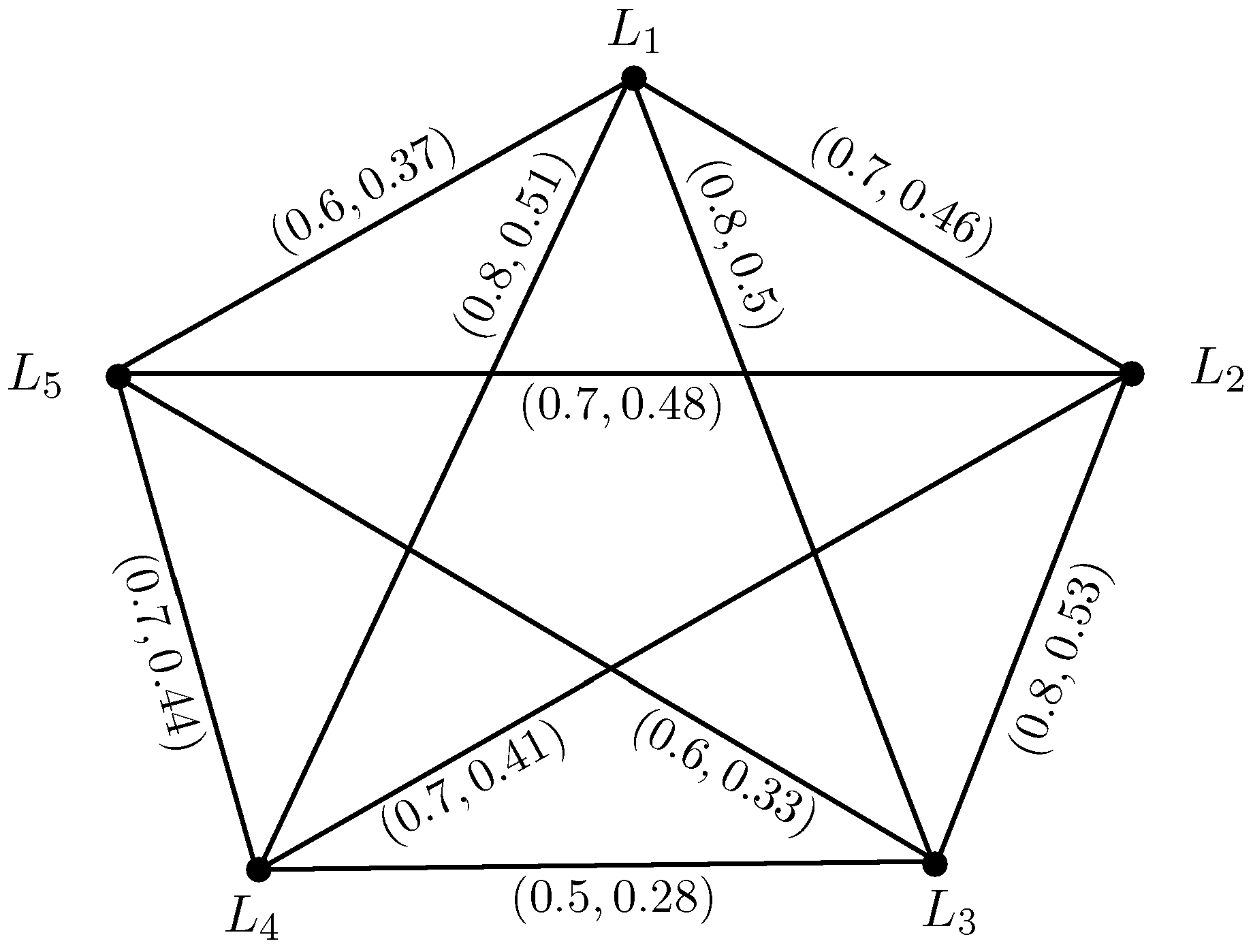
Here we explain the use of mF matroids in network analysis. The 2-polar fuzzy graph in Figure 2 represents the wireless communication between five locations .
The degree of membership of each edge shows the time taken and cost for sending a message from one location to the other. Each pair of vertices is connected by an edge. However, in general we do not need connections among all the vertices because the vertices linked indirectly will also have a message service between them, i.e., if there is a connection from to and to , then we can send a message from to , even if there is no edge between and . The problem is to find a set of edges such that we are able to send message between every two vertices under the condition that time and cost is minimum. The procedure is as follows. Arrange the membership values of edges in increasing order as, , , , , , , , , , . At each step, select an edge having minimum membership value so that it does not create any circuit with previous selected edges. The -polar fuzzy set of selected edges is,
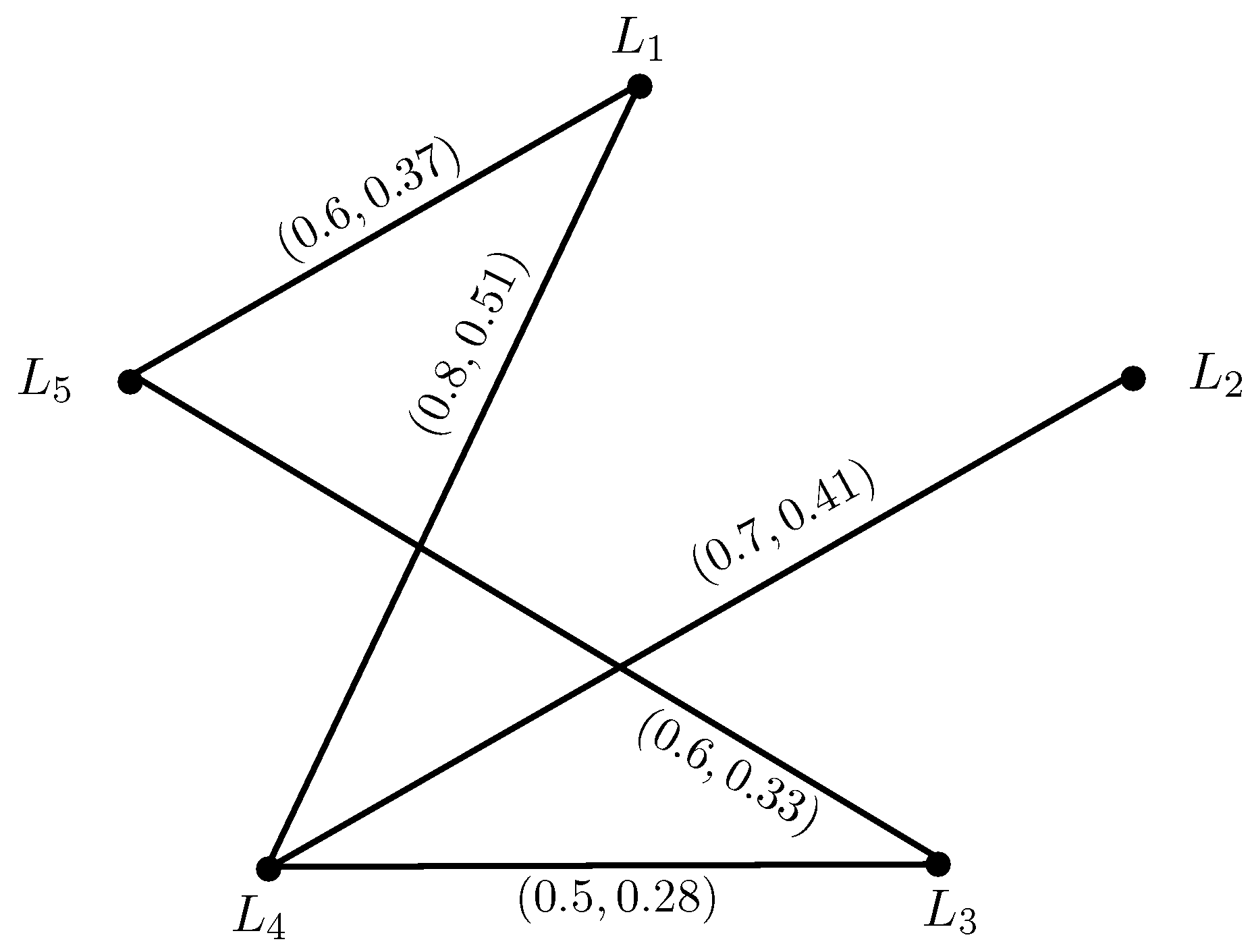
The communication network with minimum number of locations and cost is shown in Figure 3.
Figure 3 shows that only five connections are needed to communicate among given locations in order to minimize the cost and improve the network communication.
5. Conclusions
In this research paper, we have applied the powerful technique of mF sets to extend the theory of vector spaces and matroids. The mF models give more accuracy, precision and compatibility to the system when more than one agreements are to be dealt with. We have mainly introduced the idea of the mF matroid, implemented this concept to graph theory, linear algebra and have studied various examples including the mF uniform matroid, mF linear matroid, mF partition matroid and mF cycle matroid. We have also presented the idea of mF circuit, closure of mF matroid and put special emphasis on mF rank function. The paper is concluded with some real life applications of mF matroids in decision support system, ordering of machines to perform specific tasks and detection of minimum number of locations in wireless network in order to motivate the idea presented in this research paper. We are extending our work to (1) decision support systems based on intuitionistic fuzzy soft circuits, (2) fuzzy rough soft circuits, (3) and neutrosophic soft circuits.
Author Contributions
Musavarah Sarwar and Muhammad Akram conceived of the presented idea. Musavarah Sarwar developed the theory and performed the computations. Muhammad Akram verified the analytical methods.
Conflicts of Interest
The authors declare no conflict of interest.
References
- Whitney, H. On the abstract properties of linear dependence. Am. J. Math. 1935, 57, 509–533. [Google Scholar] [CrossRef]
- Zadeh, L.A. Fuzzy sets. Inf. Control 1965, 8, 338–353. [Google Scholar] [CrossRef]
- Zadeh, L.A. Similarity relations and fuzzy orderings. Inf. Sci. 1971, 3, 177–200. [Google Scholar] [CrossRef]
- Petković, D.; Gocić, M.; Shamshirband, S. Adaptive neuro-fuzzy computing technique for precipitation estimation. Facta Univ. Ser. Mech. Eng. 2016, 14, 209–218. [Google Scholar]
- Ćirović, G.; Pamučar, D. Decision support model for prioritizing railway level crossings for safety improvements. Expert Syst. Appl. 2013, 91, 89–106. [Google Scholar]
- Radu-Emil, P.; Stefan, P.; Claudia-Adina, B.-D. Automotive applications of evolving Takagi-Sugeno-Kang fuzzy models. Facta Univ. Ser. Mech. Eng. 2017, 15, 231–244. [Google Scholar]
- Lukovac, V.; Pamučar, D.; Popović, M.; Đorović, B. Portfolio model for analyzing human resources: An approach based on neuro-fuzzy modeling and the simulated annealing algorithm. Expert Syst. Appl. 2017, 90, 318–331. [Google Scholar] [CrossRef]
- Pamučar, D.; Petrović, I.; Ćirović, G. Modification of the BestWorst and MABAC methods: A novel approach based on interval-valued fuzzy-rough numbers. Expert Syst. Appl. 2018, 91, 89–106. [Google Scholar]
- Zhang, W.-R. Bipolar fuzzy sets and relations: A computational framework for cognitive modeling and multiagent decision analysis. In Proceedings of the IEEE Conference Fuzzy Information Processing Society Biannual Conference, San Antonio, TX, USA, 18–21 December 1994; pp. 305–309. [Google Scholar]
- Akram, M.; Feng, F.; Borumand Saeid, A.; Fotea, V. A new multiple criteria decision-making method based on bipolar fuzzy soft graphs. Iran. J. Fuzzy Syst. 2017. [Google Scholar] [CrossRef]
- Sarwar, M.; Akram, M. Novel concepts bipolar fuzzy competition graphs. J. Appl. Math. Comput. 2016, 54, 511–547. [Google Scholar] [CrossRef]
- Sarwar, M.; Akram, M. Certain algorithms for computing strength of competition in bipolar fuzzy graphs. Int. J. Uncertain. Fuzziness Knowl. Based Syst. 2017, 25, 877–896. [Google Scholar] [CrossRef]
- Chen, J.; Li, S.; Ma, S.; Wang, X. m-polar fuzzy sets: An extension of bipolar fuzzy sets. Sci. World J. 2014, 416530. [Google Scholar] [CrossRef] [PubMed]
- Akram, M.; Younas, H.R. Certain types of irregular m-polar fuzzy graphs. J. Appl. Math. Comput. 2017, 53, 365–382. [Google Scholar] [CrossRef]
- Akram, M.; Sarwar, M. Novel applications of m-polar fuzzy hypergraphs. J. Intell. Fuzzy Syst. 2017, 32, 2747–2762. [Google Scholar] [CrossRef]
- Sarwar, M.; Akram, M. Novel applications of m-polar fuzzy concept lattice. New Math. Nat. Comput. 2017, 13, 261–287. [Google Scholar] [CrossRef]
- Akram, M.; Sarwar, M. Transversals of m-polar fuzzy hypergraphs with applications. J. Intell. Fuzzy Syst. 2016, 32, 351–364. [Google Scholar] [CrossRef]
- Akram, M.; Sarwar, M. Novel applications of m-polar fuzzy competition graphs in decision support system. Neural Comput. Appl. 2017. [Google Scholar] [CrossRef]
- Goetschel, R.; Voxman, W. Fuzzy matroids. Fuzzy Sets Syst. 1988, 27, 291–302. [Google Scholar] [CrossRef]
- Goetschel, R.; Voxman, W. Bases of fuzzy matroids. Fuzzy Sets Syst. 1989, 31, 253–261. [Google Scholar] [CrossRef]
- Sarwar, M.; Akram, M. Representation of graphs using m-polar fuzzy environment. Ital. J. Pure Appl. Math. 2017, 38, 291–312. [Google Scholar]
- Akram, M.; Waseem, N. Certain metric in m-polar fuzzy graphs. New Math. Nat. Comput. 2016, 12, 135–155. [Google Scholar] [CrossRef]
- Li, S.; Yang, X.; Li, H.; Ma, M. Operations and decompositions of m-polar fuzzy graphs. Basic Sci. J. Text. Univ./Fangzhi Gaoxiao Jichu Kexue Xuebao 2017, 30, 149–162. [Google Scholar]
- Hsueh, Y.-C. On fuzzification of matroids. Fuzzy Sets Syst. 1993, 53, 319–327. [Google Scholar] [CrossRef]
- Akram, M.; Adeel, A. m-polar fuzzy labeling graphs with application. Math. Comput. Sci. 2016, 10, 387–402. [Google Scholar] [CrossRef]
- Akram, M.; Akmal, R. Certain concepts in m-polar fuzzy graph structures. Discret. Dyn. Nat. Soc. 2016, 2016, 6301693. [Google Scholar] [CrossRef]
- Akram, M.; Waseem, N.; Dudek, W.A. Certain types of edge m-polar fuzzy graphs. Iran. J. Fuzzy Syst. 2017, 14, 27–50. [Google Scholar]
- Koczy, K.T. Fuzzy graphs in the evaluation and optimization of networks. Fuzzy Sets Syst. 1992, 46, 307–319. [Google Scholar] [CrossRef]
- Mathew, S.; Sunitha, M.S. Types of arcs in a fuzzy graph. Inf. Sci. 2009, 179, 1760–1768. [Google Scholar] [CrossRef]
- Novak, L.A. A comment om “Bases of fuzzy matroids”. Fuzzy Sets Syst. 1997, 87, 251–252. [Google Scholar] [CrossRef]
- Sarwar, M.; Akram, M. An algorithm for computing certain metrics in intuitionistic fuzzy graphs. J. Intell. Fuzzy Syst. 2016, 30, 2405–2416. [Google Scholar] [CrossRef]
- Wilson, R.J. An Introduction to matroid theory. Am. Math. Mon. 1973, 80, 500–525. [Google Scholar] [CrossRef]
- Zafar, F.; Akram, M. A novel decision making method based on rough fuzzy information. Int. J. Fuzzy Syst. 2017. [Google Scholar] [CrossRef]
- Mordeson, J.N.; Nair, P.S. Fuzzy Graphs and Fuzzy Hypergraphs, 2nd ed.; Physica Verlag: Heidelberg, Germany, 2001. [Google Scholar]
Figure 1.
3-polar fuzzy multigraph.
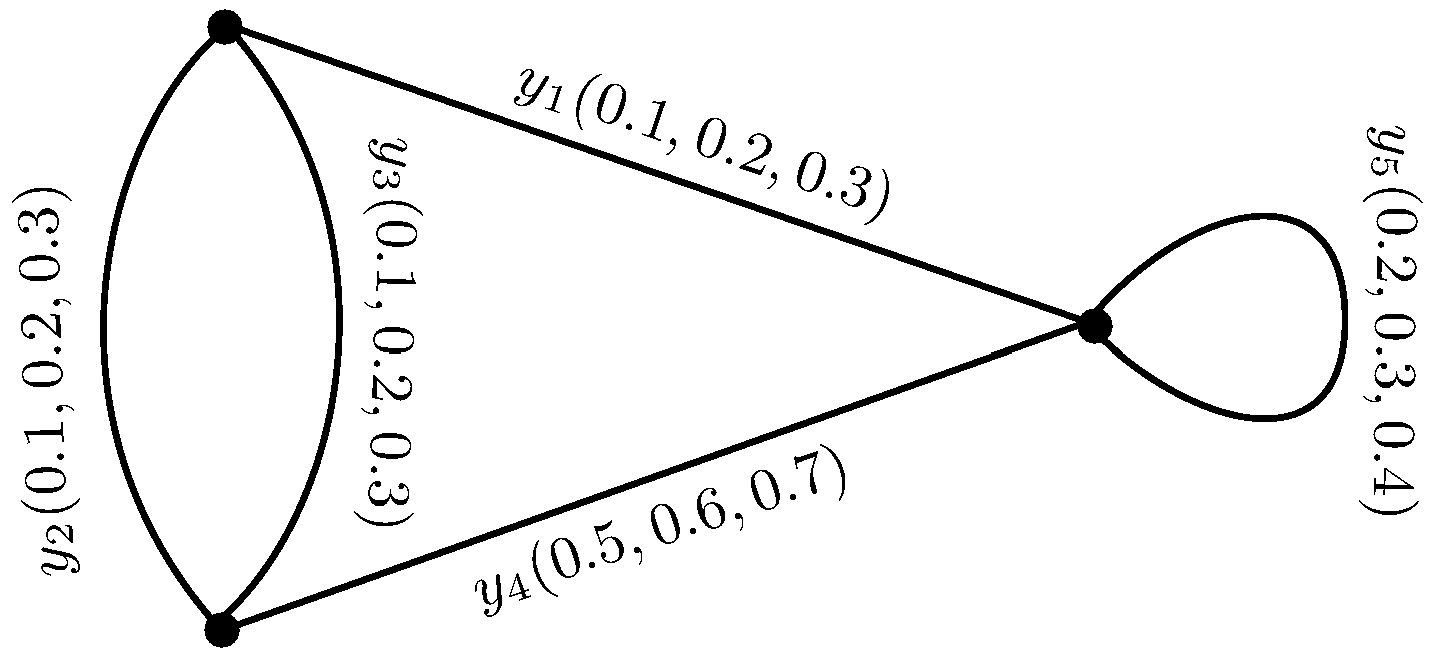
Figure 2.
Wireless communication.

Figure 3.
Communication network with minimum connections.

© 2017 by the authors. Licensee MDPI, Basel, Switzerland. This article is an open access article distributed under the terms and conditions of the Creative Commons Attribution (CC BY) license (http://creativecommons.org/licenses/by/4.0/).
Share and Cite
MDPI and ACS Style
Sarwar, M.; Akram, M. New Applications of m-Polar Fuzzy Matroids. Symmetry 2017, 9, 319. https://doi.org/10.3390/sym9120319
AMA Style
Sarwar M, Akram M. New Applications of m-Polar Fuzzy Matroids. Symmetry. 2017; 9(12):319. https://doi.org/10.3390/sym9120319
Chicago/Turabian StyleSarwar, Musavarah, and Muhammad Akram. 2017. "New Applications of m-Polar Fuzzy Matroids" Symmetry 9, no. 12: 319. https://doi.org/10.3390/sym9120319
Note that from the first issue of 2016, this journal uses article numbers instead of page numbers. See further details here.