
Aesthetic Patterns with Symmetries of the Regular Polyhedron

1
School of Mathematics & Physics, Jinggangshan University, Ji’an 343009, China
2
School of Water Conservancy and Electric Power, Hebei University of Engineering, Handan 056021, China
*
Author to whom correspondence should be addressed.
Symmetry 2017, 9(2), 21; https://doi.org/10.3390/sym9020021
Submission received: 14 December 2016
/
Revised: 18 January 2017
/
Accepted: 22 January 2017
/
Published: 3 February 2017
(This article belongs to the Special Issue Polyhedral Structures)
Abstract
:A fast algorithm is established to transform points of the unit sphere into fundamental region symmetrically. With the resulting algorithm, a flexible form of invariant mappings is achieved to generate aesthetic patterns with symmetries of the regular polyhedra.
1. Introduction
Due to the perfect symmetry of regular polyhedra, they have been the subject of wide attention [1,2,3,4,5,6]. Dutch artist Escher et al. [7] designed several amazing woodcarvings of polyhedral symmetries. His artwork inspired Séquin and Yen to design and manufacture similar spherical artwork semiautomatically [8]. With the development of modern computers, there is considerable research on the automatic generation of aesthetic patterns; see the doctoral dissertation of Kaplan [9] and references therein. Such patterns simultaneously possess complex form and harmonious geometry structure, which exhibit the beauty of math. In this paper, we first review the merit and drawback of strategies used in creating symmetrical patterns. Then, we present a new approach to yield aesthetic patterns with symmetries of the regular polyhedra.
Let and be, respectively, a symmetry group and a mapping. is called invariant with respect to if it satisfies:
is called equivariant with respect to if it satisfies:
Invariant mapping and equivariant mapping are two important methods adopted to generate symmetrical patterns. Mathematicians have highlighted the importance of such mappings in many situations [10,11]. Field and Golubitsky first proposed equivariant mappings to yield aesthetic patterns with discrete planar symmetries [12]. This idea later inspired Reiter to create chaotic attractors with symmetries of the tetrahedron [13] and octahedron [14] in three-dimensional Euclidean space . Recently, Lu et al. established several families of invariant mappings to generate similar images [15]. All the mappings used above are polynomials, because invariant or equivariant mappings of the polynomial form are easier to construct. However, polynomials are not appropriate to create visually appealing patterns, since they lack variety. Furthermore, for the symmetry group of complex generators, even polynomials are not easy to construct. This is why polynomials do not appear to yield regular dodecahedron patterns of great complexity. Group summation is a classic technique used in the invariant theory [16]. To generate patterns with symmetries of the regular polyhedra, Chung introduced this technique and constructed a flexible form of equivariant mappings [17]. However, this kind of mapping still has to meet certain requirements. The general summation form of equivariant mappings:
was proposed by Dumont, where f is a mapping from to , G is a finite group, and the order of G [18]. They utilized (3) to explore chaotic attractors with symmetries that are close to forbidden symmetries. Since f in (3) can be arbitrary mappings rather than the particular polynomials, one can choose f freely, and the resulting patterns are more beautiful. Following (3), Jones et al. created many appealing attractors [19]; Reiter successfully realized a dodecahedron attractor that possesses complex symmetries [20]. Dumont later improved (3) so that it could be applicable for crystallographic point groups [21].
Although (3) is easy to construct and theoretically feasible for any finite group, this strategy is not appropriate for the symmetry group of large order. Notice that there are terms in the summation; for a group of large order, (3) usually has ill-conditioned sensitivity. This leads to patterns that have unaesthetic noise. For example, regular dodecahedron attractors of 120 symmetries generated by (3) [20] are not as beautiful as images shown in [19]. Computational cost is also a problem of (3) that should not be neglected. Dumont experimented with space group 227 of order 192 [21]. They commented that “finding a visually interesting attractor for this group was most challenging because experiments ran slowly”.
Regular polytopes are higher-dimensional generalizations of regular polyhedra. Their structures are similar to that of regular polyhedra, but with more symmetries. For example, symmetries of 24-cell and 600-cell in are 1152 and 14,400, respectively, which far exceed the symmetries of any regular polyhedron [22]. In this paper, we present a fast and convenient approach to generating aesthetic patterns with symmetries of the regular polyhedra. The proposed mapping not only has flexible form, but also avoids the order restriction appearing in (3).
2. Symmetry Groups of Regular Polyhedra
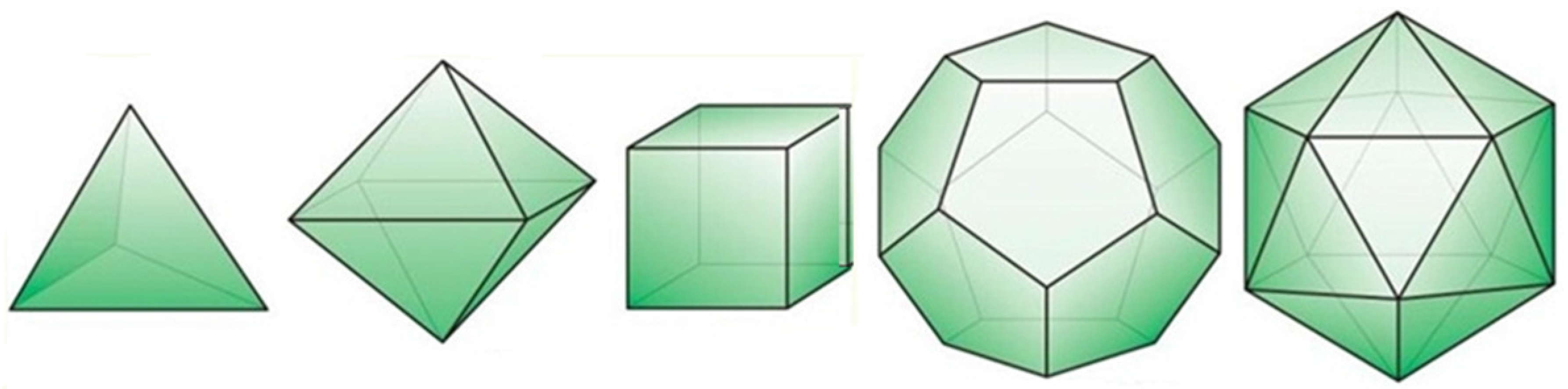
A regular polyhedron is a convex polyhedron whose faces are regular and equal and whose vertices have similar neighborhoods. A regular polyhedron can be briefly represented as Schläfli symbol of the form , where p is the number of sides of each face and q the number of faces meeting at each vertex [1]. There are five regular polyhedra, better known as Platonic solids: tetrahedron , octahedron , cube , dodecahedron , and icosahedron (Figure 1).
Groups generated by reflections deserve special consideration for two reasons: (1) there is a general theory covering them all; (2) they contain the remaining point groups as subgroups [1,22]. This section concerns the reflection groups of regular polyhedra. For convenience, we denote the reflection group of as . We first introduce some basic concepts.
Given an object , a symmetry of is a congruent or isometric transformation. The symmetry group of comprises all its symmetries. The elements , , ... of group are called a set of generators if every element of is expressible as a finite product of their powers (including negative powers). The fundamental region under group is a connected set whose transformed copies under the action of cover the entire space without overlapping, except at boundaries. In Euclidean space, a reflection group is a discrete group which is generated by a set of reflections.
Suppose that and are generators of . Then:
is an abstract presentation of , where I is the identity [22]. Since and are dual, they share the same symmetry group .
Let be a regular polyhedron inscribed in the unit sphere . By joining the center O of and a point A of , the directed line intersects at a point . For a given , this projection establishes an equivalence relation between regular polyhedron and spherical tiling projected on . Therefore, spherical tiling can be indiscriminately regarded as . Henceforth, we concentrate on spherical tiling instead of regular polyhedron itself.
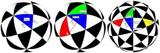
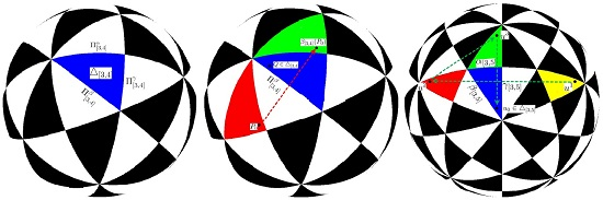
Geometrically, generators and are reflections which can be realized as orthogonal matrixes. Let and be, respectively, reflection planes associated with and . Then, the region surrounded by those planes forms a spherical right triangle on . Repeated reflections along sides of will tile exactly once. This suggests that is a fundamental region associated with . Figure 2a illustrates a fundamental region .
Generators , and , and fundamental region are important contents of the next section. We summarize them as follows and refer the reader to [17] for more details.
- ■
- Tetrahedral group :
- ■
- Octhedral group :
- ■
- Icosahedral group :
3. Transform Points of into Fundamental Region Symmetrically
In this section, we present a fast algorithm that transforms points of into fundamental region symmetrically. To this end, we first prove a lemma.
Lemma 1.
Let be a plane in with ,
be the reflection R associated with Π. Assume and are points on the different sides of Π; i.e.:
Then:
where norm represents spherical distance.
Proof.
By the formula of spherical distance, Assume then direct computation shows So the spherical distance between and is:
We use a diagram to explain the geometric meaning of Lemma 1. In Figure 2b, let and be points on the different sides of plane . Then, and Q lie on the same side of . Lemma 1 says that the distance between and Q is smaller than and Q. In other words, for two points on the different sides of a plane, reflection transformation of the plane can shorten their distance.
Theorem 1.
Let be the fundamental region with respect to , Q be an interior point of . For a point outside , the following algorithm determines a transformation and a symmetrically placed point so that .
Step 1: let , .
Step 2: compute , where
Step 3: choose so that is the subscript of ,
Step 4: let , .
Step 5: if , stop; otherwise, set , repeat Steps 2–5.
Step 6: assume n is the number of cycles, then , where:
Proof.
, , and are isometrical symmetrical transformations, so obtained in Step 4 is always a symmetrical point of lying on . Recall that fundamental region is a spherical triangle surrounded by planes , , and . For , there must exist a plane , so that and Q lie on different sides of Π. By Lemma 1, there exists a reflection associated with Π so that:
Thus, each time a chosen transformation is employed, the transformed will get nearer to Q, and eventually fall into . Let , then . ☐
Theorem 1 describes an algorithm that transforms points of into symmetrically. Figure 2c illustrates an example of how Theorem 1 works.
By the definition of fundamental region, copies of can tile exactly once; i.e.,
where is the order of group . Indeed, for , Theorem 1 provides a method to find a specific of the form (17) so that . Thus, we can use Theorem 1 to determine entire elements of automatically. In practice, we found that the algorithm of Theorem 1 is a very fast algorithm. On average, each point of will be transformed into , , within 3.16, 4.70, 7.94 times. Essentially, regular polytopes and polyhedra have the same kind of symmetry groups—finite reflection groups. This means that it should be possible to extend this fast algorithm to treat regular polytopes with thousands of symmetries.
4. Colorful Spherical Patterns with Symmetry
In this section, we describe how to create colorful spherical patterns with symmetry.
For a point , we define a mapping of the form:
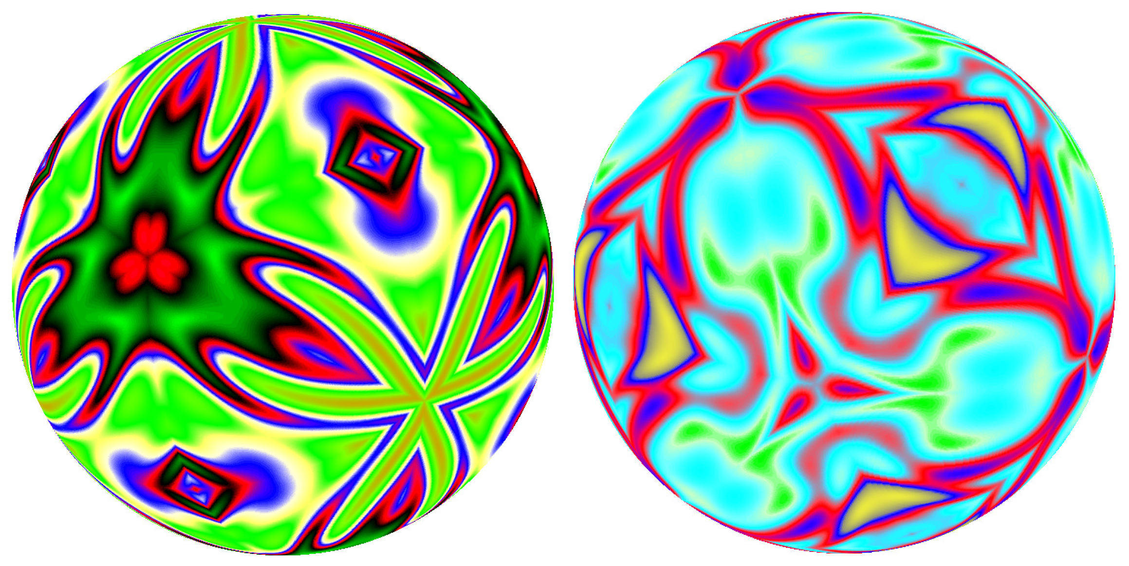
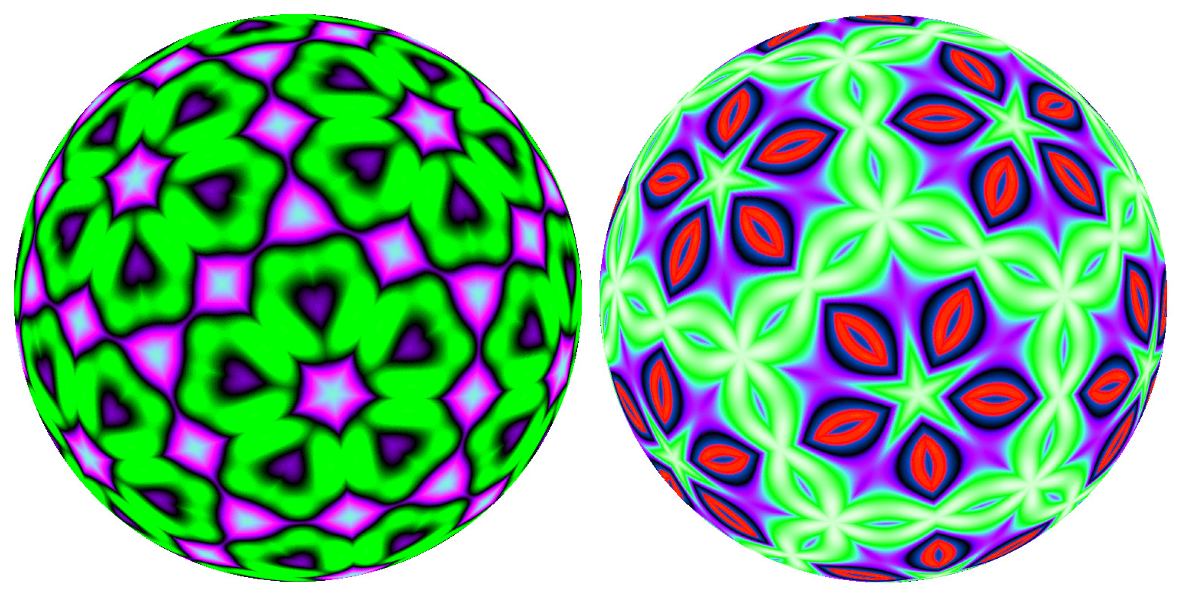
where is a transformation determined by Theorem 1, is an arbitrary mapping from to . By (1), mapping is essentially an invariant mapping associated with . Let be the the kth iteration of at . For a given positive integer m, by the dynamical behavior of iteration sequences , we assign a certain color to . Using this method, point and its symmetrical point () will be assigned the same color. Consequently, the colored obtained by this method will have symmetries. Figure 2, Figure 3, Figure 4 and Figure 5 show six aesthetic patterns obtained in this manner.
The color scheme used above was borrowed from [23]. We have employed this scheme to render fractal [24] and hyperbolic patterns [25], which could enhance the visual appeal of patterns effectively. We refer the reader to [26] for more details.
Equation (19) has the following outstanding features. First, to create symmetrical patterns, one needs to construct mappings that meet certain requirements [12,13,14,15,17,18,19,20,21]. However, under certain circumstances, this kind of mapping is not easy to achieve. Mapping (19) has no requirements, and we can construct mappings at will. For example, the mapping used in the left of Figure 3 is:
Acknowledgments
We produced Figure 2, Figure 3, Figure 4 and Figure 5 in the VC++ 6.0 programming environment with the aid of OpenGL, a powerful graphics software package. We thank Adobe and Microsoft for their friendly technical support. This work was supported by the Natural Science Foundation of China (No. 11461035) and Doctoral Startup Fund of Jingangshan University (Nos. JZB1303, JZB11002).
Author Contributions
Peichang Ouyang conceived the framework and structured the whole paper; Liying Wang performed the experiments and wrote the paper; Tao Yu and Xuan Huang checked the results; Peichang Ouyang, Liying Wang, Tao Yu and Xuan Huang completed the revision of the article.
Conflicts of Interest
The authors declare no conflict of interest.
References
- Coxeter, H.S.M. Regular Polytopes; Dover: New York, NY, USA, 1973. [Google Scholar]
- Mcmulle, P.; Schulte, E. Abstract Regular Polytopes; Cambridge University Press: Cambridge, UK, 2002. [Google Scholar]
- Conway, J.H.; Burgiel, H.; Goodman-Strauss, C. The Symmetries of Things; A K Peters Press: Natick, MA, USA, 2008. [Google Scholar]
- Armstrong, V.E. Groups and Symmetry; Springer: New York, NY, USA, 1987. [Google Scholar]
- Magnus, W. Noeuclidean Tessellation and Their Groups; Academic Press: New York, NY. USA, 1974. [Google Scholar]
- Rees, E.G. Notes on Geometry; Springer: Berlin/Heidelberg, Germany, 1983. [Google Scholar]
- Escher, M.C.; Ford, K.; Vermeulen, J.W. Escher on Escher: Exploring the Infinity; Harry N. Abrams: New York, NY, USA, 1989. [Google Scholar]
- Yen, J.; Séquin, C. Escher Sphere Construction Kit. In Proceedings of the 2001 Symposium on Interactive 3D Graphics, Research Triangle Park, NC, USA, 19–21 March 2001; pp. 95–98.
- Kaplan, C.S. Computer Graphics and Geometric Ornamental Design. Ph.D. Thesis, University of Washington, Washington, DC, USA, 2002. [Google Scholar]
- Field, M. Dynamics and Symmetry; Imperial College Press: London, UK, 2007. [Google Scholar]
- Humphreys, J.E.; Bollobas, B.; Fulton, W.; Katok, A.; Kirwan, F.; Sarnak, P.; Simon, B. Reflection Groups and Coxeter Groups; Cambridge University Press: Cambridge, UK, 1992. [Google Scholar]
- Field, M.; Golubitsky, M. Symmetry in Chaos; Oxford University Press: Oxford, UK, 1992. [Google Scholar]
- Reiter, C.A. Chaotic Attractors with the Symmetry of the Tetrahedron. Comput. Graph. 1997, 6, 841–884. [Google Scholar] [CrossRef]
- Brisson, G.F.; Gartz, K.M.; McCune, B.J.; O’Brien, K.P.; Reiter, C.A. Symmetric Attractors in Three-dimensional Space. Chaos Soliton Fract. 1996, 7, 1033–1051. [Google Scholar] [CrossRef]
- Lu, J.; Zou, Y.R.; Liu, Z.Y. Colorful Symmetric Images in Three-dimensional Space from Dynamical Systems. Fractals 2012, 20, 53–60. [Google Scholar] [CrossRef]
- Benson, D.J.; Hitchin, N.J. Polynomial Invariant of Finite Groups; Cambridge University Press: Cambridge, UK, 1993. [Google Scholar]
- Chung, K.W.; Chan, H.S.Y. Spherical Symmetries from Dynamics. Comput. Math. Appl. 1995, 7, 67–81. [Google Scholar] [CrossRef]
- Dumont, J.P.; Reiter, C.A. Chaotic Attractors Near Forbidden Symmetry. Chaos Soliton Fract. 2000, 11, 1287–1296. [Google Scholar] [CrossRef]
- Jones, K.C.; Reiter, C.A. Chaotic Attractors with Cyclic Symmetry Revisited. Comput. Graph. 2000, 24, 271–282. [Google Scholar] [CrossRef]
- Reiter, C.A. Chaotic Attractors with the Symmetry of the Dodecahedron. Vis. Comput. 1999, 4, 211–215. [Google Scholar] [CrossRef]
- Dumont, J.P.; Heiss, F.J.; Jones, K.C.; Reiter, C.A.; Vislocky, L.M. N-dimensional Chaotic Sttractors with Crystallographic Symmetry. Chaos Soliton Fract. 2001, 4, 761–784. [Google Scholar] [CrossRef]
- Coxeter, H.S.M.; Moser, W.O.J. Generators and Relations for Discrete Groups; Springer: New York, NY, USA, 1980. [Google Scholar]
- Lu, J.; Ye, Z.X.; Zou, Y.R. Colorful Patterns with Discrete Planar Symmetries from Dynamical Systems. Fractals 2012, 18, 35–43. [Google Scholar] [CrossRef]
- Ouyang, P.C.; Fathauer, R.W. Beautiful Math, Part 2, Aesthetic Patterns Based on Fractal Tilings. IEEE Comput. Graph. 2014, 1, 68–75. [Google Scholar] [CrossRef] [PubMed]
- Ouyang, P.C.; Chung, K.W. Beautiful Math, Part 3, Hyperbolic Aesthetic Patterns Based on Conformal Mappings. IEEE Comput. Graph. 2014, 2, 72–79. [Google Scholar] [CrossRef] [PubMed]
- Ouyang, P.C.; Cheng, D.S.; Cao, Y.H.; Zhan, X.G. The Visualization of Hyperbolic Patterns from Invariant Mapping Method. Comput. Graph. 2012, 2, 92–100. [Google Scholar] [CrossRef]
Figure 1.
The five regular polyhedra.

Figure 2.
(a) The blue spherical right triangle surrounded by planes , and forms a fundamental region associated with group ; (b) Let and be two points on the different sides of . Then, and Q lie on the same side of , and the distance between them is smaller than and Q; and (c) A schematic illustration that shows how Theorem 1 transforms into symmetrically. In this case, is first transformed by so that goes into red tile. Then, is transformed by so that goes into green tile. At last, is transformed by so that .
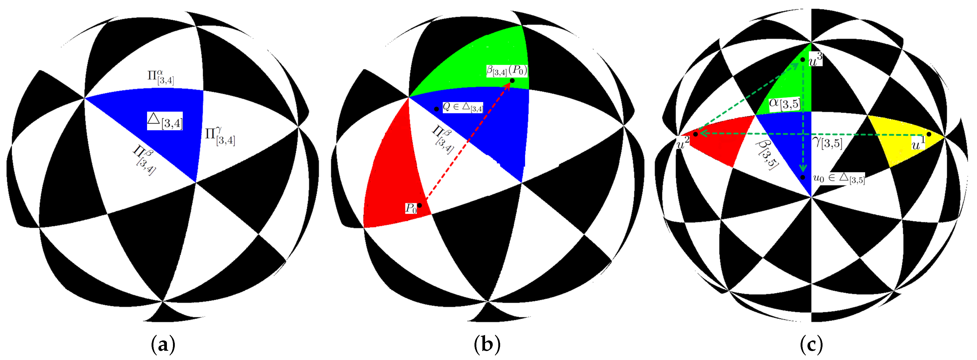
Figure 3.
Two spherical patterns with [3,3] symmetries.

Figure 4.
Two spherical patterns with [3,4] symmetries.
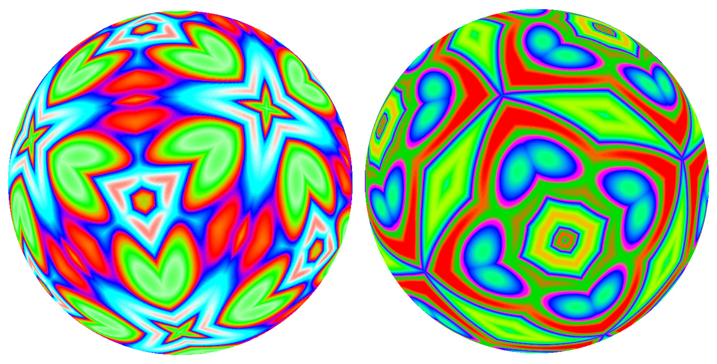
Figure 5.
Two spherical patterns with [3,5] symmetries.

© 2017 by the authors. Licensee MDPI, Basel, Switzerland. This article is an open access article distributed under the terms and conditions of the Creative Commons Attribution (CC BY) license ( http://creativecommons.org/licenses/by/4.0/).
Share and Cite
MDPI and ACS Style
Ouyang, P.; Wang, L.; Yu, T.; Huang, X. Aesthetic Patterns with Symmetries of the Regular Polyhedron. Symmetry 2017, 9, 21. https://doi.org/10.3390/sym9020021
AMA Style
Ouyang P, Wang L, Yu T, Huang X. Aesthetic Patterns with Symmetries of the Regular Polyhedron. Symmetry. 2017; 9(2):21. https://doi.org/10.3390/sym9020021
Chicago/Turabian StyleOuyang, Peichang, Liying Wang, Tao Yu, and Xuan Huang. 2017. "Aesthetic Patterns with Symmetries of the Regular Polyhedron" Symmetry 9, no. 2: 21. https://doi.org/10.3390/sym9020021
Note that from the first issue of 2016, this journal uses article numbers instead of page numbers. See further details here.