A Symmetry Particle Method towards Implicit Non‐Newtonian Fluids

University of Science and Technology Beijing, Xueyuan Road 30, Haidian District, Beijing, China, 100083
*
Author to whom correspondence should be addressed.
Symmetry 2017, 9(2), 26; https://doi.org/10.3390/sym9020026
Submission received: 17 January 2017
/
Accepted: 10 February 2017
/
Published: 17 February 2017
(This article belongs to the Special Issue Symmetry in Cooperative Applications II)
Abstract
:In this paper, a symmetry particle method, the smoothed particle hydrodynamics (SPHs) method, is extended to deal with non-Newtonian fluids. First, the viscous liquid is modeled by a non-Newtonian fluid flow and the variable viscosity under shear stress is determined by the Carreau-Yasuda model. Then a pressure correction method is proposed, by correcting density error with individual stiffness parameters for each particle, to ensure the incompressibility of fluid. Finally, an implicit method is used to improve efficiency and stability. It is found that the non-Newtonian behavior can be well displayed in all cases, and the proposed SPH algorithm is stable and efficient.
1. Introduction
Non-Newtonian fluid is widely presented in industry, mining engineering, food processing, and many other fields in cases such as pit filled paste, blood, honey, etc. However, the physical nature of non-Newtonian fluid is very complicated. It is pretty difficult to exactly simulate non-Newtonian fluid. A non-Newtonian fluid has characteristic properties of both solids and fluids [1]. Take the shear thinning non-Newtonian fluid for example, when it flows with low velocity, its viscosity becomes higher, and the fluid starts to exhibit properties of solids; while as it flows with high velocity, its viscosity gets smaller, and the non-Newtonian fluid exhibits liquid properties. In recent years, smoothed particle hydrodynamics (SPHs) [2] has become an important Lagrangian method for industrial flow simulation [3] and computational fluid dynamics [4,5]. Because of the symmetry of SPH method with respect to translations, rotations, and time, the exact conservation of momentum, angular momentum and energy are guaranteed [6,7,8,9]. There are several difficulties to simulating non-Newtonian fluids. Firstly, how to model the non-Newtonian fluid. Due to the non-linear relationship between viscosity and shear force, the adequate physical equations and stable approximate simulation method should be re-established for non-Newtonian fluids. Secondly, how to ensure the incompressibility of non-Newtonian fluids. SPH method has some inherent problems which are the same as massless methods [10]. Enforcing incompressibility for particle methods is a challenging problem [11]. Thirdly, how to improve the efficiency of simulation. Due to the complicated physical equations of non-Newtonian fluids, a small time step is necessary, which proves to be rather time-consuming.
A novel non-Newtonian fluid simulation method for SPH is proposed in this article. The viscous liquid is modeled by a non-Newtonian fluid flow, and the variable viscosity under shear stress is achieved using a viscosity model known as the Carreau-Yasuda model. To improve numerical stability, a pressure correction method is used to correct density error by setting up individual stiffness parameters for each particle. Furthermore, an implicit viscosity solver is proposed for non-Newtonian SPH fluid.
2. Related Works
There are two major approaches to simulate non-Newtonian fluid: Eulerian method and Lagrangian method. The Lagrangian method treats fluid as a particle system. Each point in the fluid is labeled as a separate particle, with a position and a velocity. Instead of tracking each particle, the Eulerian method can look at fixed points in space and see how the fluid quantities (such as density, velocity, etc.) measured at those points change in time [12].
For the Eulerian method, the main problems are how to model non-Newtonian fluid and how to deal with free surface. Goatskin et al. [13] proposed a quasi-linear plastic model to control the change of viscosity in the gradual transformation from a solid to a non-Newtonian fluid. This model meets the von Mises’s yield condition. They simulated the melting of a piece of wax with this model by using explicit Euler method. Losasso et al. [14] modeled unified fluids with different viscoelasticities and densities by extending the particle level set. There are many different level sets in the same grid region. The exchanges between different level sets can be achieved by adding the pressure correction process before calculating viscosity. Batty and Bridson [15] found out that the Laplace operator and Strain rate items of non-Newtonian fluid should be computed under the velocity field with no divergence; therefore, the pressure correction process was added after the calculation of viscosity. Besides, they proposed an implied unconditionally stable simulation method based on marker-and-cell. Even though they proposed high precision free surface boundary conditions, it still cannot simulate high viscosity Newtonian fluid. Bergou et al. [16] proposed a method based on discrete differential geometry to simulate one dimensional linear viscous fluid. This approach can simulate one dimensional phenomenon vividly, but distortion often appeared when the flow layer got thicker. Batty and Uribe [17] simulated thin viscous layer with dimensionality deduce technology. They combined nonlinear surface tension and smallest-discrete-surface-area-based formulas and reserved the mass of unit triangular mesh with the local grid reconstruction technology. This approach can simulate the physical conditions of viscous thin layer, such as bending and draping.
Particle-based methods are superior when free surface and complex interface are to be dealt with. So mesh free methods represented by SPH method have been more commonly applied in the field of non-Newtonian fluid simulation [18,19]. Müller et al. [20] simulated fluids of high elasticity and high plasticity by structuring a point-based animation modeling method. He combined continuum mechanics with von Mises’ yield condition and calculated the displacement and the velocity using moving least squares. Afonso et al. [21] also completed simulations with a General Newtonian Fluid model, and the viscosity of fluid was controlled by the Jump Number. The melting process of a heated non-Newtonian fluid [22], which later becomes a low viscosity fluid, was also modeled by the general Newtonian fluid model. Rafiee et al. [23] proposed a free surface SPH method. This method can be applied to Newton fluid and viscoplastic fluid, and simulate the bending phenomena of viscous fluids. The relationship between the pressure and the viscosity of non-Newtonian fluids was described with the real polymer state equation [24]. Andrade et al. [25] can simulate the flow of polymer with high viscosity and high pressure. In addition, the unified molding of viscous Newtonian fluid and shear thinning non-Newtonian fluid were simulated, but this method can only simulate fluid with low viscosity; whereas unstable phenomenon would appear when the time step is larger. Zhang et al. [26] proposed an explicit method for shear thinning non-Newtonian fluid.
In addition to Euler and Lagrange methods, recently there is a novel alternative, the codimensional method [27], which is able to simulate a non-Newtonian fluid. This method enables the simulation of interaction between different dimensions of a non-Newtonian fluid, such as filamentous remaining marks left on a pool of paint after getting brushed over, which is difficult for Euler and Lagrange methods to achieve.
For Newtonian fluid simulation, the standard SPH has been gradually replaced by a predictive–corrective method to ensure incompressibility with larger time step. Predictive–corrective algorithm was first proposed by Solenthaler and Pajarola [28], which is to predict the state of a fluid in absence of pressure, then use pressure for its conduct correction. Ihmsen et al. [29] proposed an implicit SPH method that adjusts fluid’s density by pressure according to the relationship between density and velocity in the next time step. Bender and Koschier [30] proposed a divergence-free velocity method, which is essentially also a predictive–corrective method that prevents volume compression and enforces a divergence-free velocity field formulation of the physical laws. However, none of them involved non-Newtonian fluid simulation.
3. Material Model
3.1. Governing Equations
In the SPH scheme, the fluid is described as moving particles with physical attributes such as position , velocity , and mass . Mass is used to determine the local geometry of the fluid and assumed to be constant. Non-Newtonian fluids are a continuous medium whose motion equations must follow the mass and momentum conservation principles. The motion equations are represented by simulating the advection of particles. Through the use of integral interplant, the dependent field variables are expressed by integrals which are approximated by summation interplant over neighboring particles.
Compared with Newtonian fluid [31], the strain tensor term should be added in non-Newtonian fluid. In the Lagrangian frame, the governing equations for the incompressible fluid with spatially constant viscosity can be written as the following
where denotes the time, is the density, is the pressure, is the viscous stress tensor and denotes the acceleration due to external forces such as gravity, surface tension, and friction.
The Equation (1) is the continuity equation. Since the mass is carried by particles, the mass is conserved exactly. The Equation (2) is the momentum equation. The term is related to particle acceleration due to pressure changes in the fluid. The term describes the viscous acceleration.
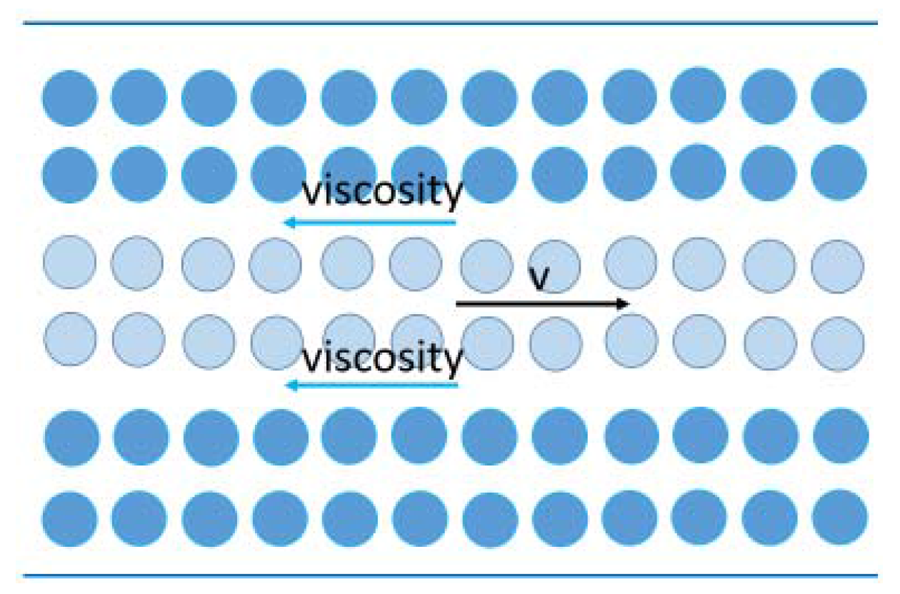
Viscosity, which is defined as the resistance of a fluid to flow, is essentially friction forces (Figure 1). For incompressible flow, the viscous stress tensor is , where is the viscosity and is the strain rate tensor. The shear rate is approximated by using Frobenius norm to model non-Newtonian fluids.
3.2. Carreau-Yasuda Model
Both Newtonian and non-Newtonian fluid flows are considered in this paper, and the variable viscosity under shear stress is achieved using a rheological model known as Carreau-Yasuda model [32]. The relationship between shear rate and viscosity is defined by:
where controls the shear rate and governs smoothness of transitions, and are given positive constants. When , the fluid is a Newtonian fluid with viscosity . When , the kinematic viscosity is equivalent to , which means under low shear rate, the viscosity of non-Newtonian fluid is governed by . When , the second term approaches zero and the viscosity approaches to as the shear rate increases, the simulated fluid is shear thinning non-Newtonian fluid. When , the viscosity increases with the amount of scaled by as the shear rate increases, and the simulated fluid is shear thickening non-Newtonian fluid.
3.3. Smoothed Particle Hydrodynamics
In the SPH approach, the basic idea is to discretize the fluid domain into a finite number of particles with physical attributes (Figure 2). A continuous field A(xi) can be obtained by summation over all the sampling points xj with mass mj and density pj in the support domain:
where is the kernel function with the particle radius, and iterating all the neighbors. The chosen kernel function is limited by several conditions, such as normalization, compact condition, and delta function property. In this paper, the popular quantic spline kernel is used for all simulations.
In the SPH interpolation scheme, the derivatives of field quantities only affect the smoothing kernel. The gradient of can be calculated as:
By substituting density into Equation (5), the density at location is:
Generally, there are two formulas to relate pressure and density, namely the Poisson equation and the gas state equation. Solving the Poisson equation guarantees the incompressibility of fluid, but it is time-consuming. In contrast, the explicit calculation is adopted in an ideal gas equation, but results in the stiffness value having to be very large so that the density fluctuations will not exceed 1%. However, according to the Courant-Friedrichs-Levy (CFL) condition, a large stiffness value will restrict the time step and make the simulation inefficient. In this paper, the equation of the gas state is used for efficiency and the problem of the stiffness value will be solved by pressure projection:
where is a gas constant that depends on the temperature, and is the rest density. The value turns out to be suitable for all experiments.
To compute the pressure acceleration, substitute into Equation (6):
In order to compute the shear stress at particle , the same SPH approximation as [33] is adopted for the deformation tensor with:
where . After updating shear stress at all particles, the viscous acceleration is approximated by:
4. Pressure Projection Algorithm
In the non-Newtonian fluid model proposed above, due to a rather high compressibility caused by the gas state equation, when a non-Newtonian fluid flows, the volume of the fluid might change [31]. In order to address this problem, a pressure projection algorithm is proposed to correct density by pressure.
Currently, there are many different pressure solvers that minimize the density error [28,29]. The algorithm proposed in this paper is similar with [28]. Firstly, only external force is considered to obtain the first intermediate velocity . Secondly, to enforce fluid incompressibility, a pressure projection algorithm is proposed in this section by using a new solver that sets a separate stiffness parameter for each fluid particle to satisfy local incompressibility, making the density of the entire fluid system remain unchanged and getting the second intermediate velocity . Next, an implicit method is proposed to solve the viscous stress tensor (see Section 5).
Finally, particle velocity and position are integrated using the Euler scheme, and the velocity can be rewritten as: with unknown pressure forces and viscosity forces and known external forces such as gravity and surface tension. Following the projection concept, intermediate (predicted) velocities are set to be :
The second intermediate velocity is:
The velocity in the next time step can be written as:
The pressure gradient is computed using the SPH formulation [29]:
The pressure force of particle caused by pressure acceleration is determined by:
is the pressure forces that act from particle on the neighboring particles . According to Newton’s third law, its value is equal to the total pressure of all neighboring particles affects , which satisfies . Then we can get:
The velocity changes by pressure forces is:
Similarly:
According to [28], the intermediate density caused by intermediate velocity is:
We now search for pressure forces to resolve the compression, i.e., the deviation from the rest density :
Solving for yields:
| Algorithm 1. Pressure Projection Algorithm |
| for all particles do update using Equation (7) update using Equation (21) end for for all particles do update using Equation (12) end for while () or do for all particles do update using Equation (20) update using Equation (21) end for end while for all particles do end for |
Algorithm 1 outlines the simulation using our novel method in detail. First, the particle neighborhoods using compact hashing [34] are determined. Then for each particle, the density and the factor are computed. Since this factor solely depends on the current positions, it is pre-computed before executing the solvers, which saves the solver from significant computational work. The third step in the simulation loop is to compute the strain tensor term of a non-Newtonian fluid, which is the main difference between a Newtonian fluid and a non-Newtonian fluid.
The forth and the fifth step of the algorithm are predictive-correction steps, whose purpose is to minimize the density error by the pressure solver, scilicet solving . In this step, the non-pressure forces are used to compute predicted velocities . The constant density solver uses this prediction and the pre-computed factors to determine the pressure forces for each neighborhood in order to correct the density error.
Finally, the resulting velocity changes are used to update the velocity of the particle without viscosity force .
5. Implicit Viscosity Solver
The viscous acceleration is commonly computed from the divergence of viscous stress tensor, which is mentioned in Section 3.2. In this paper, the proposed solver first computes an intermediate velocity without considering pressure and viscosity. Then, the second updated intermediate velocity is computed by using the proposed pressure correction method, which is described in Section 4. Finally, the proposed viscosity solver computes the final velocity and the position of particles. Algorithm 2 summarizes the proposed implicit non-Newtonian SPH fluid solver.
| Algorithm 2. Implicit non-Newtonian SPH fluid solver |
| for all particles do find neighborhoods compute time step size end for for all particles do compute the external force end for for all particles do update velocity end for for all particles do compute the external force end for for all particles do update velocity end for for all particles do compute the pressure and pressure force end for for all particles do update velocity // Pressure Projection end for for all particles do solving viscosity system end for for all particles do end for |
According to Algorithm 2, the viscosity solver starts with the strain rate tensor to compute the final velocity. Substituting Equation (15) into the strain rate tensor , and then getting the symmetric tensor for particle as a six-dimensional vector yields:
To solve the viscous acceleration , the gradient of viscous stress tensor should be computed:
According to the Equation (4), is the function of the strain rate tensor , while , , , and are given positive constants and will not influence the gradient computing. Thus, the gradient of viscous stress tensor can be written as:
Due to the formulation, the required derivatives of the strain rate tensor with respect to the velocity are determined by the following matrix:
In the SPH scheme, the derivatives of the strain rate tensor with respect to the velocity can be written as:
Now that all the variable quantities in Equation (14) can be solved, the final velocity and position of each particle are gained.
6. Implementation and Results
All timings are given for an Intel 3.50 GHz CPU with four cores. The simulation software is parallelized with Open MP. The simulation and surface reconstruction are actualized with C++ language and multi-threading technology. The density fluctuation was set to 0.01.
Figure 3 shows the Newtonian fluid and non-Newtonian fluid according to our method. As described in Section 3.2, when , the non-Newtonian fluid model is simplified to a Newtonian fluid with constant kinematic viscosity (Figure 3a). When the fluid touches the container at the bottom of the scene (the container is set to be transparent for observers’ convenience), the fluid particles that touch the container splash upward. In contrast, the non-Newtonian fluid particles (shown in Figure 3b) cannot splash when they collide with container due to their viscosity. The setting and statistics are illustrated in Table 1.
Figure 4 shows the free fall of a water column in particle state with 13,671 particles. In the same initial scene, both Newtonian fluid (Figure 4a) and non-Newtonian fluid (Figure 4b) could be achieved by governing the coefficients. We compared the non-Newtonian fluid simulation of our method with the method of Andrade et al. [25]. Andrade et al. used explicit integration without pressure projection. During the experiment, when the scene was small or the fluid particles moved gently, running the algorithm with pressure correction was found to be time and memory-consuming. However, when the scene is large or the fluid particles collide intensely, the method of Andrade et al. will be unstable with the larger time step. As shown in Figure 4c, when the time step was set to 3.0 × 10⁻⁴ s, fluid particles scattered in all directions with the method of Andrade et al. [25], while our algorithm still ran with the pressure projection (Figure 4d).
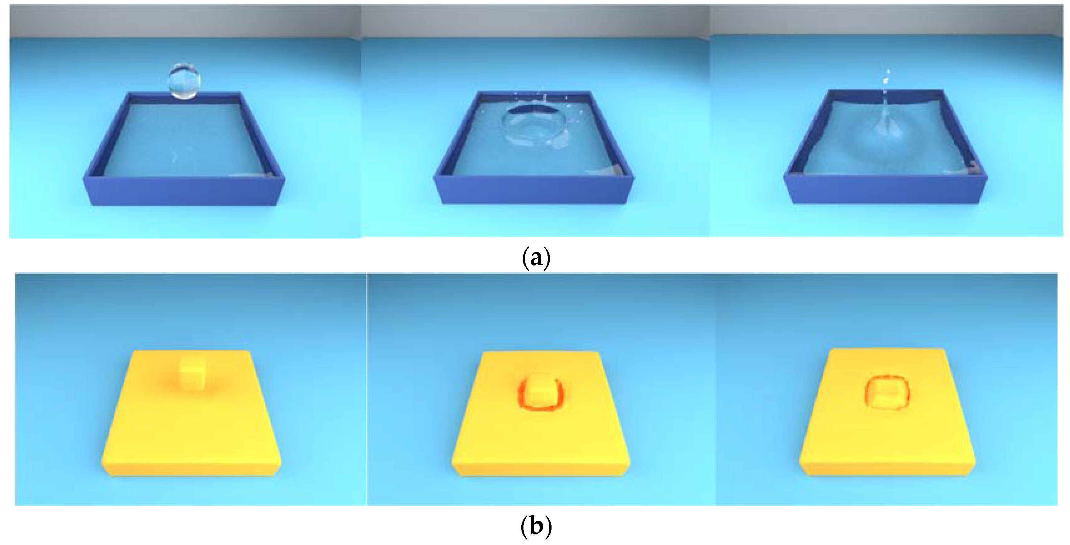
Figure 5 shows a water ball falling in a pool. The first line is Newtonian fluid (Figure 5a) and the second line is the non-Newtonian fluid (Figure 5b). As can be seen from the pictures, the wave of Newtonian fluid lashed against the water, sending up pearly spray. For the non-Newtonian fluid, there is no wave and the water sank into the pool directly. The setting and statistics are illustrated in Table 2.
At our test scene (Figure 4), we compared the simulation times and stability of our method with the method of Andrade et al. [25]. The physical parameters and performance measurements are summarized in Table 3. For the explicit method without pressure projection (Andrade et al. [25]), the time step is set according to the CFL condition [35] and the viscosity of fluid [25]. In the case of η = 0.01, the time step of our method could be running well with Δt = 3.0 × 10⁻⁴ s, while the method of Andrade et al. [25] could not. As a result, for a two-second animation, our method needs 32 frames and 44.5 min for computing, while the method of Andrade et al. [25] needs 67 frames and 59.5 min for computing. The simulation parameters and performance of Figure 4 are also listed in Table 3.
7. Conclusions
In this paper, we proposed a novel symmetry particle-based method for non-Newtonian fluid, where the variable viscosity is decided by the Carreau-Yasuda Model. Our method includes a pressure correction step to reduce the density errors and ensure the incompressibility of fluid. An implicit method is used for the non-Newtonian fluid simulation to improve efficiency and stability. With our method, the fluid simulation runs well in large time steps compared with previous work.
One limitation of our method is that it does not consider temperature in our non-Newtonian fluid model. By taking this into fluid model, one could begin to simulate phenomena of solid-liquid conversion, like wax melt in high temperature. Additionally, work remains to be done on the topic of multi-phase coupling between different non-Newtonian fluids. This might be a potential direction for future work.
Acknowledgments
This work was supported by National Natural Science Foundation of China (No. 61572075) and The National Key Research and Development Program of China (Grant Nos. 2016YFB0700502, 2016YFB1001404).
Author Contributions
Yalan Zhang conceived the framework and wrote the paper; Xing Liu performed the experiments; Xiaokun Wang checked the results; all the work was done under the guidance of Xiaojuan Ban.
Conflicts of Interest
The authors declare no conflict of interest.
References
- Ellero, M.; Tanner, R.I. SPH simulations of transient viscoelastic flows at low Reynolds number. J. Non-Newton. Fluid Mech. 2005, 132, 61–72. [Google Scholar] [CrossRef]
- Müller, M.; Charypar, D.; Gross, M. Particle-based fluid simulation for interactive applications. In Proceedings of the 2003 ACM SIGGRAPH/Eurographics Symposium on Computer Animation, San Diego, CA, USA, 26–27 July 2003; Eurographics Association Press: Aire-la-Ville, Switzerland, 2003; pp. 154–159. [Google Scholar]
- Shadloo, M.S.; Oger, G.; Le Touzé, D. Smoothed particle hydrodynamics method for fluid flows, towards industrial applications: Motivations, current state, and challenges. Comput. Fluids 2016, 136, 11–34. [Google Scholar] [CrossRef]
- Sadek, S.H.; Yildiz, M. Modeling Die Swell of Second-Order Fluids Using Smoothed Particle Hydrodynamics. J. Fluids Eng. 2013, 135, 051103. [Google Scholar] [CrossRef]
- Zainali, A.; Tofighi, N.; Shadloo, M.S.; Yildiz, M. Numerical investigation of Newtonian and non-Newtonian multiphase flows using ISPH method. Comput. Methods Appl. Mech. Eng. 2013, 254, 99–113. [Google Scholar] [CrossRef]
- Price, D.J. Modelling discontinuities and Kelvin–Helmholtz instabilities in SPH. J. Comput. Phys. 2008, 227, 10040–10057. [Google Scholar] [CrossRef]
- Hayhurst, C.J.; Clegg, R.A. Cylindrically symmetric SPH simulations of hypervelocity impacts on thin plates. Int. J. Impact Eng. 1997, 20, 337–348. [Google Scholar] [CrossRef]
- Omang, M.; Børve, S.; Trulsen, J. Alternative kernel functions for Smoothed Particle Hydrodynamics in cylindrical symmetry. Shock Waves 2005, 14, 293–298. [Google Scholar] [CrossRef]
- Ren, J.; Ouyang, J.; Jiang, T.; Li, Q. A corrected symmetric SPH method to simulate viscoelastic free surface flows based on the PTT model. Int. J. Numer. Methods Fluids 2012, 70, 1494–1517. [Google Scholar] [CrossRef]
- Monaghan, J.J. Simulating free surface flows with SPH. J. Comput. Phys. 1994, 110, 399–406. [Google Scholar] [CrossRef]
- Shao, S.; Lo, E.Y.M. Incompressible SPH method for simulating Newtonian and non-Newtonian flows with a free surface. Adv. Water Resour. 2003, 26, 787–800. [Google Scholar] [CrossRef]
- Bridson, R.; Fedkiw, R.; Müller-Fischer, M. Fluid simulation: SIGGRAPH 2006 course notes Fedkiw and Muller-Fischer presenation videos are available from the citation page. In Proceedings of the SIGGRAPH '06 Special Interest Group on Computer Graphics and Interactive Techniques Conference, Boston, MA, USA, 30 July–3 August 2006.
- Goktekin, T.G.; Bargteil, A.W.; O’Brien, J.F. A Method for Animating Viscoelastic Fluids. ACM Trans. Graph. 2004, 23, 461–466. [Google Scholar] [CrossRef]
- Losasso, F.; Shinar, T.; Selle, A.; Fedkiw, R. Multiple interacting liquids. ACM Trans. Graph. 2006, 25, 812–819. [Google Scholar] [CrossRef]
- Batty, C.; Bridson, R. Accurate Viscous Free Surfaces for Buckling, Coiling, and Rotating Liquids. In Proceedings of the 2008 Eurographics/ACM SIGGRAPH Symposium on Computer Animation, SCA 2008, Dublin, Ireland, 7–9 July 2008; pp. 219–228.
- Bergou, M.; Audoly, B.; Vouga, E.; Wardetzky, M.; Grinspun, E. Discrete viscous threads. ACM Trans. Graph. 2010, 29, 157–166. [Google Scholar] [CrossRef]
- Batty, C.; Uribe, A.; Audoly, B.; Grinspun, E. Discrete Viscous Sheets. ACM Trans. Graph. 2012, 31, 13–15. [Google Scholar] [CrossRef]
- Xu, X.; Ouyang, J.; Yang, B.; Liu, Z. SPH simulations of three-dimensional non-Newtonian free surface flows. Comput. Methods Appl. Mech. Eng. 2013, 256, 101–116. [Google Scholar] [CrossRef]
- Pan, W.; Tartakovsky, A.M.; Monaghan, J.J. Smoothed particle hydrodynamics non-Newtonian model for ice-sheet and ice-shelf dynamics. J. Comput. Phys. 2013, 242, 828–842. [Google Scholar] [CrossRef]
- Müller, M.; Keiser, R.; Nealen, A.; Pauly, M.; Gross, M.; Alexa, M. Point based animation of elastic, plastic and melting objects. In Proceedings of the ACM Siggraph/eurographics Symposium on Computer Animation, Grenoble, France, 27–29 August 2004; Eurographics Association: Aire-la-Ville, Switzerland, 2004; pp. 141–151. [Google Scholar]
- Afonso, P.; Fabiano, P.; Thomas, L.; Geovan, T. Particle-based viscoplastic fluid/solid simulation. Comput.-Aided Des. 2009, 41, 306–314. [Google Scholar]
- Paiva, A.; Petronetto, F.; Lewiner, T.; Tavares, G. Particle-based non-Newtonian fluid animation for melting objects. In Proceedings of the 2006 19th Brazilian Symposium on Computer Graphics and Image Processing, Manaus, Brazil, 8–11 October 2006; pp. 78–85.
- Rafiee, A.; Manzari, M.T.; Hosseini, M. An incompressible SPH method for simulation of unsteady viscoelastic free-surface flows. Int. J. Non-Linear Mech. 2007, 42, 1210–1223. [Google Scholar] [CrossRef]
- Fan, X.J.; Tanner, R.I.; Zheng, R. Smoothed particle hydrodynamics simulation of non-Newtonian moulding flow. J. Non-Newton. Fluid Mech. 2010, 165, 219–226. [Google Scholar] [CrossRef]
- De Andrade, L.F.S.; Sandim, M.; Petronetto, F.; Pagliosa, P.; Paiva, A. SPH Fluids for Viscous Jet Buckling. In Proceedings of the Graphics, Patterns and Images, Rio de Janeiro, Brazil, 26–30 August 2014; pp. 65–72.
- Zhang, Y.; Ban, X.; Wang, X.; Liu, X. A Density-Correction Method for Particle-Based Non-Newtonian Fluid. In Cooperative Design, Visualization, and Engineering; Springer: Heidelberg, Germany, 2016. [Google Scholar]
- Zhu, B.; Lee, M.; Quigley, E.; Fedkiw, R. Codimensional non-Newtonian fluids. ACM Trans. Graph. 2015, 34, 1–9. [Google Scholar] [CrossRef]
- Solenthaler, B.; Pajarola, R. Predictive-corrective incompressible SPH. ACM Trans. Graph. 2009, 28, 341–352. [Google Scholar] [CrossRef] [Green Version]
- Ihmsen, M.; Cornelis, J.; Solenthaler, B.; Horvath, C.; Teschner, M. Implicit Incompressible SPH. IEEE Trans. Vis. Comput. Graph. 2014, 20, 426–435. [Google Scholar] [CrossRef] [PubMed]
- Bender, J.; Koschier, D. Divergence-free smoothed particle hydrodynamics. In Proceedings of the 14th ACM SIGGRAPH/Eurographics Symposium on Computer Animation, Los Angeles, CA, USA, 07–09 August 2015; Eurographics Association Press: Aire-la-Ville, Switzerland, 2015; pp. 147–155. [Google Scholar]
- Becker, M.; Teschner, M. Weakly compressible SPH for free surface flows. In Proceedings of the ACM Siggraph/eurographics Symposium on Computer Animation, SCA 2007, San Diego, CA, USA, 2–4 August 2007; pp. 209–217.
- Macosko, C.W.; Larson, R.G. Rheology: Principles, Measurements, and Applications; Wiley: New York, NY, USA, 1994. [Google Scholar]
- Morris, J.P.; Fox, P.J.; Zhu, Y. Modeling low Reynolds number incompressible flows using SPH. J. Comput. Phys. 1997, 136, 214–226. [Google Scholar] [CrossRef]
- Ihmsen, M.; Akinci, N.; Becker, M.; Matthias, T. A Parallel SPH Implementation on Multi-Core CPUs. Comput. Graph. Forum 2011, 30, 99–112. [Google Scholar] [CrossRef]
- Monaghan, J.J. Smoothed particle hydrodynamics. Annu. Rev. Astron. Astrophys. 1992, 30, 543–574. [Google Scholar] [CrossRef]
Figure 1.
Viscous forces model. V: velocity.

Figure 2.
Illustration for smoothed particle hydrodynamics (SPHs) method. It is a symmetry particle method and the physical attributions of each particle is weighted in summation by its neighbors.
Figure 2.
Illustration for smoothed particle hydrodynamics (SPHs) method. It is a symmetry particle method and the physical attributions of each particle is weighted in summation by its neighbors.
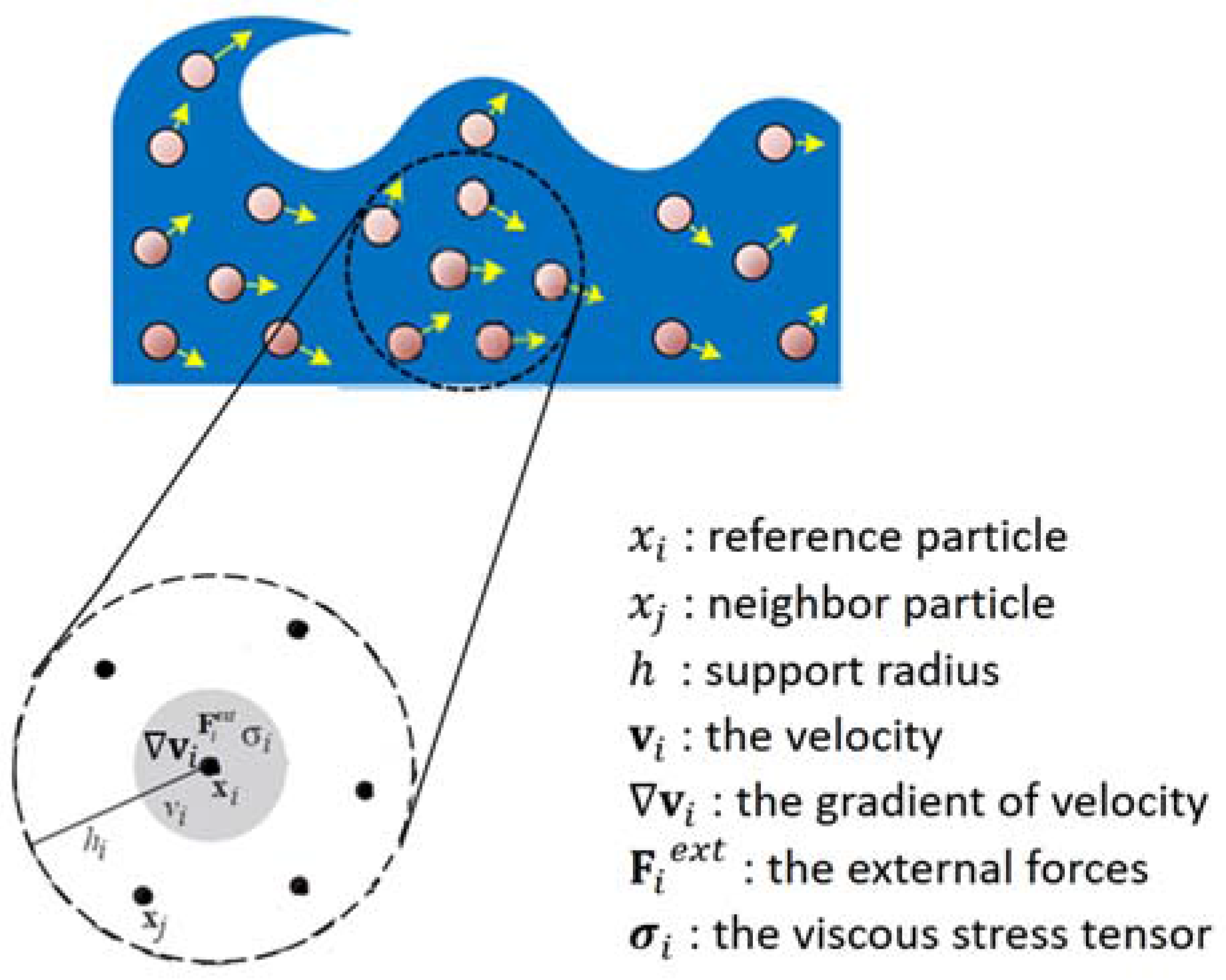
Figure 3.
A falling water column with our method. (a) is Newtonian fluid; (b) is the non-Newtonian fluid.
Figure 3.
A falling water column with our method. (a) is Newtonian fluid; (b) is the non-Newtonian fluid.
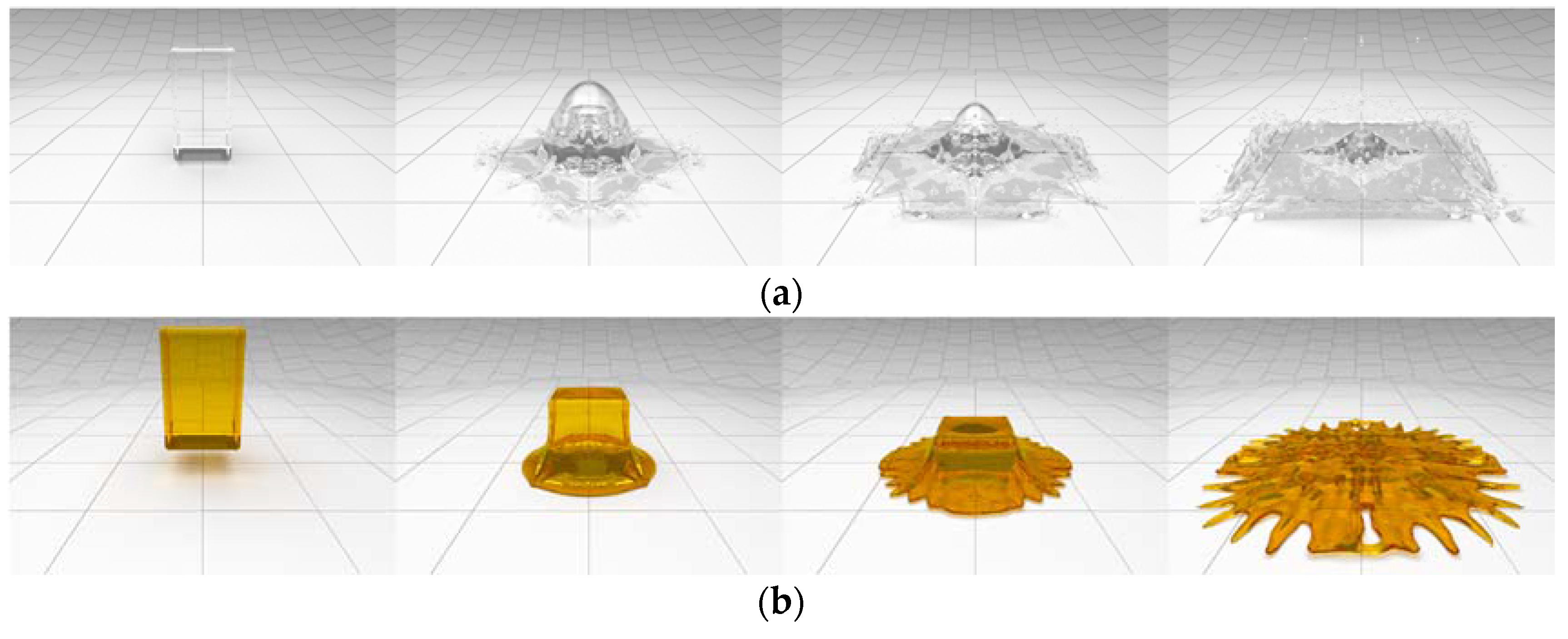
Figure 4.
The free fall of a water column. (a) is Newtonian fluid (our method); (b) is the non-Newtonian fluid (Andrade et al. [25]) with ; (c) is the non-Newtonian fluid (Andrade et al. [25]) with ; (d) is the non-Newtonian fluid (our method) with .
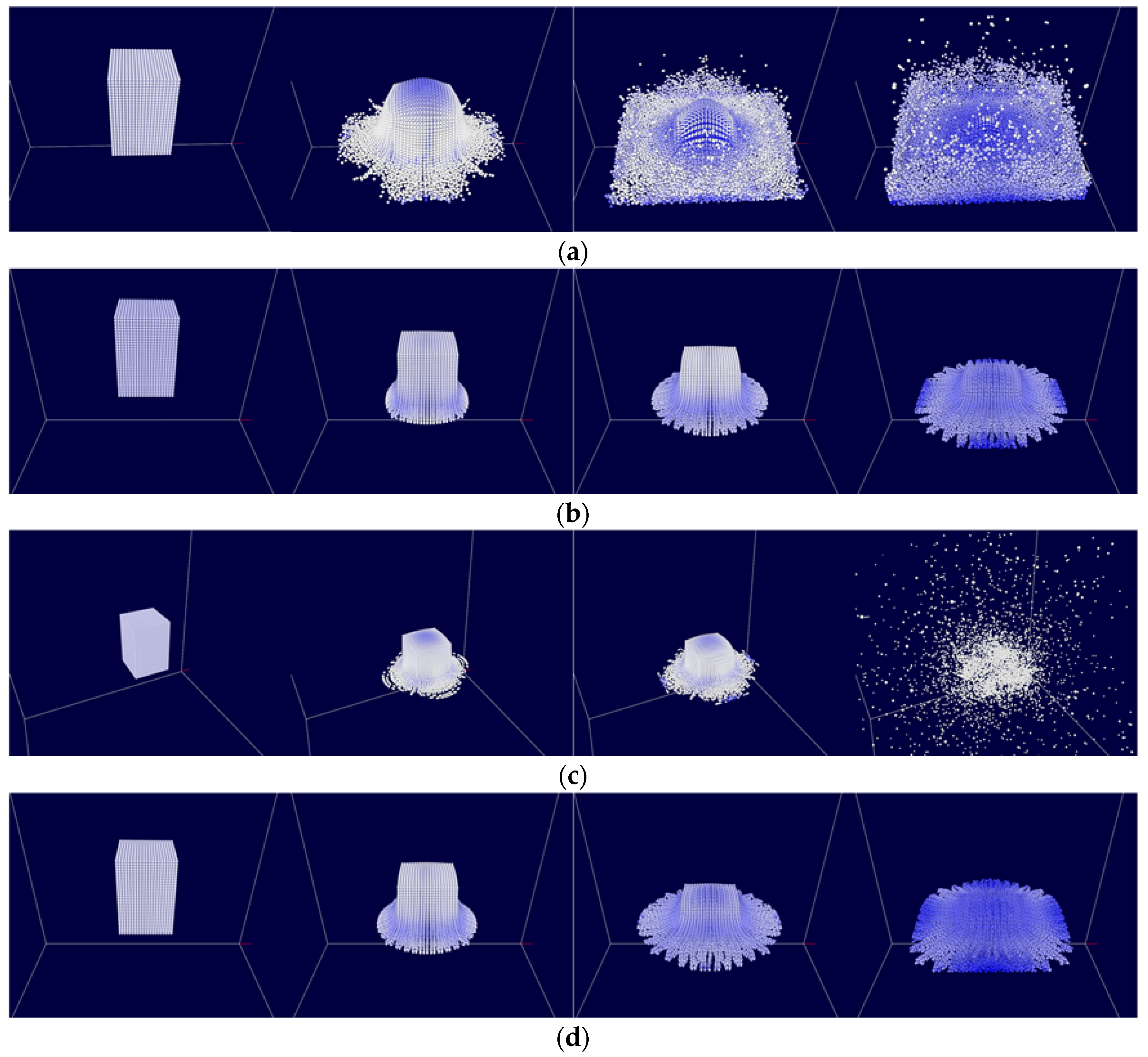
Figure 5.
A water block falling in a pool. (a) is Newtonian fluid; (b) is the non-Newtonian fluid.

Table 1.
The simulation parameters for Figure 3. (Both Newtonian and non-Newtonian fluid).
| Simulation domain size | 6 m × 6 m × 6 m |
| Fluid particles | 13,671 |
| Smoothing kernel function | cubic splines |
| Smoothing radius | 0.1 m |
| Fluid particle width | 0.05 m |
| Rendering time(per frame) | 1.14 min |
Table 2.
The simulation parameters for Figure 5. (Both Newtonian and non-Newtonian fluid).
| Simulation domain size | 8 m × 8 m × 8 m |
| Fluid particles | 32,751 |
| Smoothing kernel function | cubic splines |
| Smoothing radius | 0.2 m |
| Fluid particle width | 0.1 m |
| Rendering time(per frame) | 3.85 min |
Table 3.
The simulation parameters and performance. , , , and : fluid physical parameters, : time step, : simulation time per frame.
| Figure | |||||||
|---|---|---|---|---|---|---|---|
| Figure 4a | - | 0.2 | - | - | 1 | 3.0 × 10⁻⁴ | 40.8 |
| Figure 4b | 2 | 0.2 | 1 | 0.5 | −0.5 | 2.5 × 10⁻⁶ | 53.3 |
| Figure 4c | 2 | 0.2 | 1 | 0.5 | −0.5 | 3.0 × 10⁻⁴ | - |
| Figure 4d | 2 | 0.2 | 1 | 0.5 | −0.5 | 3.0 × 10⁻⁴ | 83.4 |
| Figure 5a | - | 0.2 | - | - | 1 | 6.0 × 10⁻⁴ | 178 |
| Figure 5b | 0.2 | 2 | 1 | 0.5 | −0.5 | 6.0 × 10⁻⁴ | 216 |
© 2017 by the authors. Licensee MDPI, Basel, Switzerland. This article is an open access article distributed under the terms and conditions of the Creative Commons Attribution (CC BY) license ( http://creativecommons.org/licenses/by/4.0/).
Share and Cite
MDPI and ACS Style
Zhang, Y.; Ban, X.; Wang, X.; Liu, X. A Symmetry Particle Method towards Implicit Non‐Newtonian Fluids. Symmetry 2017, 9, 26. https://doi.org/10.3390/sym9020026
AMA Style
Zhang Y, Ban X, Wang X, Liu X. A Symmetry Particle Method towards Implicit Non‐Newtonian Fluids. Symmetry. 2017; 9(2):26. https://doi.org/10.3390/sym9020026
Chicago/Turabian StyleZhang, Yalan, Xiaojuan Ban, Xiaokun Wang, and Xing Liu. 2017. "A Symmetry Particle Method towards Implicit Non‐Newtonian Fluids" Symmetry 9, no. 2: 26. https://doi.org/10.3390/sym9020026
Note that from the first issue of 2016, this journal uses article numbers instead of page numbers. See further details here.