
Generalized Degree-Based Graph Entropies

School of Statistics and Mathematics, Zhongnan University of Economics and Law, No. 182 Nanhu Avenue, Wuhan 430073, China
Symmetry 2017, 9(3), 29; https://doi.org/10.3390/sym9030029
Submission received: 23 November 2016
/
Revised: 17 February 2017
/
Accepted: 20 February 2017
/
Published: 28 February 2017
(This article belongs to the Special Issue Symmetry in Complex Networks II)
Abstract
:Inspired by the generalized entropies for graphs, a class of generalized degree-based graph entropies is proposed using the known information-theoretic measures to characterize the structure of complex networks. The new entropies depend on assigning a probability distribution about the degrees to a network. In this paper, some extremal properties of the generalized degree-based graph entropies by using the degree powers are proved. Moreover, the relationships among the entropies are studied. Finally, numerical results are presented to illustrate the features of the new entropies.
1. Introduction
Nowadays, the research of complex networks has attracted many researchers. One interesting and important problem is to study the network structure by using different graph and network measures. Meanwhile, these graph and network measures have been widely applied in many different fields, such as chemistry, biology, ecology, sociology and computer science [1,2,3,4,5,6,7]. From the viewpoint of information theory, the entropy of graphs was initiated to be applied by Mowshowitz [8] and Trucco [9]. Afterwards, Dehmer introduced graph entropies based on information functionals which capture structural information and studied their properties [10,11,12]. The graph entropies have been used as the complexity measures of networks and measures for symmetry analysis. Recently, so-called generalized graph entropies have been investigated by Dehmer and Mowshowitz [13] for better analysis and applications such as machine learning. The generalized graph entropies can characterize the topology of complex networks more effectively [14].
The degree powers are extremely considerable invariants and studied extensively in graph theory and network science, so they are commonly used as the information functionals to explore the networks [15,16]. To study more properties of graph entropies based on the degree powers, Lu et al. obtained some upper and lower bounds which have different performances to bound the graph entropies in different kinds of graphs and showed their applications in structural complexity analysis [17,18]. Inspired by Dehmer and Mowshowitz [13], we focus on the relationships between degree powers and the parametric complexity measures and then we construct generalized degree-based graph entropies by using the concept of the mentioned generalized graph entropies. The structure of this paper is as follows: In Section 2, some definitions and notations of graph theory and the graph entropies we are going to study are reviewed. In Section 3, we describe the definition of generalized degree-based graph entropies which are motivated by Dehmer and Mowshowitz [13]. In Section 4, we present some extremal properties of such entropies related to the degree powers. Moreover, we give some inequalities among the generalized degree-based graph entropies. In Section 5, numerical results of an exemplary network are shown to demonstrate the new entropies. Finally, a short summary and conclusion are drawn in the last section.
2. Preliminaries to Degree-Based Graph Entropy
A graph or network G is an ordered pair comprising a set V of vertices together with a set E of edges. In network science, vertices are called nodes sometimes. The order of a graph means the number of vertices. The size of a graph means the number of edges. A graph of order n and size m is recorded as an -graph. The degree of a vertex v denoted by or in short means the number of edges that connect to it, where an edge that connects a vertex to itself (a loop) is counted twice. The maximum and minimum degree in a graph are often denoted by and . If every vertex has the same degree (), then G is called a regular graph, or is called a d-regular graph with vertices of degree d. An unordered pair of vertices is called connected if a path leads from u to v. A connected graph is a graph in which every unordered pair of vertices is connected. Otherwise, it is called a disconnected graph. Obviously, in a connected graph, . A tree is a connected graph in which any two vertices are connected by exactly only one path. So tree is a connected -graph. is denoted a path graph characterized as a tree in which the degree of all but two vertices is 2 and the degree of the two remaining vertices is 1. is denoted a star graph characterized as a tree in which the degree of all but one vertex is 1. More details can be seen in [17,18].
Next, we describe the concept of (Shannon’s) entropy [19,20]. The notation “log” means the logarithm is based 2, and the notation “ln” means the logarithm is based .
Definition 1.
Let be a probability distribution, namely, and . The (Shannon’s) entropy of the probability distribution is defined by
In the above definition, we use for continuity of corresponding function.
Definition 2.
Let be a graph of order n. For , we define
where f is a meaningful information functional. According to the information functional f, the vertices are mapped to the non-negative real numbers.
Because , the quantities can be seen as probability values. Then the graph entropy of G has been defined as follows [10,12,17,18].
Definition 3.
Let be a graph of order n and f be a meaningful information functional. The (Shannon’s) graph entropy of G is defined by
Definition 4.
Let be a graph of order n. For , if , then
Therefore, the degree-based graph entropy of G is defined as
3. Generalized Degree-Based Graph Entropy
Many generalizations of entropy measure have been proposed based on the definition of Shannon’s entropy [21,22]. For example, Rényi entropy [23], Daròczy’s entropy [24] and quadratic entropy [25] are representative generalized entropies. In [13], Dehmer and Mowshowitz introduce a new class of generalized graph entropies that derive from the generalizations of entropy measure mentioned above and present two examples.
Definition 5.
Let be a graph of order n. Then
Definition 6.
Let be a graph of order n and A its adjacency matrix. Denote by the eigenvalues of G. If , then the generalized graph entropies are as follows:
Definition 7.
Let be a graph of order n. Denote the collection of orbits by and their respective probabilities by , where k is the number of orbits. Then another class of generalized graph entropies are derived as
Because it is difficult to obtain the eigenvalues or the collection of orbits of graph G for a large-scale graph, and they may not meet the requirements visually, we focus on the complexity of the graphs or networks determined by the vertices themselves and the relationship between them in this paper. For a given graph G, the vertex degree is a significant graph invariant, which is related to structural properties of the graph. Most other properties of the complex network are based on the degree distribution, such as the clustering coefficient, the community structure and so on. The vertex degree in a graph or network is also intuitional and noticeable. The vertices with varying values of degree chosen as the main construction of the graph or network may decide the complexity of the graph or network. Hence, we study the generalized graph entropies based on the vertex degree and degree powers.
According to the above definitions of generalized graph entropies, let for , then we obtain the generalized degree-based graph entropies as follows:
Definition 8.
4. Properties of the Generalized Degree-Based Graph Entropies
In this section, we will show the relationships among the stated generalized degree-based graph entropies and the degree-based graph entropy. First we will present five simple propositions which can be inferred from the Rényi entropy and [13].
Proposition 1.
Proof.
Remark 1.
Proposition 1 can be seen as a special case of (12) and (16) in [13] when the value of the information functional is the degree of every vertex.
Proposition 2.
Proof.
Using l’Hôspital’s rule, we can obtain the Equation (7). ☐
Proposition 3.
For , is monotonically decreasing with respect to α.
Proof.
The derivative of the function is
where , . Then and are also probability distributions. From the nonnegativity of Kullback-Leibler divergence, we obtain . The inequality implies that is monotonically decreasing with respect to α. ☐
Proposition 4.
For ,
and for ,
Proof.
Using Proposition 2 and Proposition 3, we can obtain the equalities above easily. ☐
Remark 2.
Proposition 2, Proposition 3 and Proposition 4 can be seen as the special cases of the Rényi entropy’s properties.
Proposition 5.
Proof.
Using the standard inequality when , we have . Therefore,
Then the inequality (10) follows. ☐
Next we define the sum of the α-th degree powers as , where α is an arbitrary real number.
Theorem 1.
Let be an -graph. Then for , we have
From the above theorem, we know that the generalized degree-based graph entropies are closely related to the sum of the degree powers . Obviously when , presents the sum of degrees. The sum of the degree powers as an invariant is called zeroth order general Randić index [26,27,28,29]. For , is also called first Zagreb index [30,31,32,33]. In [34], Chen et al. have reviewed for different values of α and discussed the relationships with some indices such as Zagreb index, graph energies, HOMO-LUMO index, Estrada index [35,36,37,38,39,40,41,42,43].
Corollary 1.
Let be an -graph. Then we have
Proof.
Using Cauchy-Buniakowsky-Schwarz inequality, we obtain
In [44] de Caen obtains the following inequality
We can also find some conditions for the equalities: If G is a regular graph, then the equality holds; If G is a tree of order n, then the equality holds. ☐
Corollary 2.
Let T be a tree of order n. Then we have
where and denote the star graph and path graph of order n, respectively.
Proof.
In [45], Li and Zhao present that among all trees of order n, for or , the path graph and the star graph attain the minimum and maximum value of respectively; while for , the star graph and the path graph attain the minimum and maximum value of respectively. Then using the Equation (13), the result of the corollary is obtained. ☐
Theorem 2.
When , we have ; and when , we have . Especially, when , we have .
Proof.
First we define a new function on α on the set of real numbers as follows
Because straightforward derivative shows
we can claim that is a strictly decreasing function on α.
For , we have
Using the standard inequality when , we find when .
Therefore, for , we have
For , we have
Especially, when , and . So holds in this case. ☐
Corollary 3.
When , we have .
Proof.
First we define a new function on α on the set of real numbers as follows
Because the second order derivative shows
we can claim that is a convex function on α. Since , we find for , or equivalently for . Using Theorem 2, the inequality holds. ☐
Theorem 3.
When and , we have ; when , we have ; and when , we have .
Proof.
First we have
and is a strictly decreasing function on α.
Therefore, for , and are obtained. Then we have
This implies .
For , and are obtained. Then we have
This implies .
For , using (6) we have .
For , and are obtained. Then we have
This implies . Thus we complete the proof. ☐
Corollary 4.
When , we have .
Proof.
For , we have the result by using Theorem 3. ☐
Theorem 4.
When , we have ; when , we have ; and when , we have .
For , and are obtained. Then we have
Using the standard inequality when , we find . So
This implies .
For , using Theorem 2 and Theorem 3 we have and . This implies . Thus we complete the proof. ☐
5. Numerical Results
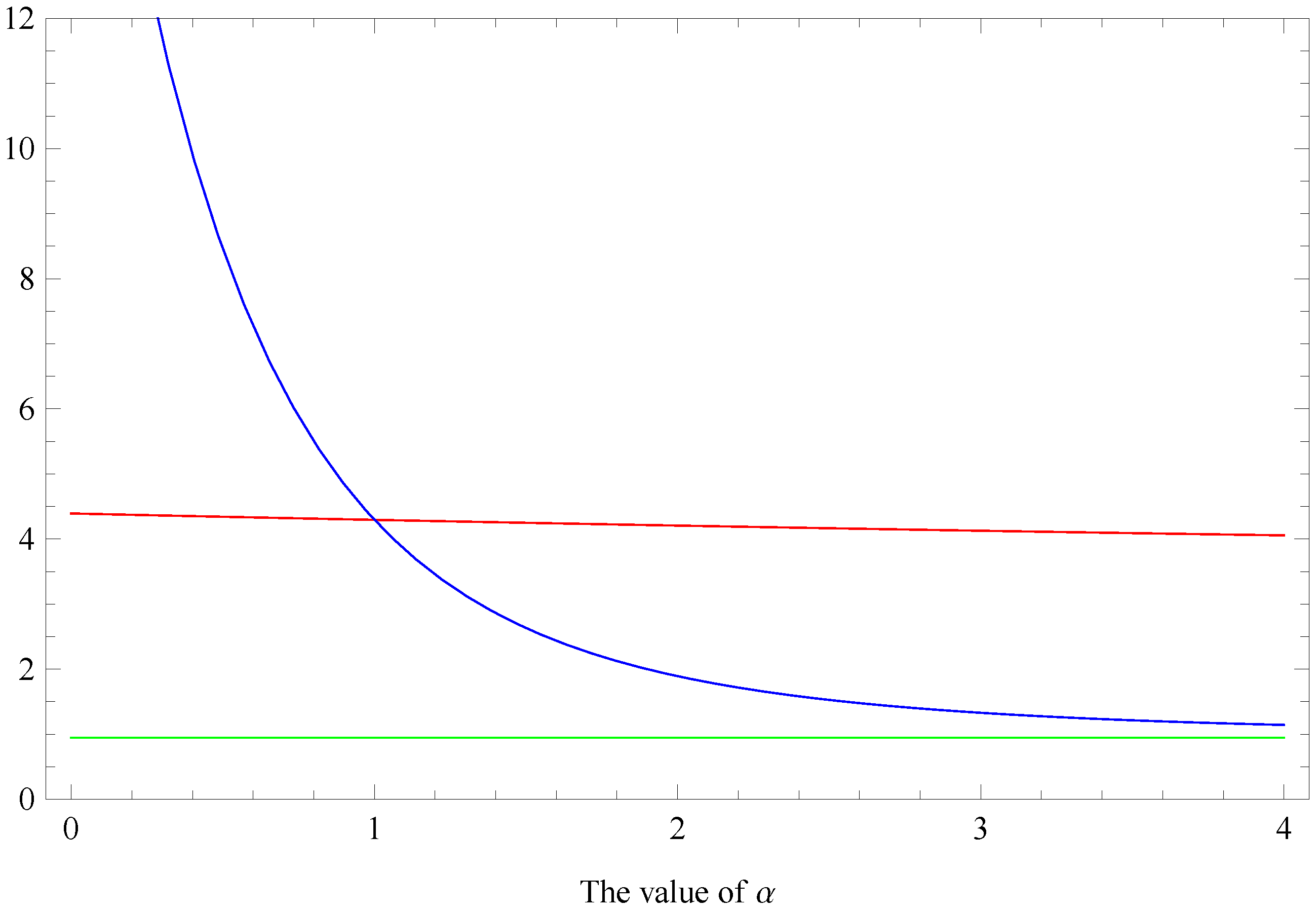
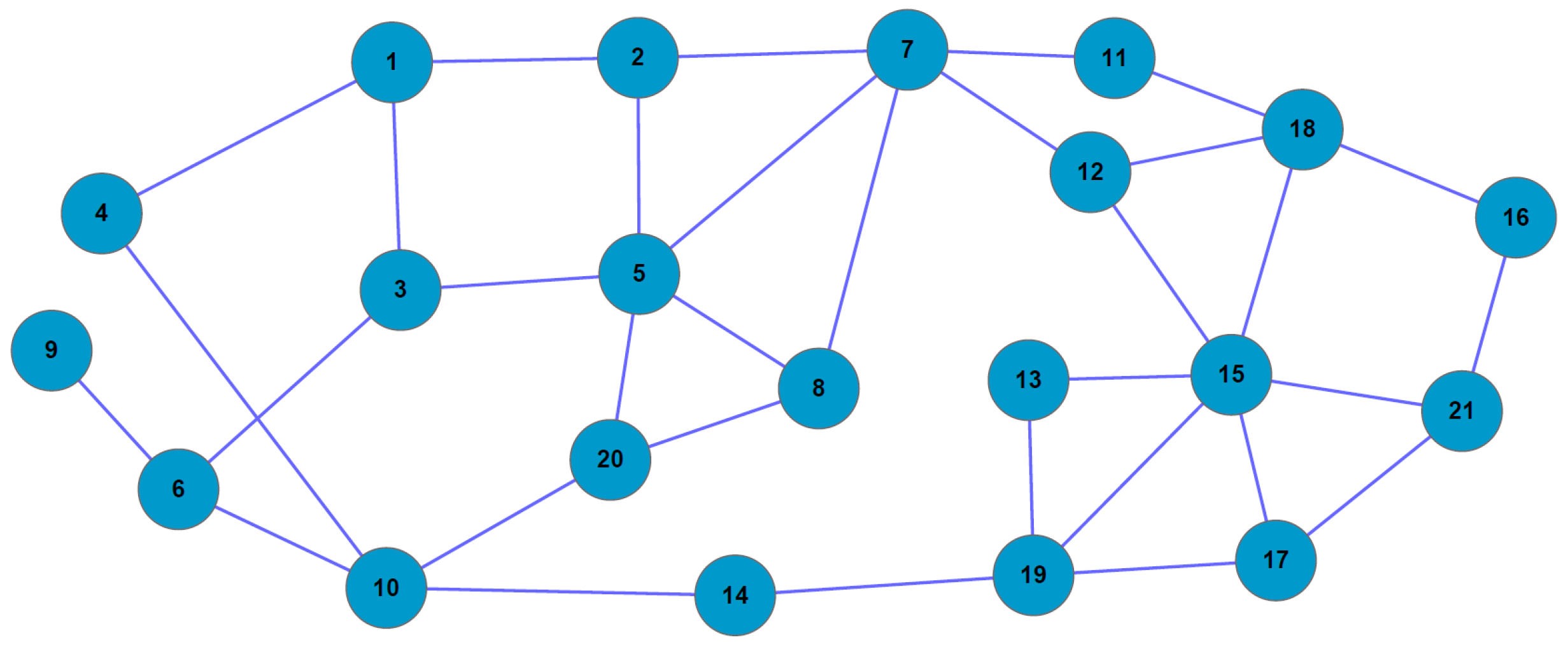
In order to illuminate the principle of generalized degree-based graph entropies, we show a network in Figure 1 as an example.
The degree of each node of the example network is shown in Table 1.
We can easily calculate . The details of and with different α are shown in Table 2.
In Table 2 that the value of α is equal to means . Then and are degenerated to the degree-based graph entropy .
It is clear that following the increase of the value of α, the values of the generalized degree-based graph entropies and of the complex network are decrease. Based on the concept of the entropy, the bigger the value of the entropy is, the more complex of the network is. From the definitions of and , the value of the entropic index α can be used to change the construction of the entropies. In other words, the value of α represents the relationship among the nodes in the complex network. Combined with the complex network, the influence of each node’s degree on the entropies is changed by the value of α. The relationship between the value of α and the entropies of the complex network is shown as follows:
- (1)
- When , the nodes with small value of degree play an important part in the construction of and , or they are chosen as the main construction of the complex networks. Especially when the value of , each node has the same influence on the whole network from the entropic point of view.
- (2)
- When , the influence of each node on the network is based on the value of degree for each node. The generalized degree-based graph entropies and are degenerated to the degree-based graph entropy . So the structure property determined by the node’s degree decides the complexity of the complex network.
- (3)
- When , the nodes with big value of degree play an important part in the construction of and , or they are chosen as the main construction of the complex networks. The values of the entropies tend to stabilization. The complex network is tended to orderly.
To sum up, according to the definition of the generalized degree-based graph entropies of the complex network, the value of the entropic index α is used to describe the different relationship among the nodes. When the value of α is smaller than 1, the nodes with small value of degree are more important than the nodes with big value of degree. The edges among those nodes with small value of degree become the main part of the complex network. As these nodes with small value of degree are the majority in the complex network, the whole network has greater complexity. When the value of α is equal to 0, the nodes in the network are equal to each other in terms of influence. When the value of α tends to 1, and are degenerated to , the level of complexity for the complex network is decided by the structure property. In other words, the complexity of the complex network is decided by the degree sequence and degree distribution. When the value of α is trended to ∞, the construction of the complex network is decided by the node which has a biggest value of degree, the values of and decrease to stable values, and the complex network is more orderly. The complexity of the complex network is not only decided by the structure of the complex network, but also influenced by the kind of the relationship between each node.
From Figure 2, we can see the plotted values of the generalized degree-based graph entropies , and relative to α (, with a pole at ). The numerical results can be interpreted as follows: First we observe that the value of is less than that of for , while the value of is larger than that of for . Next, for , and , we can have the values of and is always larger than that of . Actually, using l’Hôspital’s rule we have that the value of tends to 3.459 and the value of tends to 1 when α tends to . At last, all the curves verify the inequalities in the Section 4.
In addition, generalized graph entropy measures with parameters have been presented to be useful in studying the complexity associated with machine learning. For example, Dehmer et al. have described that the generalized graph entropies can be applied to the graph classification and clustering cases in machine learning. The applications involve optimizing particular parameters associated with graphs or networks in given sets [4,46]. So by applying supervised machine learning methods, the generalized degree-based entropies can be used for classifying the chemical structures, developing methods for characterizing predictive models according to optimal values of relevant parameters in bioinformatics, systems biology, and drug design.
6. Summary and Conclusions
In this paper , we studied the generalized degree-based graph entropies, which are inspired by Dehmer and Mowshowitz in [13] and derived from the Rényi entropy [23], Daròczy’s entropy [24] and quadratic entropy [25]. We studied the relationships between the sum of the degree powers and the new entropies. Then we examined the extremal values of the above stated entropies in terms of the sum of the degree powers. We also proved some inequalities between these generalized degree-based graph entropies. Finally, we obtained numerical values for an exemplary complex network for each of the entropies, and concluded that their parameters can influence which kind of nodes contribute to the main part of the network in terms of graph entropy theory. The generalized degree-based graph entropies expand the description methods of the structural complexity of the complex networks. They would play bigger roles in describing structural symmetry and asymmetry in real networks in the future.
Acknowledgments
The author would like to thank the editor and referees for their helpful suggestions and comments on the manuscript.
Conflicts of Interest
The author declares no conflict of interest.
References
- Solé, R.V.; Montoya, J.M. Complexity and fragility in ecological networks. Proc. R. Soc. Lond. B 2001, 268, 2039–2045. [Google Scholar] [CrossRef] [PubMed]
- Mehler, A.; Lücking, A.; Weiß, P. A network model of interpersonal alignment. Entropy 2010, 12, 1440–1483. [Google Scholar] [CrossRef]
- Ulanowicz, R.E. Quantitative methods for ecological network analysis. Comput. Biol. Chem. 2004, 28, 321–339. [Google Scholar] [CrossRef] [PubMed]
- Dehmer, M.; Barbarini, N.; Varmuza, K.; Graber, A. Novel topological descriptors for analyzing biological networks. BMC Struct. Biol. 2010, 10. [Google Scholar] [CrossRef] [PubMed]
- Dehmer, M.; Graber, A. The discrimination power of molecular identification numbers revisited. MATCH Commun. Math. Comput. Chem. 2013, 69, 785–794. [Google Scholar]
- Garrido, A. Symmetry in Complex Networks. Symmetry 2011, 3, 1–15. [Google Scholar] [CrossRef]
- Dehmer, M. Information Theory of Networks. Symmetry 2011, 3, 767–779. [Google Scholar] [CrossRef]
- Mowshowitz, A. Entropy and the complexity of the graphs: I. An index of the relative complexity of a graph. Bull. Math. Biophys. 1968, 30, 175–204. [Google Scholar] [CrossRef] [PubMed]
- Trucco, E. A note on the information content of graphs. Bull. Math. Biophys. 1956, 18, 129–135. [Google Scholar] [CrossRef]
- Dehmer, M. Information processing in complex networks: Graph entropy and information functionals. Appl. Math. Comput. 2008, 201, 82–94. [Google Scholar] [CrossRef]
- Dehmer, M.; Varmuza, K.; Borgert, S.; Emmert-Streib, F. On entropy-based molecular descriptors: Statistical analysis of real and synthetic chemical structures. J. Chem. Inf. Model. 2009, 49, 1655–1663. [Google Scholar] [CrossRef] [PubMed]
- Dehmer, M.; Sivakumar, L.; Varmuza, K. Uniquely discriminating molecular structures using novel eigenvalue-based descriptors. MATCH Commun. Math. Comput. Chem. 2012, 67, 147–172. [Google Scholar]
- Dehmer, M.; Mowshowitz, A. Generalized graph entropies. Complexity 2011, 17, 45–50. [Google Scholar] [CrossRef]
- Dehmer, M.; Li, X.; Shi, Y. Connections between generalized graph entropies and graph energy. Complexity 2015, 21, 35–41. [Google Scholar] [CrossRef]
- Cao, S.; Dehmer, M.; Shi, Y. Extremality of degree-based graph entropies. Inform. Sci. 2014, 278, 22–33. [Google Scholar] [CrossRef]
- Cao, S.; Dehmer, M. Degree-based entropies of networks revisited. Appl. Math. Comput. 2015, 261, 141–147. [Google Scholar] [CrossRef]
- Lu, G.; Li, B.; Wang, L. Some new properties for degree-based graph entropies. Entropy 2015, 17, 8217–8227. [Google Scholar] [CrossRef]
- Lu, G.; Li, B.; Wang, L. New Upper Bound and Lower Bound for Degree-Based Network Entropy. Symmetry 2016, 8, 8. [Google Scholar] [CrossRef]
- Shannon, C.E.; Weaver, W. The Mathematical Theory of Communication; University of Illinois Press: Urbana, IL, USA, 1949. [Google Scholar]
- Cover, T.M.; Thomas, J.A. Elements of Information Theory, 2nd ed.; Wiley & Sons: New York, NY, USA, 2006. [Google Scholar]
- Aczél, J.; Daróczy, Z. On Measures of Information and Their Characterizations; Academic Press: New York, NY, USA, 1975. [Google Scholar]
- Arndt, C. Information Measures; Springer: Berlin, Germany, 2004. [Google Scholar]
- Rényi, P. On measures of information and entropy. In Proceedings of the 4th Berkeley Symposium on Mathematics, Statistics and Probability, Volume 1; University of California Press: Berkeley, CA, USA, 1961; pp. 547–561. [Google Scholar]
- Daràczy, Z.; Jarai, A. On the measurable solutions of functional equation arising in information theory. Acta Math. Acad. Sci. Hungar. 1979, 34, 105–116. [Google Scholar] [CrossRef]
- Watanabe, S. A new entropic method of dimensionality reduction specially designed for multiclass discrimination (DIRECLADIS). Pattern Recogn. Lett. 1983, 2, 1–4. [Google Scholar] [CrossRef]
- Randić, M. Characterization of molecular branching. J. Am. Chem. Soc. 1975, 97, 6609–6615. [Google Scholar] [CrossRef]
- Hu, Y.; Li, X.; Shi, Y.; Xu, T.; Gutman, I. On molecular graphs with smallest and greatest zeroth-order general Randić index. MATCH Commun. Math. Comput. Chem. 2005, 54, 425–434. [Google Scholar]
- Hu, Y.; Li, X.; Shi, Y.; Xu, T. Connected (n,m)-graphs with minimum and maximum zeroth-order general Randić index. Discrete Appl. Math. 2007, 155, 1044–1054. [Google Scholar] [CrossRef]
- Li, X.; Shi, Y. A survey on the Randić index. MATCH Commun. Math. Comput. Chem. 2008, 59, 127–156. [Google Scholar]
- Arezoomand, M.; Taeri, B. Zagreb indices of the generalized hierarchical product of graphs. MATCH Commun. Math. Comput. Chem. 2013, 69, 131–140. [Google Scholar]
- Gutman, I. An exceptional property of first Zagreb index. MATCH Commun. Math. Comput. Chem. 2014, 72, 733–740. [Google Scholar]
- Vasilyev, A.; Darda, R.; Stevanovic, D. Trees of given order and independence number with minimal first Zagreb index. MATCH Commun. Math. Comput. Chem. 2014, 72, 775–782. [Google Scholar]
- Lin, H. Vertices of degree two and the first Zagreb index of trees. MATCH Commun. Math. Comput. Chem. 2014, 72, 825–834. [Google Scholar]
- Chen, Z.; Dehmer, M.; Shi, Y. Bounds for degree-based network entropies. Appl. Math. Comput. 2015, 265, 983–993. [Google Scholar] [CrossRef]
- Estrada, E. Characterization of 3D molecular structure. Chem. Phys. Lett. 2000, 319, 713–718. [Google Scholar] [CrossRef]
- Estrada, E.; Rodriguez-Velazquez, J.A. Subgraph centrality in complex networks. Phys. Rev. E. 2005, 71, 056103. [Google Scholar] [CrossRef] [PubMed]
- De la Peña, J.A.; Gutman, I.; Rada, J. Estimating the Estrada index. Linear. Algebra. Appl. 2007, 427, 70–76. [Google Scholar] [CrossRef]
- Das, K.; Xu, K.; Gutman, I. On Zagreb and Harary indices. MATCH Commun. Math. Comput. Chem. 2013, 70, 301–314. [Google Scholar]
- Das, K.C.; Gutman, I.; Cevik, A.; Zhou, B. On Laplacian energy. MATCH Commun. Math. Comput. Chem. 2013, 70, 689–696. [Google Scholar]
- Li, X.; Li, Y.; Shi, Y.; Gutman, I. Note on the HOMO-LUMO index of graphs. MATCH Commun. Math. Comput. Chem. 2013, 70, 85–96. [Google Scholar]
- Khosravanirad, A. A lower bound for Laplacian Estrada index of a graph. MATCH Commun. Math. Comput. Chem. 2013, 70, 175–180. [Google Scholar]
- Abdo, H.; Dimitrov, D.; Reti, T.; Stevanovic, D. Estimating the spectral radius of a graph by the second Zagreb index. MATCH Commun. Math. Comput. Chem. 2014, 72, 741–751. [Google Scholar]
- Bozkurt, S.B.; Bozkurt, D. On incidence energy. MATCH Commun. Math. Comput. Chem. 2014, 72, 215–225. [Google Scholar]
- De Caen, D. An upper bound on the sum of squares of degrees in a graph. Discrete Math. 1998, 185, 245–248. [Google Scholar] [CrossRef]
- Li, X.; Zhao, H. Trees with the first three smallest and largest generalized topological indices. MATCH Commun. Math. Comput. Chem. 2004, 50, 57–62. [Google Scholar]
- Dehmer, M.; Mueller, L.A.J.; Emmert-Streib, F. Quantitative network measures as biomarkers for classifying prostate cancer disease states: A systems approach to diagnostic biomarkers. PLoS ONE 2013, 8, e77602. [Google Scholar] [CrossRef] [PubMed]
Figure 1.
A simple network for example.

Figure 2.
(red), (blue) and (green) versus α. (, with a pole at ).

| node number | 1 | 2 | 3 | 4 | 5 | 6 | 7 | 8 | 9 | 10 | 11 |
| degree | 3 | 3 | 3 | 2 | 5 | 3 | 5 | 3 | 1 | 4 | 2 |
| node number | 12 | 13 | 14 | 15 | 16 | 17 | 18 | 19 | 20 | 21 | |
| degree | 3 | 2 | 2 | 6 | 2 | 3 | 4 | 4 | 3 | 3 |
| The Value of α | 0.0 | 0.5 | 1.5 | 2.0 | 2.5 | 3.0 | 3.5 | 4.0 | |||
|---|---|---|---|---|---|---|---|---|---|---|---|
| 4.505 | 4.447 | 4.392 | 4.342 | 4.249 | 4.206 | 4.165 | 4.127 | 4.090 | 4.056 | ||
| 171.633 | 55.146 | 20.000 | 8.457 | 2.631 | 1.892 | 1.527 | 1.329 | 1.214 | 1.143 |
© 2017 by the author. Licensee MDPI, Basel, Switzerland. This article is an open access article distributed under the terms and conditions of the Creative Commons Attribution (CC BY) license ( http://creativecommons.org/licenses/by/4.0/).
Share and Cite
MDPI and ACS Style
Lu, G. Generalized Degree-Based Graph Entropies. Symmetry 2017, 9, 29. https://doi.org/10.3390/sym9030029
AMA Style
Lu G. Generalized Degree-Based Graph Entropies. Symmetry. 2017; 9(3):29. https://doi.org/10.3390/sym9030029
Chicago/Turabian StyleLu, Guoxiang. 2017. "Generalized Degree-Based Graph Entropies" Symmetry 9, no. 3: 29. https://doi.org/10.3390/sym9030029
Note that from the first issue of 2016, this journal uses article numbers instead of page numbers. See further details here.