
Evaluation of Cyber Security and Modelling of Risk Propagation with Petri Nets

1
Department of Applied Computer Science, AGH University of Science and Technology, al. Mickiewicza 30, 30-059 Krakow, Poland
2
Cyber Security Laboratory, Military Communication Institute, ul. Warszawska 22a, 05-130 Zegrze, Poland
*
Author to whom correspondence should be addressed.
†
These authors contributed equally to this work.
Symmetry 2017, 9(3), 32; https://doi.org/10.3390/sym9030032
Submission received: 27 November 2016
/
Accepted: 22 February 2017
/
Published: 26 February 2017
Abstract
:This article presents a new method of risk propagation among associated elements. On the basis of coloured Petri nets, a new class called propagation nets is defined. This class provides a formal model of a risk propagation. The proposed method allows for model relations between nodes forming the network structure. Additionally, it takes into account the bidirectional relations between components as well as relations between isomorphic, symmetrical components in various branches of the network. This method is agnostic in terms of use in various systems and it can be adapted to the propagation model of any systems’ characteristics; however, it is intentionally proposed to assess the risk of critical infrastructures. In this paper, as a proof of concept example, we show the formal model of risk propagation proposed within the project Cyberspace Security Threats Evaluation System of the Republic of Poland. In the article, the idea of the method is presented as well as its use case for evaluation of risk for cyber threats. With the adaptation of Petri nets, it is possible to evaluate the risk for the particular node and assess the impact of this risk for all related nodes including hierarchic relations of components as well as isomorphism of elements.
1. Introduction
Security of critical infrastructure (CI) systems is crucial for all countries and governments. This is due to a number of recent successful security breaches widely published and revealed to the public opinion. These breaches led not only to disclosure of sensitive data of companies or national agencies but also affected the economy of countries. The most well-known cyber attacks publicized by media include attacks against banks and governmental agencies, malfunctions of power plants, destabilization of transport system, etc. Currently, assessment of the risk of various systems in the area of cyber space is a key factor for evaluating present as well as near future situation. The aim of Cyberspace Security Threats Evaluation System of the Republic of Poland is to improve the cyber situational awareness in terms of CI vulnerabilities, threats that may affect assets of CI, incidents and attacks against CI. The system was developed to support administrative units responsible for national security monitoring. This system supports decision makers in terms of emergency state attribution in case of cyber attacks or high risk of cyber threats’ materialization [1]. One of the requirements and challenges for this system was to propose a formal method of risk assessment coherent with existing methodologies and an algorithm that will assess the impact of the risk that one node has on other related nodes. These relations should include hierarchy in the network as well as similarity of the nodes vulnerable for the same threats. In our studies, we have analysed multiple guides and tools in order to fulfil client’s demands, and, finally, we proposed a novel method for risk assessment and modelling of its propagation. The novelty of the method includes an inter alia definition of a new class of propagation nets, modelling of mutual impact of the cooperated or symmetric components, propagation of the risk among the system, formal verification of the method as well as its implementation in the real system.
The structure of this article is as follows: first, we present methodologies for risk assessment followed by the structure, formal description and algorithm of propagation net generation.
2. Review of Existing Methodologies and Algorithms
In this section, we present various attitudes on risk assessment and risk management. There are many international standards, methods as well as exemplary deployments. In analysed cases, it was suggested that risk and its factors should be treated in such a way that eventual materialization brings minimal loses. It was also indicated the need of continuous monitoring of risk in order to prepare organization for action in uncertain environment.
International standard ISO/IEC 27005:2008 [2] defines the risk of information assets/information systems as a possibility that the existing threat explores the vulnerability of assets/systems leading to organization damages. This document indicates that the process of risk assessment should be systematic. This way, information security and continuity of business functions can be maintained. The standard defines steps in risk management: (i) identification of risk factors; (ii) risk assessment in terms of its probability and consequences for organization; (iii) information distribution to stakeholders; (iv) priorities of actions; (v) risk monitoring and actualization of risk management process.
Methodology and process of risk assessment in the United States Department of Agriculture is an exemplary and successful use case of adaptation of National Institute of Standards and Technology recommendations SP 800-30 [3]. Risk assessment is used for evaluating IT systems, all supporting systems and applications’ processing information. NIST recommendations were delivered in order to realize such security functions as availability, integrity and confidentiality appropriately. According to this recommendations, the process of risk assessment should contain: (i) description of the system; (ii) vulnerability assessment; (iii) threats analysis; (iv) influence of risk on business functions; (v) evaluating level of risk; (vi) reduction of risk; and (vii) residual risk estimation.
Management of risk is also well documented in project management methodologies such as Prince2 or the Project Management Institute PMBoK. In the first one, the risk is defined as potential threats, problems, and vulnerabilities that might lead to negative effects on organization. The later one defines risk as uncertainty of outcome, whether a positive opportunity or a negative threat.
There are multiple articles on methods of risk assessment, and they are widely described e.g., by Sun et al. [4], Ting et al. [5], and Vrabel et al. [6]. The methods are focused mostly on risk estimation for particular problems (e.g., disease [7,8], cancer [9], earthquakes [10], floods [11]) or calculation of risk with the use of various techniques, e.g., Bayesian networks [12,13], attack trees [14], or the Dempster–Shafer theory of belief functions [4]. These methods are appropriate and successful for evaluating the risk of some issues; however, they suffer from a lack of a formal mathematical method representing risk propagation among cooperative nodes in the system. Obviously, there are first works on modelling influences between assets and allowing their dependencies to be tracked during a risk aggregation, e.g., fuzzy cognitive maps were proposed by Szwed et al. [15] in order to construct a hierarchical structure, in which components of a lower level deliver value to parent elements. Petri nets were successfully used by Henry et al. [16] to assess the risk of SCADA system failure modes in terms of component or service malfunction. This method is mostly focused on measuring the risk by quantifying the operational consequences of each process failure mode in terms of meaning of this risk to the process owner. This method does not allow for assessing how other elements of the infrastructure are affected by this risk.
Our method—presented in the following sections of the article—allows not only to model the risk propagation in the hierarchical structure, but, additionally, it takes into account the bidirectional hierarchical relations between components as well as relations between components in various branches of the tree. This functionality is especially important in modelling the risk propagation between isomorphic components. This situation can be illustrated by an example when one asset in some branch is affected by a threat and we want to indicate that this threat may influence symmetrical or identical assets in different branches vulnerable to the same threat.
3. Structure of Propagation Nets
Suppose a system with a static structure composed of n components (nodes, elements, subsystems) is given. We use E to denote the set of components . We focus on a selected characteristic (feature) f of the system e.g., vulnerability to specific intrusion, the size of financial losses in case of an intrusion, isomorphism between network elements, etc. The function is a mapping from the set E into a set V that depends on the chosen characteristic. If f is a probability function, then . It should be stressed that the approach is not limited to the case when denotes a probability of an event. The set (type) V may be any numerical set or enumerated set, e.g., {high, medium, low}. The goal of function f is to denote the impact of one element to other elements.
The value is not the constant characteristic in the system model but depends on the current model state. For any component , the value may only depend on some changes in the considered system environment or it may also depend on values of the characteristic for other components , .
Suppose the value depends on values of the function f for some components . Thus, if the value for a component , changes, the change must be propagated to . In the presented approach, such an internal dependency is represented by a function , i.e., . The set of internal dependencies takes the form of the set F of functions that represents dependencies between values of the function f on the system components, including hierarchic and isomorphic relation among those elements. The set F is treated as the input data for the algorithm of construction of a propagation net.
Propagation nets considered in the paper are Petri nets based on coloured Petri nets [17,18]. Due to the specific application, we decided to provide a modified version of coloured Petri nets called propagation nets here.
Suppose we want to construct a model of a propagation of values of a function f for an information system that satisfies the following requirements:
- —set of system components;
- —set of border components—components for which the value of the characteristic f may be modified due to some changes in the system environment;
- , where arguments for the internal dependencies are given in Table 1.
Each element of the considered system is represented by a place (so-called component place). The type (colour) of the place is the set V. Each marking of the place contains only one token that represents the value . Moreover, one or more so-called trigger places may be attached to each component place— denotes the trigger place of the component place assigned to function . Trigger places will be distinguished with dashed lines. Each marking of a trigger place contains only one token of type Bool (Boolean). For a trigger place , the value True denotes that the value of the function changed and should be propagated to other component places. Due to the fact that only two types are used in a propagation net (V and Bool), we omit the type labels in the net figure, instead of type labels solid and dashed lines being used. Thus, only two labels are attached to each place: the place name and its current marking.
Each function is represented by a transition with the same name (see Figure 1). The set of input places of the transition contains all component places, which contain tokens necessary to determine the value and trigger places . The set of output places of transition contains the place and all its trigger places (). It should be emphasized that if the place is both an input and an output place (the new value of depends also on the old value), then the net does not contain a trigger place . Part of the propagation net for the considered system is given in Figure 1. It is not necessary to attach labels to arcs because each place always contains one token, and it is obvious which values are either removed from or added to the places.
A transition is enabled if marking of at least one of its input trigger places is equal to . The following changes are results of a transition occurrence:
- the new marking of the output component place is equal to the result of function ;
- the new marking of all input trigger places is equal to ;
- the new marking of all output trigger places is equal to , if the new value of the component place differs from its old value; otherwise, it remains unchanged;
- the markings of all input component places remain unchanged.
Markings of places and may change due to some changes in the system environment. To represent such cases, auxiliary transitions are used. A part of the considered model, which relates to the component place , is shown in Figure 2. An occurrence of a transition sets a new value to the component place and sets the new marking of its trigger places to , if the new value of place differs from its old value.
The propagation net for the considered example is shown in Figure 3.
4. Formal Description of Propagation Nets
Suppose, the Boolean type called including values and is given.
Definition 1.
A propagation net is a tuple , where:
- is a finite set of component places.
- is a finite set of trigger places such that .
- T is a finite set of transitions such that .
- is a set of directed arcs.
- V is the type of tokens of component places.
- is the initial marking such that:
As was already introduced in Section 3, trigger places and their surrounding arcs are drawn using dashed lines.
To define the nets behaviour formally, the following notations are necessary. For any transition :
- —is the set of input component places of t.
- —is the set of input trigger places of t.
- —is the set of output component places of t.
- —is the set of output trigger places of t.
Definition 2.
A marking of a propagation net is any function , such that:
A stable marking of a propagation net is any marking M, such that:
As was already introduced in Section 3, we can distinguish two subsets of transitions in a propagation net. The transitions represent internal dependencies, while transitions represent changes of the f values caused by the system environment.
Definition 3.
A transition is enabled in a marking M, if a trigger place exists, such that . If a transition is enabled in a marking M, it may fire, changing the marking M to another marking , such that:
A transition is enabled in any marking M. If a transition fires, it changes the marking M to another marking , such that:
where is the new marking of the place provided by the environment.
If a transition is enabled in a marking M and a marking is derived from firing of t, then we write . A firing sequence of a propagation net is a sequence of transitions . The firing sequence is feasible from a marking M if a sequence of markings exists, such that:
A marking is reachable from a marking M if a finite firing sequence α feasible from M and leading to exists. The set of all markings that are reachable from M is denoted by . The set of all stable markings that are reachable from M is denoted by . The set of all firing sequences feasible from a marking M is denoted by . The set may contain also infinite sequences of transitions.
Verification of model properties based on the reachability graph is the most popular approach to formal analysis of Petri nets [17,19]. A reachability graph is a Petri net name for Labelled Transition System (LTS), and it may be used to verify Petri net properties using model checking techniques [20]. Let us remind readers of the definition of directed graph, which is necessary to define reachability graph.
Definition 4.
A directed graph is a triple , where
- 1.
- V is the set of nodes.
- 2.
- A is the set of edges, such that .
- 3.
- is the node function that maps each arc to a pair of nodes.
If the sets V and A are finite, the graph is called finite. If each arc has attached a label from a set of labels L, then the graph is called to be labelled over the set L.
The set of reachable states of a propagation net can be represented using a directed graph. Nodes of such a graph represent the reachable markings, while arcs represent changes of markings. The arcs are labelled with transition names and there may exist more than one arc between the same pair of nodes.
Let a propagation net be given.
Definition 5.
A reachability graph of a propagation net is a directed graph labelled over the set T, such that:
- 1.
- is the set of nodes.
- 2.
- is the set of arcs with labels from the set T.
- 3.
- .
A is used to denote both the set of arcs on a propagation net and the set of arcs of a reachability graph, but the current meaning of A should be obvious from the context.
If the set of places is an ordered set and (the number of places), then any marking of a propagation net can be represented by a n-element sequence (list).
5. Propagation Nets at Work—A Case Study
Let us consider the model with components . Suppose, i.e.,
Functions that represent internal dependencies between components depend on the modelled system and they should be defined by experts. Suppose the functions from the considered model are defined as follows:
To present parts of the reachability graph that illustrate the process of reaching a stable marking, the propagation net from Figure 3 was implemented using the Haskell functional language [21]. We use the dot format [22] for the reachability graphs representation in order to visualize the graphs automatically.
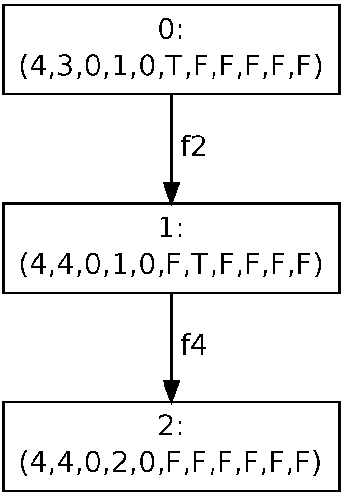
Examples of the risk propagation process are given in Figure 4 and Figure 5. The first part of the reachability graph (see Figure 4) represents the propagation of risk after firing transition . The starting point for that process is marking , where places are ordered as follows . The transition changes the value from 3 to 4 and sets the marking of trigger place to (T). The risk propagation contains two steps. First of all, a new risk value for component is evaluated and the marking of trigger place is set to . Then, a new risk value of component is evaluated that provides the stable marking denoted by 2 in the figure.
Suppose, the marking is the current marking and transition changes the value from 0 to 2 and sets the marking of trigger places , , , and to . We must propagate this change to all other components of the model. The part of the reachability graph shown in Figure 5 presents all possible paths that lead to the stable marking denoted by 19 in the figure. It is easy to observe that only few paths have length 4 i.e., each transition is fired at most once.
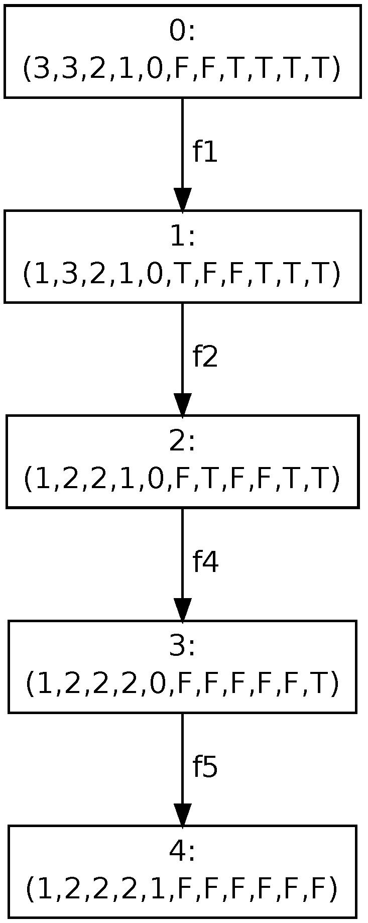
From the practical point of view, considering all possible paths of risk propagation is unnecessary. To reduce the presented part of the reachability graph transitions, priorities are used. Suppose the transitions have assigned priorities such as . If two transitions are enabled in the same marking and compete for the same place (or places), then the transition with the higher priority takes precedence over the second one. Thus, the risk propagation for component is reduced to the path shown in Figure 6.
At the end of this section, let us go back to the set of internal dependencies. It is possible to define symmetric dependencies between two functions , i.e., is an argument of and vice versa. Moreover, we say that functions are serially dependent if is an argument of , is an argument of , etc. and finally is an argument of . This may lead to an infinite propagation process i.e., an infinite sequence of transitions that does not lead to a stable marking.
6. Algorithm of Propagation Net Generation
A propagation net represents an algorithm of values propagation of the selected characteristic among components of the system under consideration. If propagation of more than one characteristic is necessary, an individual net should be constructed for each of them. For each characteristic, an individual set of internal dependencies is defined so two propagation nets constructed for the same system may differ about the set of trigger places.
Suppose the following items are given:
- the set of system components ;
- a characteristic ;
- the set of system border components , for which the value of the characteristic f may be modified directly due to some changes in the system environment;
- the set of internal dependencies F, where each function is assigned to the component and the value may be evaluated using values of the characteristic f for the system components only, .For a component , the symbol denotes the set of components that are necessary to evaluate i.e., values of the characteristic f for components from the set are necessary to evaluate .
The algorithm of propagation net generation is given in Algorithm 1. This is a formal description of the method described in Section 3. In case of the set A, a pair represents an arc going from x to y.
Propagation nets provide a formal model of the process of a risk or other system characteristic propagation. The model may be used to verify formally whether some required properties hold for the system or not. For example, we can check whether the net always reaches a stable marking.
| Algorithm 1 Algorithm of propagation net generation |
|
LTS graphs are universal methods for representation of a state space and are commonly used in formal modelling languages. Various formal languages like time automata, process algebras, Petri nets, etc. use different patterns of describing nodes and edges in LTS graphs. They also use different names and attributes for them e.g., reachability graphs in Petri nets, but the comprehensive structure of these graphs is still the same. In spite of the availability of dedicated tools designed for specific formalisms, there are also universal tools for verification of LTS graphs regardless of the formalism that is the source of such an LTS graph generation. Usually, such tools use model checking techniques for LTS graph verification [20].
In the presented approach, two verification scenarios using mainstream model checkers are considered—nuXmv for linear (LTL) and computation (CTL) temporal logics, and the Construction and Analysis of Distributed Processes (CADP) Evaluator for regular alternation-free μ-calculus.
The nuXmv tool [23] (the previous version known as NuSMV) is one of the most popular model checkers for temporal logic. Given a finite state model and a temporal logic formula, nuXmv can be used to check automatically whether the model satisfies the formula or not. Formulas can be perceived as requirements for the specific model and can be expressed using LTL [24] or CTL [24], temporal logics [25]. In the nuXmv approach, the verified system is modelled as a finite state transition system [26] usually called Kripke structure [27]. A method of translation of a Petri net reachability graph into the NuSMV language was proposed in [28]. The approach is rather states oriented i.e., logic formulas describe properties of reachable markings. Satisfaction of each specified formula is automatically verified with the nuXmv tool. If a modelled system does not satisfy a given formula, a proper counterexample is presented. It is also worth emphasizing that nuXmv can verify systems of high complexity, i.e., containing more than states.
The CADP toolbox [29] provides an action-oriented approach to LTS graph verification. One of the CADP tools called evaluator provides on-the-fly model checking of regular alternation-free μ-calculus formulas [30,31]. The μ-calculus formulas concern action labels and describe sequences of performed actions. The logic is built from three types of formulas: action, regular and state formulas. Action formulas deal with single steps (single arcs in an LTS graph), regular formulas represent regular expressions over action sequences, and, finally, state formulas represent properties of the considered system to be checked. Among other things, μ-calculus provides minimal and maximal fixed point operators. Intuitively, minimal (maximal) fixed point operators allow for characterizing finite (infinite) tree-like patterns in the LTS. Thus, we can check, for example, whether there is such a loop of transitions that a stable marking is never reached.
7. Proof of Concept Example
The presented method—as mentioned in the introduction—was proposed within realization of the project “Cyberspace Security Threats Evaluation System of the Republic of Poland”. The main achievements within realization of the project are [1]:
- the model of cyber threats,
- risk assessment of critical infrastructures’ assets and propagation of these risks among related elements,
- the model of the decision support subsystem for simulations of vulnerabilities’ exploitations,
- the method of emergency state attribution,
- the concept of information exchange between the agencies responsible for the cyberspace monitoring,
- implementation of the system for security evaluation of the Republic of Poland cyberspace.
The evaluation of risk for Polish cyber space includes (but is not limited to): energy and fuel supply systems, communication and IT network systems, banking and financial systems, food supply systems, water supply systems, health protection systems, transportation systems, etc.
The advantage of the proposed method is the assessment of the risk in three various cases:
- own—calculated with the use of factors typical for a particular component,
- static—assessed on the basis of relation of this node in the whole infrastructure and influence of cooperating or isomorphic components,
- dynamic—evaluated on the basis of current static risk and incoming security incident reports.
The method allows for distribution of any system feature, e.g., the three classic security pillars—Confidentiality, Integrity, and Availability. In such a way, we can estimate how security of one element of the infrastructure affects cooperating nodes and the whole network. Additionally, the method allows for verifying system security in cases of possible cyber attacks. This functionality can be used for system behaviour modelling as well as for verification of additional security measures adaptation for protecting the infrastructure or the particular node. On the basis of estimated levels of risk for particular elements and the propagation method, the administrator or user of the system can monitor the status of the risk and inform stakeholders about negative effects and possible changes (mitigation of the risk) after adaptation of security measures. Thus, ramifications can be modelled if some negative situations take place or additional protections are applied. Therefore, the proposed method supports decision makers in taking appropriate actions to protect monitored infrastructure.
8. Conclusions
This article presents the method of risk propagation proposed within the project Cyberspace Security Threats Evaluation System of the Republic of Poland. The advantage of this method is the possibility to model mutual impact on the cooperated and isomorphic components within the system. The method is formally described and the new class of propagation nets is defined. The proposed method can be used for various purposes, not only for assessing the risk in the cyber space or in critical infrastructures. The method was verified both in terms of its substantive correctness and for modelling and propagation of the risk.
Acknowledgments
This work has been partially supported by the Polish National Centre for Research and Development under the project “Cyberspace Security Threats Evaluation System of the Republic of Poland” No. DOBR-BIO4/011/13221/2013 and by the European Regional Development Fund of the Innovative Economy Operational Programme, under the project “Cyber Security Laboratory” No. 02.03.00-14-106/13. Cyberspace Security Threats Evaluation System of the Republic of Poland was developed by the consortium: Polish Military Communication Institute (leader) and Enamor International Ltd., Warsaw, Poland.
Author Contributions
Bartosz Jasiul and Marcin Szpyrka have equally contributed to the study and preparation of the article. All authors have read and approved the final manuscript.
Conflicts of Interest
The authors declare no conflict of interest. The founding sponsors had no role in the design of the study; in the collection, analyses, or interpretation of data; in the writing of the manuscript, and in the decision to publish the results.
Abbreviations
The following abbreviations are used in this manuscript:
| AGH | Akademia Górniczo-Hutnicza |
| CADP | Construction and Analysis of Distributed Processes |
| CI | Critical Infrastructure |
| CTL | Computation Temporal Logic |
| ISO/IEC | International Organization for Standardization/International Electrotechnical Commission |
| IT | Information Technology |
| LTL | Linear Temporal Logic |
| LTS | Labelled Transition System |
| NIST | National Institute of Standards and Technology |
| PMBoK | Project Management Body of Knowledge |
| SCADA | Supervisory Control and Data Acquisition |
| SP | Special Publication |
References
- Piotrowski, R.; Śliwa, J. Cyberspace Situational Awarness in National Security System. In Proceedings of the International Conference on Military Communications and Information Systems (ICMCIS), Cracow, Poland, 18–19 May 2015; pp. 1–6.
- ISO/IEC Information Technology. Security Techniques. Information Security Risk management, ISO/IEC 27005:2011; International Organization for Standardization: Geneva, Switzerland, 2011.
- Ross, R. Guide for Conducting Risk Assessments; National Institute of Standards and Technology: Gaithersburg, MA, USA, 2011. [Google Scholar]
- Sun, L.; Srivastava, R.; Mock, T. An Information Systems Security Risk Assessment Model Under the Dempster-Shafer Theory of Belief Functions. J. Manag. Inf. Syst. 2006, 22, 109–142. [Google Scholar] [CrossRef]
- Yi, T.; Lei, Y.; Chen, H.P.; Siamak, T.; Kang, F. Statistical and Probabilistic Approach in Monitoring-Based Structure Rating and Risk Assessment. Math. Probl. Eng. 2014, 2014, 761341. [Google Scholar] [CrossRef]
- Vrabel, R.; Abas, M.; Tanuska, P.; Vazan, P.; Kebisek, M.; Elias, M.; Sutova, Z.; Pavliak, D. Mathematical Approach to Security Risk Assessment. Math. Probl. Eng. 2015, 2015, 417597. [Google Scholar] [CrossRef]
- Cui, F.; Zhang, L.; Yu, C.; Hu, S.; Zhang, Y. Estimation of the Disease Burden Attributable to 11 Risk Factors in Hubei Province, China: A Comparative Risk Assessment. Int. J. Environ. Res. Public Health 2016, 13, 944. [Google Scholar] [CrossRef] [PubMed]
- He, Y.; Peng, S.; Xiong, W.; Xu, Y.; Liu, J. Association between Polymorphism of Interleukin-1beta and Interleukin-1 Receptor Antagonist Gene and Asthma Risk: A Meta-Analysis. Sci. World J. 2015, 2015, 685684. [Google Scholar] [CrossRef] [PubMed]
- Farooq, A.; Naveed, A.; Azeem, Z.; Ahmad, T. Breast and Ovarian Cancer Risk due to Prevalence of BRCA1 and BRCA2 Variants in Pakistani Population: A Pakistani Database Report. J. Oncol. 2011, 2011, 632870. [Google Scholar] [CrossRef] [PubMed]
- Quan, G. Performance and Risk Assessment of Soil-Structure Interaction Systems Based on Finite Element Reliability Methods. Math. Probl. Eng. 2014, 2014, 704804. [Google Scholar]
- Serra-Llobet, A.; Conrad, E.; Schaefer, K. Governing for Integrated Water and Flood Risk Management: Comparing Top-Down and Bottom-Up Approaches in Spain and California. Water 2016, 8, 445. [Google Scholar] [CrossRef]
- Szpyrka, M.; Jasiul, B.; Wrona, K.; Dziedzic, F. Telecommunications Networks Risk Assessment with Bayesian Networks. In Computer Information Systems and Industrial Management, Proceedings of the 12th IFIP TC8 International Conference CISIM 2013, Krakow, Poland, 25–27 September 2013; Saeed, K., Chaki, R., Cortesi, A., Wierzchoń, S., Eds.; Springer: Berlin, Germany, 2013; Volume 8104, pp. 277–288. [Google Scholar]
- Garrido, A. Essential Graphs and Bayesian Networks. In Proceedings of the First International Conference on Complexity and Intelligence of the Artificial and Natural Complex Systems, Medical Applications of the Complex Systems, Biomedical Computing (CANS’08), Tirgu Mures, Romania, 8–10 November 2008; IEEE: Piscataway, NJ, USA, 2008; pp. 149–156. [Google Scholar]
- Schneier, B. Attack Trees. Dr Dobb’s J. 1999, 24, 21–29. [Google Scholar]
- Szwed, P.; Skrzynski, P.; Chmiel, W. Risk assessment for a video surveillance system based on Fuzzy Cognitive Maps. Multimed. Tools Appl. 2016, 75, 10667–10690. [Google Scholar] [CrossRef]
- Henry, M.H.; Layer, R.M.; Snow, K.Z.; Zaret, D.R. Evaluating the risk of cyber attacks on SCADA systems via Petri net analysis with application to hazardous liquid loading operations. In Proceedings of the 2009 IEEE Conference on Technologies for Homeland Security, Waltham, MA, USA, 11–12 May 2009; pp. 607–614.
- Jensen, K.; Kristensen, L. Coloured Petri Nets. Modelling and Validation of Concurrent Systems; Springer: Heidelberg, Germany, 2009. [Google Scholar]
- Jasiul, B.; Szpyrka, M.; Śliwa, J. Detection and Modeling of Cyber Attacks with Petri Nets. Entropy 2014, 16, 6602–6623. [Google Scholar] [CrossRef]
- Szpyrka, M. Analysis of RTCP-nets with Reachability Graphs. Fundam. Inform. 2006, 74, 375–390. [Google Scholar]
- Baier, C.; Katoen, J.P. Principles of Model Checking; The MIT Press: London, UK, 2008. [Google Scholar]
- O’Sullivan, B.; Goerzen, J.; Stewart, D. Real World Haskell; O’Reilly Media: Sebastopol, CA, USA, 2008. [Google Scholar]
- Gansner, E.; Koutsofios, E.; North, S. Drawing Graphs with Dot. Available online: http://graphviz.org/Documentation/dotguide.pdf (accessed on 23 February 2017).
- Cavada, R.; Cimatti, A.; Dorigatti, M.; Griggio, A.; Mariotti, A.; Micheli, A.; Mover, S.; Roveri, M.; Tonetta, S. The nuXmv Symbolic Model Checker. In Computer Aided Verification; Lecture Notes in Computer Science; Springer: Berlin, Germany, 2014; Volume 8559, pp. 334–342. [Google Scholar]
- Clarke, E.; Grumberg, O.; Peled, D. Model Checking; The MIT Press: Cambridge, MA, USA, 1999. [Google Scholar]
- Emerson, E. Temporal and modal logic. In Handbook of Theoretical Computer Science; van Leeuwen, J., Ed.; Elsevier Science: Amsterdam, the Netherlands, 1990; Volume B, pp. 995–1072. [Google Scholar]
- Cimatti, A.; Clarke, E.; Giunchiglia, F.; Roveri, M. NUSMV: A new symbolic model checker. Int. J. Softw. Tools Technol. Transf. 2000, 2, 410–425. [Google Scholar] [CrossRef]
- Kripke, S. A semantical analysis of modal logic I: Normal modal propositional calculi. Z. Math. Logik und Grundlagen der Math. 1963, 9, 67–96. [Google Scholar] [CrossRef]
- Szpyrka, M.; Biernacki, J.; Biernacka, A. Tools and methods for RTCP-nets modelling and verification. Arch. Control Sci. 2016, 26, 339–365. [Google Scholar]
- Garavel, H.; Lang, F.; Mateescu, R.; Serwe, W. CADP 2006: A Toolbox for the Construction and Analysis of Distributed Processes. In Computer Aided Verification; Springer: Berlin, Germany, 2007; Volume 4590, pp. 158–163. [Google Scholar]
- Emerson, E. Model checking and the Mu-Calculus; DIMACS Series in Discrete Mathematics; American Mathematical Society: Providence, RI, USA, 1997; pp. 185–214. [Google Scholar]
- Mateescu, R.; Sighireanu, M. Efficient On-the-Fly Model-Checking for Regular Alternation-Free μ-Calculus; Technical Report 3899; INRIA: Rocquencourt, France, 2000. [Google Scholar]
Figure 1.
Part of the propagation net for representation of function .

Figure 2.
Part of the propagation net for representation of transition .
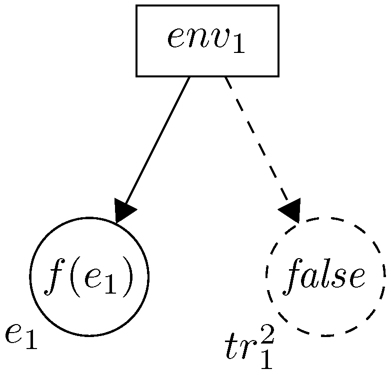
Figure 3.
Propagation net.
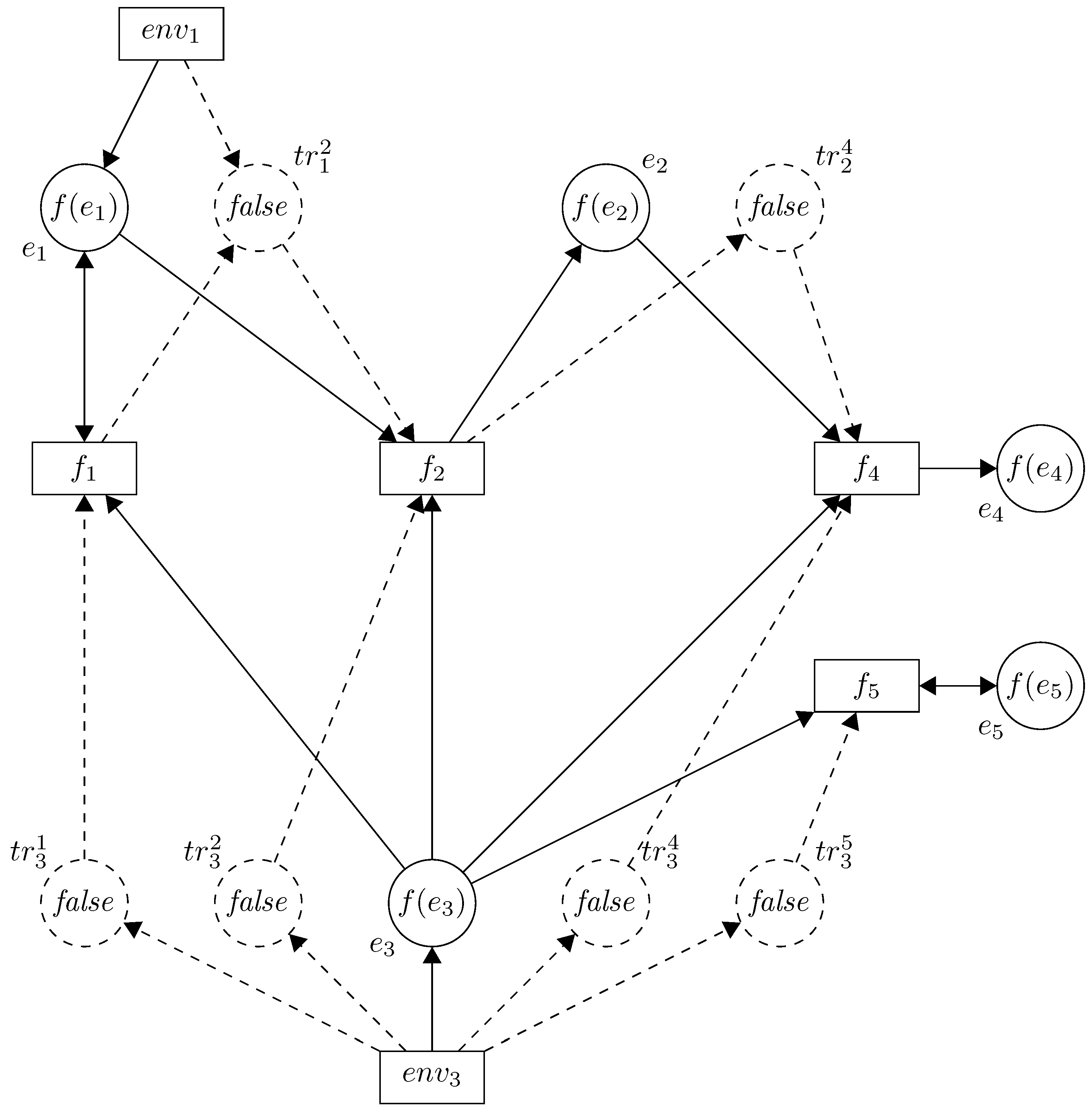
Figure 4.
Risk propagation for component .

Figure 5.
Risk propagation for component .
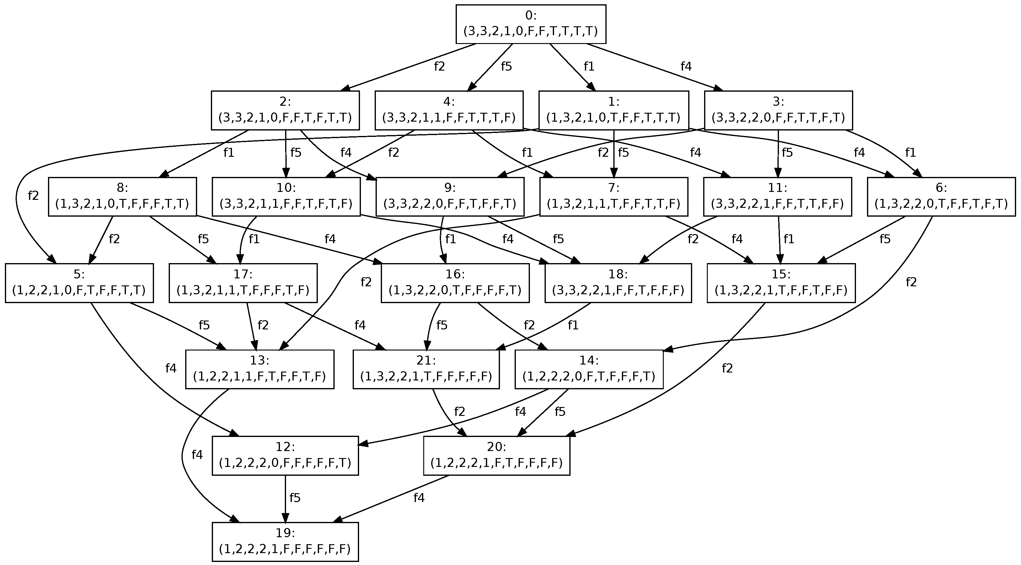
Figure 6.
Risk propagation for component —with priorities.

| × | × | ||||
| × | × | ||||
| × | × | ||||
| × | × |
© 2017 by the authors. Licensee MDPI, Basel, Switzerland. This article is an open access article distributed under the terms and conditions of the Creative Commons Attribution (CC BY) license ( http://creativecommons.org/licenses/by/4.0/).
Share and Cite
MDPI and ACS Style
Szpyrka, M.; Jasiul, B. Evaluation of Cyber Security and Modelling of Risk Propagation with Petri Nets. Symmetry 2017, 9, 32. https://doi.org/10.3390/sym9030032
AMA Style
Szpyrka M, Jasiul B. Evaluation of Cyber Security and Modelling of Risk Propagation with Petri Nets. Symmetry. 2017; 9(3):32. https://doi.org/10.3390/sym9030032
Chicago/Turabian StyleSzpyrka, Marcin, and Bartosz Jasiul. 2017. "Evaluation of Cyber Security and Modelling of Risk Propagation with Petri Nets" Symmetry 9, no. 3: 32. https://doi.org/10.3390/sym9030032
Note that from the first issue of 2016, this journal uses article numbers instead of page numbers. See further details here.