Solving Solar-Wind Power Station Location Problem Using an Extended Weighted Aggregated Sum Product Assessment (WASPAS) Technique with Interval Neutrosophic Sets

Abstract

As one of the promising renewable energy resources, solar-wind energy has increasingly become a regional engine in leading the economy and raising competitiveness. Selecting a solar-wind power station location can contribute to efficient utilization of resource and instruct long-term development of socio-economy. Since the selection procedure consists of several location alternatives and many influential criteria factors, the selection can be recognized as a multiple criteria decision-making (MCDM) problem. To better express multiple uncertainty information during the selection procedure, fuzzy set theory is introduced to manage that issue. Interval neutrosophic sets (INSs), which are characterized by truth-membership, indeterminacy-membership and falsity-membership functions in the interval numbers (INs) form, are feasible in modeling more uncertainty of reality. In this paper, a newly extended weighted aggregated sum product assessment (WASPAS) technique, which involves novel three procedures, is utilized to handle MCDM issues under INSs environment. Some modifications are conducted in the extended method comparing with the classical WASPAS method. The most obvious improvement of the extended method relies on that it can generate more realistic criteria weight information by an objective and subjective integrated criteria weight determination method. A case study concerning solar-wind power station location selection is implemented to demonstrate the applicability and rationality of the proposed method in practice. Its validity and feasibility are further verified by a sensitivity analysis and a comparative analysis. These analyses effectively reveal that the extended WASPAS technique can well match the reality and appropriately handle the solar-wind power station location selection problem.

1. Introduction

Remarkable growth of urbanization and industrialization make it imperative to increase widespread useable electricity for facilitating regional economy development [1]. Due to the increasing awareness of the global climate degradation, conventional energy resources cannot simultaneously meet the environmental challenge and energy demand [2]. The solar-wind energy system has gradually substituted the status of traditional energy for the friendly environment concern [3]. Solar-wind power station devotes to convert renewable resources such as solar and wind energy into power for supporting socio-economic requirement [4]. For better contributing to regional competition and determining future energy generation, it is significant to seek a good solar-wind power station location [5]. Considerable researches have increasingly emerged concerning selecting the renewable energy location [6]. It is well known that the usage starting point of multiple criteria decision analysis (MCDA) is a definition of the set of decision variants [7]. The aim of MCDA is to select a good solution according to decision makers’ (DMs’) preferences [8,9]. As numerous influential factors need to be considered in the selecting procedure, the location selection problem can be treated as a complex multiple criteria decision-making (MCDM) problem [6]. In addition, MCDM methods have been adopted as effective instruments in this field. Incorporating analytic hierarchy process (AHP) to GIS environment, the most desirable nuclear power plant location was determined by MCDM analysis technique [10]. The framework of MCDM analysis based on GIS was also identified as an effective decision tool for wind-farm location planning area [11]. Furthermore, grey cumulative prospect theory and cloud decision framework were gradually employed into power location selection [12,13]. To manage inevitable fuzziness and uncertainty in realistic application, ELECTRE-III as one of the most commonly used MCDM technique was extended into intuitionistic fuzzy circumstances for determining a good offshore wind power station location [14]. The selection of the solar-wind power station location can be regarded as another complex MCDM problem involving many influential factors such as economic factors, traffic factors, natural resources, environmental factors and social factors [15]. Though MCDM methods such as ELECTRE-II has been widely employed into this field [15], existing researches concerning solar-wind power station location selection neglect the impact of uncertainty and only evaluate the alternatives in the real number context [16]. Effective information expression form should be introduced into the selection problem for representing more abundant and realistic information.

Along with the development of fuzzy set theory, fuzzy set (FSs) [17] as well as interval valued fuzzy sets (IVFSs) [18], intuitionistic fuzzy sets [19] and interval-valued intuitionistic fuzzy sets (IVIFSs) [20] were extensively applied into dealing with uncertain situation. Owing to multiple uncertainty and information existing in practice, above traditional types of FSs are unable to adequately express indeterminate information and inconsistent information [21]. Neutrosophic sets (NSs) [22] were initially presented by Smarandache to feasibly manage these uncertain information via considering the truth membership, indeterminacy membership and falsity membership functions simultaneously [23,24]. However, NS was lacking of specific description to adequately express actual issues. As a particular case of NSs, single-valued neutrosophic sets (SVNSs) were introduced for the first time by Smarandache in 1998 in his book [22], reviewed in [25], which is also mentioned by Denis Howe, from England, in The Free Online Dictionary of Computing, 1999. Since more information can be described by interval numbers (INs), interval neutrosophic set (INS) [26] as a further extension of NS was utilized in various fields such as trustworthy cloud service selection [27], lean supplier selection [28] and medical diagnosis [29]. Relative basic theories of INS which briefly focus on its aggregation operators and MCDM methods have already developed maturity [30]. Particularly, MCDM methods including outranking approach [31], cross-entropy measure [32], and correlation coefficient measure [33] can effectively deal with problems under INS environment. This paper aims to develop a novel MCDM technique with flexibility and applicability under INSs circumstances for matching the solar-wind power station location selection case.

The weighted aggregated sum product assessment (WASPAS) method was originally presented in 2012 regarded as an effective extension of Weighted Product Model (WPM) and Weighted Sum Model (WSM) [34]. Its accuracy in dealing with MCDM problems has been proven by comparing with the simple utilization one of WPM or WSM [34]. This method has been extensively employed into MCDM situation and various applications [35], especially in the site selection field. The complex circuit design of lead-zinc froth flotation selection regarded as a MCDM procedure was adequately settled by WASPAS method for fully processing costs and reinforcing the utilization [36]. Selection of the best wind farm location was feasibly handled and assessed by utilizing the WASPAS method [37]. The selection of the construction site for a waste incineration plant plays a critical role in public health and city development. It can be effectively solved by means of the WASPAS method [38]. Within the MCDM framework, relevant mathematical model and AHP approach were incorporated into the WASPAS method, by which the location selection problem of the garage was explicitly formulated [39]. Its robustness was verified by comparing with other MCDM methods when finding a good solution [40]. Referring to specific application setting, WASPAS method has been generalized into a variety of assessment fields such as energy supply system [41], solar projects [42], third-party logistics providers [43] and indoor environment [35]. The combination of the WASPAS method with fuzzy set theory has been introduced into dealing with uncertainty under grey values [44], interval type-2 fuzzy sets [43] or SVNSs environment [45]. Incorporating IVIFSs into WASPAS method, it can effectively deal with the MCDM problems [46]. Relative research concerning the WASPAS technique with INSs needs to be further investigated to enrich theory basics and represent more uncertain information. Consequently, this paper generalizes the WASPAS technique into INSs circumstances for matching the solar-wind power station location selection problem.

Previous researches have revealed that incomplete or unknown weight information commonly exists when applying the MCDM methods into assessment [47]. From the perspective of the objective weight determination methods, maximizing derivation method [48], the most widely utilized method, can generate the criteria weights under weights partly known or completely unknown circumstances. Corresponding mathematical programming models are constructed according to different circumstances such as hesitant fuzzy sets [49,50], IFSs [51] and multiple types of linguistic circumstances [52,53]. As one of the representative subjective weight determination methods, order relation analysis method (G1) determines the weight information by virtue of DMs’ experience judgement [54]. G1 not only reflects the subjective judgment of DMs, but also possesses convenience and feasibility comparing to AHP method. These advantages are due to its simple acquisition process, and the fact that there is no need to construct judgement matrix [54]. To adequately reflect more realistic information from both the subjective and objective aspects, this paper investigates an integrated criteria weight utilizing the combination strengths of above determination methods, and further employs it to the WASPAS technique under INSs environment.

The reminder of the paper is structured as follows. In Section 2, some basic concepts concerning INs and INSs are roughly reviewed. In Section 3, the framework of the extended WASPAS technique is constructed based on the objective weight and subjective weight integrated criteria weight information. Subsequently, to verify its applicability within INSs environment, the extended WASPAS technique is employed into practical solar-wind power station location case in Section 4. In Section 5, a sensitivity analysis and a comparative analysis are conducted to further demonstrate the rationality of the extended WASPAS technique. Finally, conclusions are summarized in Section 6.

2. Background

This section briefly reviews some basics concerning INSs for the latter discussion.

2.1. INs

Some definitions and concepts of INs are recalled.

Definition 1.

[55] Let $a=\left[a^L,a^U\right]=\left\{x|a^L\le x\le a^U\right\}$, then $a$ is said to be an IN. Particularly, $a=\left[a^L,a^U\right]$ will be deduced to a real number if $a^L=a^U$.

Assume that there are two nonnegative INs $a_1=\left[a_1^L,a_1^U\right]$ and $a_2=\left[a_2^L,a_2^U\right]$. Then, their operations are defined as follows [56]:

• $a_1+a_2=\left[a_1^L+a_2^L,a_1^U+a_2^U\right]$,
• $\lambda a_1=\left[\lambda a_1^L,\lambda a_1^U\right],\lambda >0.$

Definition 2.

[30] Let $a_1=\left[a_1^L,a_1^U\right]$ and $a_2=\left[a_2^L,a_2^U\right]$ be two INs, $L\left(a_1\right)=a_1^u-a_1^L$ and $L\left(a_2\right)=a_2^u-a_2^L$, then the possibility degree of $a_1\ge a_2$ is denoted as:

$$p\left(a_1\ge a_2\right)=\max \left\{1-\max \left\{\frac{a_2^U-a_1^L}{L\left(a_1\right)+L\left(a_2\right)},0\right\},0\right\},$$

(1)

Consider there exist $m$ INs $a_i=\left[a_i^L,a_i^U\right]$ $\left(i=1,2,\dots ,m\right)$. The possibility degree of Equation (1) can be denoted as

$$p\left(a_i\ge a_j\right)=\max \left\{1-\max \left\{\frac{a_j^U-a_i^L}{L\left(a_i\right)+L\left(a_j\right)},0\right\},0\right\},$$

(2)

when comparing each IN $a_i$ to all INs $a_j=\left[a_j^L,a_j^U\right]$$\left(j=1,2,\dots ,n\right)$. Then, a complementary possibility degree matrix can be established as

$$P\left(a_i\ge a_j\right)={\left[\begin{array}{cccc}{p}_{11}& p_{12}& \dots & p_{1n}\\ p_{21}& p_{22}& \dots & p_{2n}\\ & & ⋮& \\ p_{n1}& p_{n2}& \dots & p_{nn}\end{array}\right]}_{n\times n},$$

(3)

whose elements satisfy the conditions $p_{ij}\ge 0$, $p_{ij}+p_{ji}=1$ and $p_{ii}=0.5$. Its ranking vector can be derived from the equation as follows:

$$p_i=\frac{{\displaystyle \sum _{j=1}^n{p}_{ij}+\frac{m}{2}-1}}{m\left(m-1\right)},\left(i=1,2,\dots ,m\right),$$

(4)

2.2. INSs

Due to the fact that indeterminacy and inconsistency information commonly exist in the daily life, numerous researches tackled the NSs as the instrument to manage that issue [57,58]. However, to fully and adequately indicate uncertainty and fuzziness in the reality, IN is utilized as the form to depict the truth-membership, indeterminacy-membership and falsity-membership information of NSs rather than crisp values [59]. In this section, we briefly review some basics of INSs, which involves operational laws, aggregation operators and score functions. For the convenience of expressing the reality, INS is defined motivated by the definition of SVNS as follows:

Definition 3.

[60] Let $X$ be an arbitrary universe of discourse whose generic element can be denoted by $x$. Then, an INS $A$ in $X$ is

$$A=\left\{\langle x,T_A\left(x\right),I_A\left(x\right),F_A\left(x\right)\rangle |x\in X\right\},$$

(5)

which is characterized by a truth-membership function $T_A\left(x\right)$, an indeterminacy-membership function $I_A\left(x\right)$ and a falsity-membership function $F_A\left(x\right)$. For each point of $x$ in $X$, there exists the conditions that $T_A\left(x\right)=\left[T_A^L\left(x\right),T_A^U\left(x\right)\right]$, $I_A\left(x\right)=\left[I_A^L\left(x\right),I_A^U\left(x\right)\right]$, $F_A\left(x\right)=\left[F_A^L\left(x\right),F_A^U\left(x\right)\right]$ and $T_A\left(x\right),I_A\left(x\right),F_A\left(x\right)\subseteq \left[0,1\right]$ and $0\le T_A^U\left(x\right)+I_A^U\left(x\right)+F_A^U\left(x\right)\le 3$.

For notation simplification, we adopt $a=\langle \left[T^L,T^U\right],\left[I^L,I^U\right],\left[F^L,F^U\right]\rangle$ as the representation of an INS in this paper.

Definition 4.

[61] Let $a_1=\langle \left[T_1^L,T_1^U\right],\left[I_1^L,I_1^U\right],\left[F_1^L,F_1^U\right]\rangle$ and $a_2=\langle \left[T_2^L,T_2^U\right],\left[I_2^L,I_2^U\right],\left[F_2^L,F_2^U\right]\rangle$ be two arbitrary INSs, then, its operational laws can be defined as

(1) 

The complement of $a_1$ is ${\overline{a}}_1=\langle \left[F_1^L,F_1^U\right],\left[1-I_1^U,1-I_1^L\right],\left[T_1^L,T_1^U\right]\rangle$,

(2) 

$a_1+a_2=\langle \left[T_1^L+T_2^L-T_1^L{T}_2^L,T_1^U+T_2^U-T_1^U{T}_2^U\right],\left[I_1^L{I}_2^L,I_1^U{I}_2^U\right],\left[F_1^L{F}_2^L,F_1^U{F}_2^U\right]\rangle ,$

(3) 

$a_1\times a_2=\begin{array}{c}\langle \left[T_1^L{T}_2^L,T_1^U{T}_2^U\right],\left[I_1^L+I_2^L-I_1^L{I}_2^L,I_1^U+I_2^U-I_1^U{I}_2^U\right],\hfill \\ \left[F_1^L+F_2^L-F_1^L{F}_2^L,F_1^U+F_2^U-F_1^U{F}_2^U\right]\rangle ,\hfill \end{array}$

(4) 

$\eta a_1=\langle \left[1-{\left(1-T_1^L\right)}^{\eta },1-{\left(1-T_1^U\right)}^{\eta }\right],\left[{\left(I_1^L\right)}^{\eta },{\left(I_1^U\right)}^{\eta }\right],\left[{\left(F_1^L\right)}^{\eta },{\left(F_1^U\right)}^{\eta }\right]\rangle ,\eta >0$,

(5) 

${a_1}^{\eta }=\langle \left[{\left(T_1^L\right)}^{\eta },{\left(T_1^U\right)}^{\eta }\right],\left[1-{\left(1-I_1^L\right)}^{\eta },1-{\left(1-I_1^U\right)}^{\eta }\right],\left[1-{\left(1-F_1^L\right)}^{\eta },1-{\left(1-F_1^U\right)}^{\eta }\right]\rangle ,\eta >0.$

Definition 5.

[61] Let $a_j=\langle \left[T_j^L,T_j^U\right],\left[I_j^L,I_j^U\right],\left[F_j^L,F_j^U\right]\rangle$ $\left(j=1,2,\dots ,n\right)$ be a permutation of the INSs. Then, the interval neutrosophic power generalized weighted aggregation operator is defined as

$$INPGWA\left(a_1,a_2,\cdots ,a_n\right)={\left({\displaystyle \sum _{j=1}^n\frac{{\omega }_j\left(1+T\left(a_j\right)\right){a_j}^{\eta }}{{\displaystyle \sum _{j=1}^n{\omega }_j\left(1+T\left(a_j\right)\right)}}}\right)}^{1/\eta },$$

(6)

in which ${\omega }_j=\left({\omega }_1,{\omega }_2,\cdots ,{\omega }_n\right)$ is the associated weight vector of $a_j$$\left(j=1,2,\dots ,n\right)$, ${\omega }_j\in \left[0,1\right]$, ${\displaystyle \sum _{j=1}^n{\omega }_j=1}$; $T\left(a_j\right)={\displaystyle \sum _{\begin{array}{l}i=1,\\ i\ne j\end{array}}^{n}Sup\left(a_j,a_i\right)}$, $Sup\left(a_j,a_i\right)$ is the support degree for $a_j$ from $a_i$; $\eta$ is a parameter belonging to $\left(0,+\infty \right)$.

Theorem 1.

[61] Let $a_j=\langle \left[T_j^L,T_j^U\right],\left[I_j^L,I_j^U\right],\left[F_j^L,F_j^U\right]\rangle$ $\left(j=1,2,\dots ,n\right)$ be a permutation of the INSs, the aggregated result utilizing the interval neutrosophic power generalized weighted aggregation operator derived from Definition 4 is shown as

$$\begin{array}{cc}\hfill INPGWA\left(a_1,a_2,\cdots ,a_n\right)=& \langle \left[{\left(1-{\displaystyle \prod _{j=1}^n{\left(1-{\left(T_j^L\right)}^{\eta }\right)}^{w_j}}\right)}^{1/\eta },{\left(1-{\displaystyle \prod _{j=1}^n{\left(1-{\left(T_j^U\right)}^{\eta }\right)}^{w_j}}\right)}^{1/\eta }\right],\hfill \\ & \left[1-{\left(1-{\displaystyle \prod _{j=1}^n{\left(1-{\left(I_j^L\right)}^{\eta }\right)}^{w_j}}\right)}^{1/\eta },1-{\left(1-{\displaystyle \prod _{j=1}^n{\left(1-{\left(I_j^U\right)}^{\eta }\right)}^{w_j}}\right)}^{1/\eta }\right],\hfill \\ & \left[1-{\left(1-{\displaystyle \prod _{j=1}^n{\left(1-{\left(F_j^L\right)}^{\eta }\right)}^{w_j}}\right)}^{1/\eta },1-{\left(1-{\displaystyle \prod _{j=1}^n{\left(1-{\left(F_j^U\right)}^{\eta }\right)}^{w_j}}\right)}^{1/\eta }\right]\rangle ,\hfill \end{array}$$

(7)

in which $w_j=\frac{{\omega }_j\left(1+T\left(a_j\right)\right)}{{\displaystyle \sum _{j=1}^n{\omega }_j\left(1+T\left(a_j\right)\right)}}$. Particularly, when$\eta \to 0$, the interval neutrosophic power generalized weighted aggregation operator reduces to an interval neutrosophic power geometric weighted aggregation (INPGWA) operator, which is shown as

$$\begin{array}{cc}\hfill INPGWA\left(a_1,a_2,\cdots ,a_n\right)=& \langle \left[{\displaystyle \prod _{j=1}^n{\left(T_j^L\right)}^{w_j}},{\displaystyle \prod _{j=1}^n{\left(T_j^U\right)}^{w_j}}\right],\left[1-{\displaystyle \prod _{j=1}^n{\left(1-I_j^L\right)}^{w_j}},1-{\displaystyle \prod _{j=1}^n{\left(1-I_j^U\right)}^{w_j}}\right],\hfill \\ & \left[1-{\displaystyle \prod _{j=1}^n{\left(1-F_j^L\right)}^{w_j}},1-{\displaystyle \prod _{j=1}^n{\left(1-F_j^U\right)}^{w_j}}\right]\rangle ;\hfill \end{array}$$

(8)

When $\eta \to 1$, the interval neutrosophic power generalized weighted aggregation operator reduces to an interval neutrosophic power weighted aggregation (INPWA) operator, which is shown as

$$\begin{array}{cc}\hfill INPWA\left(a_1,a_2,\cdots ,a_n\right)=& \langle \left[1-{\displaystyle \prod _{j=1}^n{\left(1-T_j^L\right)}^{w_j}},1-{\displaystyle \prod _{j=1}^n{\left(1-T_j^U\right)}^{w_j}}\right],\hfill \\ & \hfill \left[{\displaystyle \prod _{j=1}^n{\left(I_j^L\right)}^{w_j}},{\displaystyle \prod _{j=1}^n{\left(I_j^U\right)}^{w_j}}\right],\left[{\displaystyle \prod _{j=1}^n{\left(F_j^L\right)}^{w_j}},{\displaystyle \prod _{j=1}^n{\left(F_j^U\right)}^{w_j}}\right]\rangle .\end{array}$$

(9)

Definition 6.

[62] Let $a_1=\langle \left[T_1^L,T_1^U\right],\left[I_1^L,I_1^U\right],\left[F_1^L,F_1^U\right]\rangle$ and $a_2=\langle \left[T_2^L,T_2^U\right],\left[I_2^L,I_2^U\right],\left[F_2^L,F_2^U\right]\rangle$ be two arbitrary INSs. Then, the normalized Hamming distance between $a_1$ and $a_2$ can be defined as

$$d\left(a_1,a_2\right)=\frac{1}{6}(\left|T_1^L-T_2^L\right|+\left|T_1^U-T_2^U\right|+\left|I_1^L-I_2^L\right|+\left|I_1^U-I_2^U\right|+\left|F_1^L-F_2^L\right|+\left|F_1^U-F_2^U\right|).$$

(10)

Definition 7.

[63] Let $a=\langle \left[T^L,T^U\right],\left[I^L,I^U\right],\left[F^L,F^U\right]\rangle$ be an INS, then, its score function as well as accuracy function and certainty function are defined as

(1)

$S\left(a\right)=\left[T^L+1-I^U+1-F^U,T^U+1-I^L+1-F^L\right],$

(2)

$H\left(a\right)=\left[\min \left\{T^L-F^L,T^U-F^U\right\},\max \left\{T^L-F^L,T^U-F^U\right\}\right],$

(3)

$B\left(a\right)=\left[T^L,T^U\right].$

Its comparison rules are specifically introduced in [63].

3. The Framework of an Extended WASPAS Technique

In this section, an extended WASPAS technique is newly investigated to match solar-wind power station location selection issue with completely unknown criteria weight information.

3.1. Maximizing Deviation Method for Objective Weight Estimating

The maximizing deviation method was initially presented by Wang [64] for managing MCDM problems in numerical context. Its main ideal relies on the performance value of each alternative differs under certain criteria. Thus, it can be inferred that if certain criteria makes the performance values concerning all the alternatives apparently different, the criteria plays a critical role in seeking a good alternative under the MCDM context. Therefore, by virtue of this ideal, criteria with similar performance value with respect to all the alternatives should be allocated small weight; otherwise, the criteria makes huge differences over alternatives should be allocated bigger weight. By above analysis, the maximizing deviation method can be applied into specific MCDM application as an effective tool in deriving completely unknown criteria weight information. Specially, the model, which reveals the differences of the performance value for each alternative, can be established in the following within the INS context.

With respect to certain criteria $C_j\in C$, the performance derivation values of alternative $x_i$ to all the other alternatives can be established as follows:

$$D_{ij}\left({\omega }^{\prime }\right)={\displaystyle \sum _{k=1}^{m}d\left(a_{ij},a_{kj}\right)}{\omega }_j^{\prime },i=1,2,\cdots ,m,j=1,2,\cdots ,n$$

(11)

in which $a_{ij}$ and $a_{kj}$ represent the performance value of alternative $i$ and alternative $k$ under criteria $j$, and characterized by $a_{ij}=\langle \left[T_{ij}^L,T_{ij}^U\right],\left[I_{ij}^L,I_{ij}^U\right],\left[F_{ij}^L,F_{ij}^U\right]\rangle$ and $a_{kj}=\langle \left[T_{kj}^L,T_{kj}^U\right],\left[I_{kj}^L,I_{kj}^U\right],\left[F_{kj}^L,F_{kj}^U\right]\rangle$, respectively.

Furthermore, let

$$D_j\left({\omega }^{\prime }\right)={\displaystyle \sum _{i=1}^m{D}_{ij}\left({\omega }^{\prime }\right)}={\displaystyle \sum _{i=1}^m{\displaystyle \sum _{k=1}^{m}d\left(a_{ij},a_{kj}\right)}{\omega }_j^{\prime }}$$

(12)

$D_j\left(\omega \right)$ represents the derivation performance value of all the alternatives to the others under criteria $C_j\in C$.

From above analysis, the determination of weight vector ${\omega }^{\prime }$ can maximize the collective derivation performance value for all the criteria. A linear programming model can be established to derive the optimal weight vector solution ${\omega }^{\prime }=\left({\omega }_1^{\prime },{\omega }_2^{\prime },\cdots ,{\omega }_n^{\prime }\right)$ which is utilized as the criteria weight vector, shown as follows:

$$\{\begin{array}{l}\max D\left({\omega }^{\prime }\right)={\displaystyle \sum _{j=1}^n{\displaystyle \sum _{i=1}^m{D}_{ij}\left({\omega }^{\prime }\right)}}={\displaystyle \sum _{j=1}^n{\displaystyle \sum _{i=1}^m{\displaystyle \sum _{k=1}^{m}d\left(a_{ij},a_{kj}\right)}{\omega }_j^{\prime }}}\\ s.t.{\omega }^{\prime }\in \mathsf{\Omega },{\displaystyle \sum _{j=1}^n{\omega }_j^{\prime }=1,{\omega }_j^{\prime }\ge 0,j=1,2,\cdots ,n,}\end{array}$$

(13)

in which specific distance equation $d\left(a_{ij},a_{kj}\right)$ refers to Definition 6. Above model is designed to solve the decision-making problem with partial known criteria weight information in $\mathsf{\Omega }$. However, due to the complexity in practice, criteria weight information tends to be completely unknown, and cannot be predefined in MCDM problems in most cases. Another programming model is established in the following to derive the criteria weight vector within the completely unknown weight information.

$$\{\begin{array}{l}\max D\left({\omega }^{\prime }\right)\\ ={\displaystyle \sum _{i=1}^m{D}_i\left({\omega }^{\prime }\right)}\\ =\frac{1}{6}{\displaystyle \sum _{j=1}^n{\displaystyle \sum _{i=1}^m{\displaystyle \sum _{k=1}^m(\left|T_{ij}^L-T_{kj}^L\right|+\left|T_{ij}^U-T_{kj}^U\right|+\left|I_{ij}^L-I_{kj}^L\right|+\left|I_{ij}^U-I_{kj}^U\right|+\left|F_{ij}^L-F_{kj}^L\right|+\left|F_{ij}^U-F_{kj}^U\right|)}{\omega }_j^{\prime }}}\\ s.t.{\displaystyle \sum _{j=1}^n{\left({\omega }_j^{\prime }\right)}^2=1,{{\omega }^{\prime }}_j\ge 0,j=1,2,\cdots ,n.}\end{array}$$

(14)

A Lagrange function can be established to solve this model, and shown as

$$\begin{array}{cc}\hfill L\left({\omega }^{\prime },\gamma \right)=\frac{1}{6}{\displaystyle \sum _{j=1}^n}{\displaystyle \sum _{i=1}^m}{\displaystyle \sum _{k=1}^m}& (\left|T_{ij}^L-T_{kj}^L\right|+\left|T_{ij}^U-T_{kj}^U\right|+\left|I_{ij}^L-I_{kj}^L\right|+\left|I_{ij}^U-I_{kj}^U\right|\hfill \\ & +\left|F_{ij}^L-F_{kj}^L\right|+\left|F_{ij}^U-F_{kj}^U\right|){\omega }_j^{\prime }+\frac{\gamma }{12}\left({\displaystyle \sum _{j=1}^n{\left({\omega }_j^{\prime }\right)}^2-1}\right),\hfill \end{array}$$

(15)

in which $\gamma$ is the Lagrange multiplier. Differentiating Equation (15) concerning ${\omega }_j^{\prime }$ $\left(j=1,2,\dots ,n\right)$ and $\gamma$, respectively. Let these partial derivations equal to 0 value, these equations can be derived as follows:

$$\{\begin{array}{l}\frac{\partial L}{\partial {\omega }_j^{\prime }}={\displaystyle \sum _{j=1}^n{\displaystyle \sum _{i=1}^m{\displaystyle \sum _{k=1}^m(\left|T_{ij}^L-T_{kj}^L\right|+\left|T_{ij}^U-T_{kj}^U\right|+\left|I_{ij}^L-I_{kj}^L\right|+\left|I_{ij}^U-I_{kj}^U\right|+\left|F_{ij}^L-F_{kj}^L\right|+\left|F_{ij}^U-F_{kj}^U\right|)}}}+\gamma {\omega }_j^{\prime },\\ \frac{\partial L}{\partial \gamma }={\displaystyle \sum _{j=1}^n{\left({\omega }_j^{\prime }\right)}^2-1}=0.\end{array}$$

Then, to determine the criteria weight vector, a simple equation is generated as follows:

$${\omega }_j^{\prime }=\frac{{\displaystyle \sum _{i=1}^m{\displaystyle \sum _{k=1}^m(\left|T_{ij}^L-T_{kj}^L\right|+\left|T_{ij}^U-T_{kj}^U\right|+\left|I_{ij}^L-I_{kj}^L\right|+\left|I_{ij}^U-I_{kj}^U\right|+\left|F_{ij}^L-F_{kj}^L\right|+\left|F_{ij}^U-F_{kj}^U\right|)}}}{\sqrt{{\displaystyle \sum _{j=1}^n{\left({\displaystyle \sum _{i=1}^m{\displaystyle \sum _{k=1}^m(\left|T_{ij}^L-T_{kj}^L\right|+\left|T_{ij}^U-T_{kj}^U\right|+\left|I_{ij}^L-I_{kj}^L\right|+\left|I_{ij}^U-I_{kj}^U\right|+\left|F_{ij}^L-F_{kj}^L\right|+\left|F_{ij}^U-F_{kj}^U\right|)}}\right)}^2}}}$$

(16)

Consequently, the normalized weight vector of criteria can be derived as

$${{\omega }^{\prime }}_j^{*}=\frac{{\omega }_j^{\prime }}{{\displaystyle \sum _{j=1}^n{\omega }_j^{\prime }}},\left(j=1,2,\dots ,n\right).$$

(17)

Based on aforementioned discussion, we can obtain criteria weight vector via these models and equations with incompletely or completely unknown weight information under INS context.

3.2. G1 for Subjective Weight Estimating

G1 [54] is one of the subjective weight estimation methods, in which all the weight information index derived from subjective evaluation of DM according to their experience. Owing to its practical applicability, G1 was adopted to dispose the weight information in the assessment of electric vehicle sharing programs [65]. Specific acquisition process within the location selection case is outlined as follows:

Step 1

Determine the criteria ranking order relation.

Let DMs provide the order relation of the set $C=\left\{C_1,\cdots ,C_j,\cdots ,C_n\right\}$ according to the importance of the criteria judging from their experience.

Step 2

Assign the relative importance degree index of adjacent criteria.

Determine the relative importance degree index $r_j={\omega }_{j-1}^{″}/{\omega }_j^{″}$ of the adjacent criteria $C_{j-1}$ and $C_j$ according to

Table 1. The relative importance degree index among adjacent criteria.

${\mathit{r}}_{\mathit{j}}$	Description
1.0	$C_{j-1}$ is equally important as $C_j$
1.2	$C_{j-1}$ is slightly more important than $C_j$
1.4	$C_{j-1}$ is obviously more important than $C_j$
1.6	$C_{j-1}$ is strongly more important than $C_j$
1.8	$C_{j-1}$ is extremely more important than $C_j$

.

Step 3

Calculate the subjective weights of criteria by Equations (18) and (19).

$${\omega }_n^{″}={\left(1+{\displaystyle \sum _{i=2}^n{\displaystyle \prod _{j=i}^n{r}_j}}\right)}^{-1},$$

(18)

$${\omega }_j^{″}={\displaystyle \prod _{k=j+1}^n{r}_k{\omega }_n^{″}}.$$

(19)

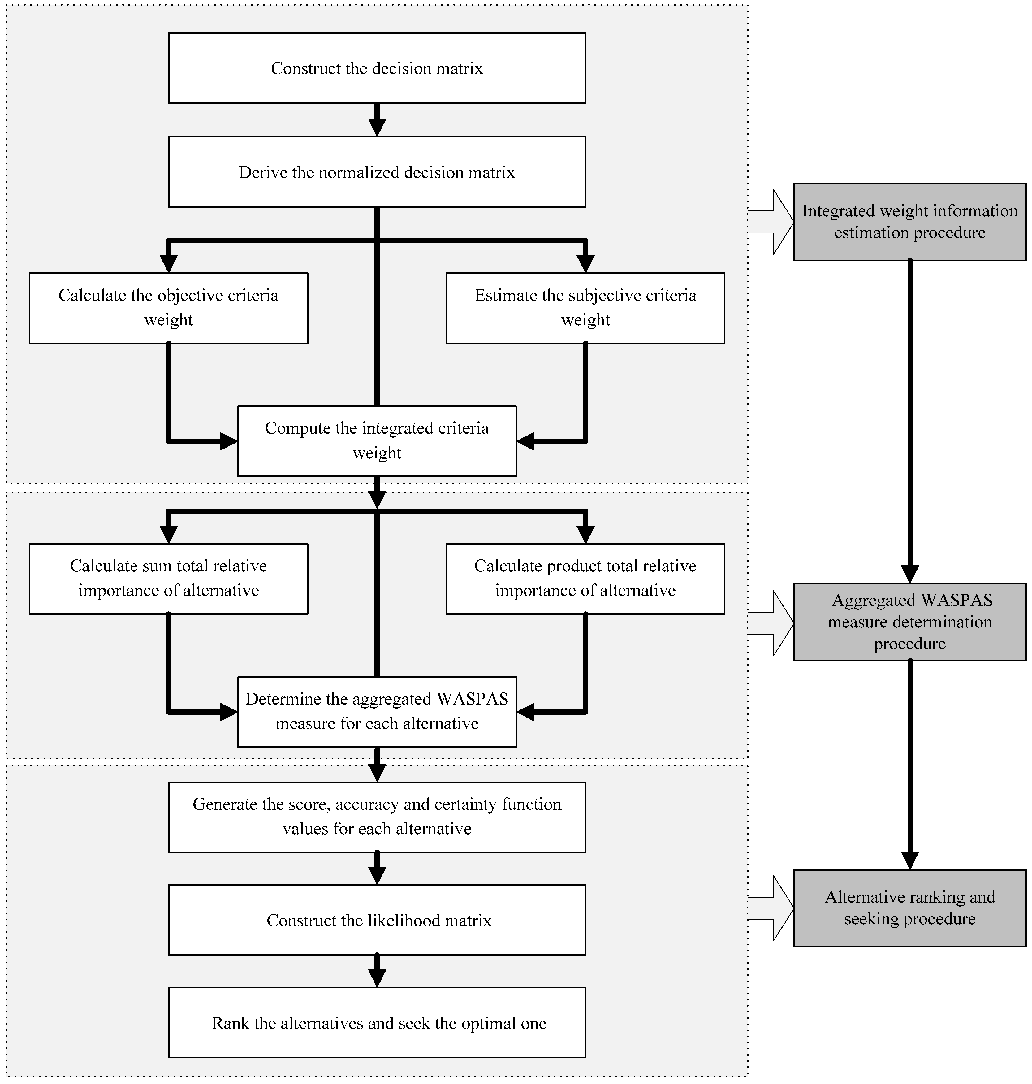
3.3. An Extended WASPAS Technique with Integrated Criteria Weight Information

The WASPAS method [34] is a well-known decision-making technique which can effectively increase the ranking accuracy by integrating WSM and WPM. It has better accuracy than only using one of WSM or WPM, which has been proved in [34]. Total importance of an alternative is determined by the aggregated WASPAS measure, which is in essence a joint criterion derived from the use of weighted arithmetic and geometric averaging operators simultaneously [66]. The feasible ranking order can be ensured by altering the parameter between the sum total relative importance and the product total relative importance of alternative computed by theses operators within the completely unknown criteria information.

In most practical cases, the criteria weight information tends to be completely unknown, and there commonly exists relationship among alternatives. To this end, this paper combines the objective weight and subjective weight acquisition methods defined above to reflect more realistic weight information in the integrated weight information estimation procedure of the newly extended WASPAS technique. It is well known that a PA operator can effectively reveal the relationship among alternatives by calculating support degrees from others [67]. The PA operator is generalized into the WASPAS method to optimize the aggregated WASPAS measure determination procedure in this paper. Consider the human beings’ expression preference and the uncertainty they faced with, this paper proposes an extended WASPAS technique in which three procedures are feasibly implemented under INSs context. The framework of the extended technique is displayed in Figure 1.

Assume that a MCDM problem in which a permutation of $m$ alternatives $\left\{A_1,\cdots ,A_i,\cdots ,A_m\right\}$ are evaluated under a permutation of $n$ criteria $\left\{C_1,\cdots ,C_j,\cdots ,C_n\right\}$. The performance evaluation of the $i$ th alternative on the $j$ th criteria is assessed by the INSs denoted by $a_{ij}=\langle \left[T_{ij}^L,T_{ij}^U\right],\left[I_{ij}^L,I_{ij}^U\right],\left[F_{ij}^L,F_{ij}^U\right]\rangle$. The main procedures are outlined as follows:

Step 1.

Construct the decision matrix.

Let a DM provide performance estimation of every alternative with respect to all the criteria, which is shown as

$$A={\left(A_{ij}\right)}_{m\times n}={\left[\begin{array}{cccc}{a}_{11}& a_{12}& \dots & a_{1n}\\ a_{21}& a_{22}& \dots & a_{2n}\\ & & ⋮& \\ a_{n1}& a_{n2}& \dots & a_{nn}\end{array}\right]}_{m\times n}$$

Step 2.

Derive the normalized decision matrix.

Utilize Equation (1) in Definition 4 to convert the evaluation under cost criteria to benefit criteria. For convenience, the normalized evaluations for the $i$th alternative with respect to the $j$th cost criteria are also denoted by $a_{ij}=\langle \left[T_{ij}^L,T_{ij}^U\right],\left[I_{ij}^L,I_{ij}^U\right],\left[F_{ij}^L,F_{ij}^U\right]\rangle$.

Step 3.

Calculate the objective criteria weight.

Use Equations (16) and (17) to calculate the objective weight ${\omega }_j^{\prime *}$ for each criteria by the maximizing deviation method.

Step 4.

Estimate the subjective criteria weight.

Conduct the procedures proposed in Section 3.2, and estimate the subjective criteria weight ${\omega }_j^{″}$ for each criteria.

Step 5.

Compute the integrated criteria weight.

Combine the objective and subjective weights generated from Step 3 and Step 4, the integrated criteria weight ${\omega }_j$ is shown as

$${\omega }_j=\lambda {\omega }_j^{\prime *}+\left(1-\lambda \right){\omega }_j^{″},$$

(20)

in which $\lambda$ is the aggregation parameter altering in $\left[0,1\right]$.

Step 6.

Calculate sum total relative importance of alternative.

Incorporate the INPWA operator defined in Equation (9), the sum total relative importance of alternative $i$ is calculated by Equation (21).

$$Q_i^{\prime }=INPWA\left(a_1,a_2,\cdots ,a_n\right).$$

(21)

Step 7.

Calculate product total relative importance of alternative.

Refer to the INPGWA operator in Equation (8), the product total relative importance for alternative $i$ is defined as

$$Q_i^{″}=INPGWA\left(a_1,a_2,\cdots ,a_n\right).$$

(22)

Step 8.

Determine the aggregated WASPAS measure for each alternative.

Aggregate $Q_i^{\prime }$ and $Q^{″}$, the final WASPAS measure can be determined by the equation as follows:

$$Q_j=\theta Q_i^{\prime }+\left(1-\theta \right)Q_i^{″},$$

(23)

in which $\theta$ is the parameter to adjust the proportion of WSM and WPM in the WASPAS technique altering in $\left[0,1\right]$. When $\theta =1$, the WASPAS technique is degenerated to WSM. When $\theta =0$, the WASPAS technique is degenerated to WPM.

Step 9.

Generate the score, accuracy and certainty function values for each alternative.

Obtain the score, accuracy and certainty function values $S\left(a_i\right)$, $H\left(a_i\right)$ and $B\left(a_i\right)$ for each alternative utilizing Equation (1) in Definition 7.

Step 10.

Construct the likelihood matrix.

Construct the possibility matrix of the score function value $S\left(a_i\right)$ according to Equation (2), which is shown as follows:

$$P^S\left(S\left(a_i\right)\ge S\left(a_j\right)\right)={\left[\begin{array}{cccc}{p}_{11}^S& p_{12}^S& \cdots & p_{1n}^S\\ p_{21}^S& p_{22}^S& \cdots & p_{2n}^S\\ & & ⋮& \\ p_{n1}^S& p_{n2}^S& \cdots & p_{nn}^S\end{array}\right]}_{n\times n},$$

whose elements $p_{ij}^S$ represents the possibility degree of $S\left(a_i\right)\ge S\left(a_j\right)$. If $p_{ij}^S=0.5$, then calculate the possibility degree of $H\left(a_i\right)\ge H\left(a_j\right)$ characterized by $p_{ij}^H$. If $p_{ij}^H=0.5$, then calculate the possibility degree of $B\left(a_i\right)\ge B\left(a_j\right)$ characterized by $p_{ij}^B$. Obtain the ranking vector $p_i$ according to Equation (4).

Step 11.

Rank the alternatives and select the good location.

Rank all the alternatives and select the good location according to the descending order of $p_i(i=1,2,\cdots ,m)$.

4. Case Study

4.1. Problem Description

With the increasing concern of the regional competition and circumstance protection, solar-wind power station contributes to converting solar or wind resources into power, and further generating electric energy. When assuming that government planners want to build a solar-wind power station for better serving regional socio-economy, a good station construction location should be selected. A group of experts are invited to consist a working team for evaluating four locations $A_i$$\left(i=1,2,\cdots ,4\right)$ with respect to various influential factors utilizing numerical rating in the range from 0 to 1. According to relative literature research, this paper concludes its influential factors into five criteria in

Table 2. Criteria information and relative description.

Criteria ${\mathit{C}}_{\mathit{j}}$	Description
Natural resources $C_1$	Natural resources include various indicators related to wind and solar resources in the location.
Economic factors $C_2$	Economic factors briefly measure the cost during the engineering construction, operation and maintenance procedures.
Traffic conditions $C_3$	Traffic conditions reflect the traffic convenience to the location during the engineering construction, operation and maintenance procedures.
Environmental factors $C_4$	Environmental factors reflect the environment destruction during the engineering construction and operation procedures.
Social factors $C_5$	Social factors reflect the attitude of the local residents to the engineering.

. In practical assessment procedure, the evaluation rating not only contains the numerical rating but also the emotional tendency of DMs. For a candidate location $i$ under certain criteria $j$, the positive maximum evaluation among all the DMs is treated as the $T_{ij}^U$ in the INS $a_{ij}=\langle \left[T_{ij}^L,T_{ij}^U\right],\left[I_{ij}^L,I_{ij}^U\right],\left[F_{ij}^L,F_{ij}^U\right]\rangle$, and the negative minimum evaluation of the entire working team is treated as $F_{ij}^L$ in the INS. For instance, when rating for location $A_1$ with respect to economic factors $C_2$, the maximum and minimum evaluation from all the experts, who deem it is appropriate to construct the station here, are 0.5, 0.3, respectively; the maximum and minimum of inappropriate evaluation are 0.8, 0.2; the maximum and minimum of the other experts are 0.3, 0.2; then, the INS can be expressed as $a_{12}=\langle \left[0.3,0.5\right],\left[0.2,0.8\right],\left[0.2,0.3\right]\rangle$. Based on this principle, final decision matrix $A={\left(A_{ij}\right)}_{m\times n}$ involving the synthetic evaluation information from all the DMs in the working group is derived as follows:

$$\begin{array}{l}A={\left(A_{ij}\right)}_{4\times 5}=[\begin{array}{cc}\langle \left[0.7,0.8\right],\left[0.5,0.7\right],\left[0.1,0.2\right]\rangle & \langle \left[0.3,0.5\right],\left[0.2,0.8\right],\left[0.2,0.3\right]\rangle \\ \langle \left[0.6,0.8\right],\left[0.4,0.5\right],\left[0.3,0.3\right]\rangle & \langle \left[0.5,0.7\right],\left[0.3,0.5\right],\left[0.1,0.3\right]\rangle \\ \langle \left[0.8,0.8\right],\left[0.4,0.6\right],\left[0.1,0.2\right]\rangle & \langle \left[0.6,0.6\right],\left[0.2,0.3\right],\left[0.4,0.5\right]\rangle \\ \langle \left[0.7,0.9\right],\left[0.3,0.4\right],\left[0.2,0.2\right]\rangle & \langle \left[0.6,0.8\right],\left[0.4,0.4\right],\left[0.2,0.4\right]\rangle \end{array}\\ {\begin{array}{ccc}\langle \left[0.4,0.6\right],\left[0.2,0.2\right],\left[0.2,0.4\right]\rangle & \langle \left[0.4,0.5\right],\left[0.5,0.6\right],\left[0.4,0.4\right]\rangle & \langle \left[0.6,0.7\right],\left[0.4,0.5\right],\left[0.4,0.5\right]\rangle \\ \langle \left[0.6,0.7\right],\left[0.4,0.6\right],\left[0.3,0.4\right]\rangle & \langle \left[0.5,0.6\right],\left[0.3,0.4\right],\left[0.4,0.5\right]\rangle & \langle \left[0.8,0.9\right],\left[0.3,0.4\right],\left[0.1,0.2\right]\rangle \\ \langle \left[0.7,0.8\right],\left[0.6,0.7\right],\left[0.1,0.2\right]\rangle & \langle \left[0.6,0.7\right],\left[0.7,0.8\right],\left[0.2,0.3\right]\rangle & \langle \left[0.7,0.8\right],\left[0.5,0.6\right],\left[0.1,0.2\right]\rangle \\ \langle \left[0.5,0.6\right],\left[0.5,0.6\right],\left[0.2,0.3\right]\rangle & \langle \left[0.8,0.9\right],\left[0.3,0.4\right],\left[0.1,0.2\right]\rangle & \langle \left[0.5,0.7\right],\left[0.5,0.6\right],\left[0.2,0.3\right]\rangle \end{array}]}_{4\times 5}\end{array}$$

4.2. The Selection of Solar-Wind Power Station Location

The specific procedures of seeking a good solar-wind power station location with the extended WASPAS technique are implemented as follows:

Step 1.

Construct the decision matrix.

The decision matrix is constructed by the illustration in Section 4.1, which is shown as $A={\left(A_{ij}\right)}_{4\times 5}$ above.

Step 2.

Derive the normalized decision matrix.

Referring to the criteria description in Table 2, $C_2$ and $C_4$ are cost criteria. Utilize Equation (1) in Definition 4, the normalized decision matrix can be obtained as

$$\begin{array}{l}A={\left(A_{ij}\right)}_{4\times 5}=[\begin{array}{cc}\langle \left[0.7,0.8\right],\left[0.5,0.7\right],\left[0.1,0.2\right]\rangle & \langle \left[0.2,0.3\right],\left[0.2,0.8\right],\left[0.3,0.5\right]\rangle \\ \langle \left[0.6,0.8\right],\left[0.4,0.5\right],\left[0.3,0.3\right]\rangle & \langle \left[0.1,0.3\right],\left[0.5,0.7\right],\left[0.5,0.7\right]\rangle \\ \langle \left[0.8,0.8\right],\left[0.4,0.6\right],\left[0.1,0.2\right]\rangle & \langle \left[0.4,0.5\right],\left[0.7,0.8\right],\left[0.6,0.6\right]\rangle \\ \langle \left[0.7,0.9\right],\left[0.3,0.4\right],\left[0.2,0.2\right]\rangle & \langle \left[0.2,0.4\right],\left[0.6,0.6\right],\left[0.6,0.8\right]\rangle \end{array}\\ {\begin{array}{ccc}\langle \left[0.4,0.6\right],\left[0.2,0.2\right],\left[0.2,0.4\right]\rangle & \langle \left[0.4,0.4\right],\left[0.4,0.5\right],\left[0.4,0.5\right]\rangle & \langle \left[0.6,0.7\right],\left[0.4,0.5\right],\left[0.4,0.5\right]\rangle \\ \langle \left[0.6,0.7\right],\left[0.4,0.6\right],\left[0.3,0.4\right]\rangle & \langle \left[0.4,0.5\right],\left[0.6,0.7\right],\left[0.5,0.6\right]\rangle & \langle \left[0.8,0.9\right],\left[0.3,0.4\right],\left[0.1,0.2\right]\rangle \\ \langle \left[0.7,0.8\right],\left[0.6,0.7\right],\left[0.1,0.2\right]\rangle & \langle \left[0.2,0.3\right],\left[0.2,0.3\right],\left[0.6,0.7\right]\rangle & \langle \left[0.7,0.8\right],\left[0.5,0.6\right],\left[0.1,0.2\right]\rangle \\ \langle \left[0.5,0.6\right],\left[0.5,0.6\right],\left[0.2,0.3\right]\rangle & \langle \left[0.1,0.2\right],\left[0.6,0.7\right],\left[0.8,0.9\right]\rangle & \langle \left[0.5,0.7\right],\left[0.5,0.6\right],\left[0.2,0.3\right]\rangle \end{array}]}_{4\times 5}\end{array}$$

Step 3.

Calculate the objective criteria weight.

Use Equations (16) and (17), then the objective weight ${\omega }_j^{\prime *}$ for each criteria can be calculated as

$${\omega }_1^{\prime *}=0.1259,{\omega }_2^{\prime *}=0.2122,{\omega }_3^{\prime *}=0.2086,{\omega }_4^{\prime *}=0.2698,{\omega }_5^{\prime *}=0.1835.$$

Step 4.

Estimate the subjective criteria weight.

Assume that the aggregation parameter $\lambda =0.5$, and the order relation of all the criteria is $C_4\succ C_2\succ C_1\succ C_5\succ C_3$ judging from DMs’ subjective experience. Referring to the relative importance degree index among adjacent criteria in Table 1, the subjective criteria weight for each criteria is estimated as ${\omega }_1^{″}=0.3533$, ${\omega }_2^{″}=0.2945$, ${\omega }_3^{″}=0.1840$, ${\omega }_4^{″}=0.1022$ and ${\omega }_5^{″}=0.0639$.

Step 5.

Compute the integrated criteria weight.

Combine the objective and subjective weights generated from Step 3 and Step 4, the integrated weight of criteria is shown as ${\omega }_1=0.2396$, ${\omega }_2=0.2534$, ${\omega }_3=0.1963$, ${\omega }_4=0.1860$ and ${\omega }_5=0.1237$.

Step 6.

Calculate sum total relative importance of alternative.

Incorporate the INPWA operator defined in Equation (9), the sum total relative importance of all alternatives are

$$Q_1^{\prime }=\langle \left[0.4986,0.6171\right],\left[0.3084,0.6468\right],\left[0.1866,0.3342\right]\rangle ,$$

$$Q_2^{\prime }=\langle \left[0.4236,0.6255\right],\left[0.4479,0.5977\right],\left[0.3746,0.4618\right]\rangle ,$$

$$Q_3^{\prime }=\langle \left[0.6136,0.6642\right],\left[0.5212,0.6680\right],\left[0.2643,0.3665\right]\rangle$$

$$Q_4^{\prime }=\langle \left[0.4867,0.7214\right],\left[0.4433,0.5128\right],\left[0.3468,0.4122\right]\rangle$$

Step 7.

Calculate product total relative importance of alternative.

Refer to the INPGWA operator in Equation (8), the product total relative importance for alternatives are

$$Q_1^{″}=\langle \left[0.3816,0.4983\right],\left[0.3562,0.7138\right],\left[0.2219,0.3815\right]\rangle ,$$

$$Q_2^{″}=\langle \left[0.2638,0.4970\right],\left[0.4566,0.6189\right],\left[0.4046,0.5409\right]\rangle ,$$

$$Q_3^{″}=\langle \left[0.5184,0.6005\right],\left[0.5784,0.7099\right],\left[0.4203,0.4605\right]\rangle$$

$$Q_4^{″}=\langle \left[0.3533,0.5616\right],\left[0.4852,0.5355\right],\left[0.4509,0.6134\right]\rangle$$

Step 8.

Determine the aggregated WASPAS measure for each alternative.

Let $\theta =0.5$, then the final WASPAS measure can be derived as

$$Q_1=\langle \left[0.4401,0.5577\right],\left[0.3323,0.6803\right],\left[0.2043,0.3579\right]\rangle ,$$

$$Q_2=\langle \left[0.3437,0.5613\right],\left[0.4523,0.6083\right],\left[0.3896,0.5014\right]\rangle ,$$

$$Q_3=\langle \left[0.5660,0.6324\right],\left[0.5498,0.6889\right],\left[0.3423,0.4135\right]\rangle$$

$$Q_4=\langle \left[0.4200,0.6415\right],\left[0.4643,0.5241\right],\left[0.3989,0.5129\right]\rangle$$

Step 9.

Generate the score, accuracy and certainty function values for each alternative.

For each alternative, the score, accuracy and certainty function values $S\left(a_i\right)$, $H\left(a_i\right)$ and $B\left(a_i\right)$ are shown in

Table 3. Relative function values of alternatives.

${\mathit{A}}_{\mathit{i}}$	$\mathit{S}\left({\mathit{a}}_{\mathit{i}}\right)$	$\mathit{H}\left({\mathit{a}}_{\mathit{i}}\right)$	$\mathit{B}\left({\mathit{a}}_{\mathit{i}}\right)$
$A_1$	$\left[1.4020,2.0212\right]$	$\left[0.1998,0.2359\right]$	$\left[0.4401,0.5577\right]$
$A_2$	$\left[1.2341,1.7194\right]$	$\left[-0.0459,0.0599\right]$	$\left[0.3437,0.5613\right]$
$A_3$	$\left[1.4636,1.7402\right]$	$\left[0.2189,0.2237\right]$	$\left[0.5660,0.6324\right]$
$A_4$	$\left[1.3831,1.7783\right]$	$\left[0.0212,0.1286\right]$	$\left[0.4200,0.6415\right]$

.

Step 10.

Construct the likelihood matrix.

Construct the possibility matrix of the score function value $S\left(a_i\right)$ according to Equation (2), which is shown as follows:

$$P^S\left(S\left(a_i\right)\ge S\left(a_j\right)\right)={\left[\begin{array}{cccc}0.5& 0.7126& 0.6224& 0.6290\\ 0.7126& 0.5& 0.3358& 0.3820\\ 0.6224& 0.3358& 0.5& 0.5315\\ 0.6290& 0.3820& 0.5315& 0.5\end{array}\right]}_{4\times 4}.$$

And the ranking vector can be obtained as $p_1=2.5981$, $p_2=2.1977$, $p_3=2.2423$ and $p_4=2.2819$.

Step 11.

Rank the alternatives and select the good location.

The ranking order of all the alternatives is $A_1\succ A_4\succ A_3\succ A_2$ and the good location is $A_1$.

5. Sensitivity Analysis and Comparison Analysis

In this section, comparison analysis and sensitivity analysis are conducted to further testify the effectiveness and reliability of the extended WASPAS technique with existing methods on the same example.

5.1. Sensitivity Analysis and Discussion

To demonstrate the impact of different aggregation parameter $\lambda$ and the proportion adjustment parameter $\theta$ on the final location selection results, we conduct the sensitivity analysis on the same example with five $\lambda$$\left(0,0.2,0.5,0.8,1\right)$ values and five $\theta$$\left(0,0.2,0.5,0.8,1\right)$ values simultaneously. The ranking results for different $\lambda$ and $\theta$ are displayed in

Table 4. Ranking results for different $\lambda$ and $\theta$.

$\mathit{\lambda }$	$\mathit{\theta }=0$	$\mathit{\theta }=0.2$	$\mathit{\theta }=0.5$	$\mathit{\theta }=0.8$	$\mathit{\theta }=1$
$0$	$A_1\succ A_4\succ A_3\succ A_2$	$A_1\succ A_4\succ A_3\succ A_2$	$A_1\succ A_4\succ A_3\succ A_2$	$A_1\succ A_4\succ A_3\succ A_2$	$A_1\succ A_4\succ A_3\succ A_2$
$0.2$	$A_4\succ A_1\succ A_3\succ A_2$	$A_4\succ A_1\succ A_3\succ A_2$	$A_1\succ A_4\succ A_3\succ A_2$	$A_1\succ A_4\succ A_3\succ A_2$	$A_1\succ A_4\succ A_3\succ A_2$
$0.5$	$A_4\succ A_1\succ A_3\succ A_2$	$A_4\succ A_1\succ A_3\succ A_2$	$A_4\succ A_1\succ A_3\succ A_2$	$A_4\succ A_1\succ A_3\succ A_2$	$A_4\succ A_1\succ A_3\succ A_2$
$0.8$	$A_4\succ A_1\succ A_3\succ A_2$	$A_4\succ A_1\succ A_3\succ A_2$	$A_1\succ A_4\succ A_3\succ A_2$	$A_1\succ A_4\succ A_3\succ A_2$	$A_1\succ A_4\succ A_3\succ A_2$
$1$	$A_4\succ A_1\succ A_3\succ A_2$	$A_4\succ A_1\succ A_3\succ A_2$	$A_4\succ A_1\succ A_3\succ A_2$	$A_4\succ A_1\succ A_3\succ A_2$	$A_4\succ A_1\succ A_3\succ A_2$

.

The variation of $\lambda$ represents the influence of criteria weight integrated by objective and subjective weights to final selection results. In addition, altering the $\theta$ values means that the change from sum total relative importance to product total relative importance. Synthetizing what is shown in Table 4, it can be inferred that different $\lambda$ and $\theta$ values indeed affect final selection results. When $\lambda =0$ and $\lambda =1$, the integrated criteria weight is complete subjective or objective weight, and the ranking order has different selection results $A_1$ and $A_4$ under these opposite context. Furthermore, no matter how the variation of $\theta$ values, the ranking order remains all the same in these circumstances. When $\lambda =0.2$ and $\lambda =0.8$, the proportion adjustment parameter $\theta$ values make huge differences to the ranking order. The ranking result yields $A_4\succ A_1\succ A_3\succ A_2$ when $0\le \theta <0.5$, while it yields $A_1\succ A_4\succ A_3\succ A_2$ when $0.5\le \theta \le 1$. In view of the identical changeable tendency of ranking order, it is apparent that the gradual increase of the adjustment proportion $\theta$ clearly affects the order when different importance of the objective and subjective weights in the integrated weight. However, when the importance of the objective and subjective weights in the integrated weight are totally equivalent, the ranking order keeps $A_4\succ A_1\succ A_3\succ A_2$ all the time.

Obviously, these ranking order and selection results reveal that different $\lambda$ and $\theta$ values have an effect on the decision-making procedure. It further indicates that the combination of objective and subjective weights, and the integration of sum total relative importance and product total relative importance emphasize the influence to the selection procedure. Integrated the specific meaning of $\lambda$ and $\theta$ with their role playing in the decision-making procedures, the location selection becomes a dynamic procedure by setting different parameter values derived from practical context.

5.2. Comparison Analysis and Discussion

This subsection further validates the effectiveness and reliability of the newly proposed method by comparing it with different existing methods on the identical illustrative example. The ranking results are shown in

Table 5. Ranking results with different existing methods.

Methods	Ranking Results
Similarity measure in [62]	$A_4\succ A_2\succ A_3\succ A_1$
An extended TOPSIS method in [69]	$A_3\succ A_4\succ A_2\succ A_1$
Method used weighted arithmetic aggregation operator in [68]	$A_4\succ A_1\succ A_3\succ A_2$
Method used weighted geometric aggregation operator in [68]	$A_4\succ A_1\succ A_3\succ A_2$
Classical WASPAS method in [34]	$A_4\succ A_1\succ A_3\succ A_2$
The proposed method	$A_1\succ A_4\succ A_3\succ A_2$

. As there exists no relative criteria weight obtainment method in [34,62,68] chosen for comparison, we use the integrated criteria weight obtained in this paper as the criteria weight information for the comparison convenience.

(1)

The method in [62] generates the selection result by implementing two steps. Firstly, confirm the ideal alternatives for different type of criteria. Subsequently, derive the result by similarity measures. According to the first similarity measure in that literature, the similarity measures are obtained as $S_1^{*}\left(A^{*},A_1\right)=0.8178$, $S_1^{*}\left(A^{*},A_2\right)=0.8705$, $S_1^{*}\left(A^{*},A_3\right)=0.8692$ and $S_1^{*}\left(A^{*},A_4\right)=0.9057$.

(2)

In the method of [69], maximizing deviation method is utilized to derive objective weights. Then, based on the ideal of TOPSIS method, alternatives are ranked by the relative closeness coefficient. Conduct these procedures, relative closeness coefficient can be calculated as $RC{C}_1=0.5226$, $RC{C}_2=0.5186$, $RC{C}_3=0.5190$ and $RC{C}_4=0.5189$.

(3)

The procedure of the method in [68] can be briefly classified into aggregation process and ranking process. The ranking procedure in [68] is identical with our proposed method. Based on weighted arithmetic aggregation operator or weighted geometric aggregation operator, the total score are obtained as $p_s=\left[2.2997,2.0098,2.0589,2.5926\right]$ or $p_s=\left[2.5804,2.2751,2.3728,2.9288\right]$ with the same ranking order $A_4\succ A_1\succ A_3\succ A_2$.

(4)

Classical WASPAS method in [34] generates the final WASPAS measure by aggregating weighted arithmetic aggregation operator and weighted geometric aggregation operator. To better compare the classical WASPAS method with our method, the alternatives are ranked by the ranking procedure in our paper. Then, ranking vector can be obtained as $p_1=2.4449$, $p_2=2.1483$, $p_3=2.2189$ and $p_4=2.7681$.

It can be easily inferred from Table 5 that different methods generate totally distinct selection results. Especially, the order sequence derived from the methods in [62,69] is entirely opposite to ours. The good location selection for [62,69] and our paper are $A_4$, $A_3$ and $A_1$, respectively. The primary reason for that phenomenon relies on that these methods were proposed based on completely different ideal. It results in the inconsistent sequence between each pair of alternatives in these methods. Both the similarity measures and TOPSIS method rank the alternatives on the ideal of distance. For a better comparison analysis, we adopt Hamming distance during the calculation procedure. Moreover, the method in [62] neglects the relation of criteria to each other, while the method in [69] only considers the objective criteria weight without focusing on the subjective preference of DMs. The proposed method emphasizes the support relation from other criteria in the course of WASPAS measure determination. It adequately considers the objective criteria weights and subjective experience judgement from DMs by integrated criteria weight. The selection $A_4$ and $A_3$ cannot reflect realistic situation without considering the subjective criteria during the MCDM procedure. In addition, these characteristics ensure the effectiveness and reliability of the location selection $A_1$ derived from our method. Although both the method in [68] and our method utilize an identical ranking method, the aggregation operators cause huge differences to the final location selection. When using one of the weighted arithmetic aggregation operator or weighted geometric aggregation operator in [68], it yields identical selection result $A_4$. However, the proposed method not only contains the advantage of PA operator, but also effectively utilizes the combination of INPGWA and INPWA rather than applying them respectively. Besides, the extended WASPAS technique reveals its superiority by implementing three procedures to assure the selection result $A_1$ rational and convincing.

Utilizing identical aggregation operator, methods in [34,68] provide the totally same ranking order $A_4\succ A_1\succ A_3\succ A_2$ with identical location selection $A_4$. It indicates that the superiority of the classical WASPAS method cannot be inferred because there exists no ranking or selection discrepancy when using completely different methods. It is obvious that the ranking and selection results of the classical WASPAS method and the proposed method exists discrepancy. The order of $A_1$ and $A_4$ is opposite in those methods. That is, though both the classical and extended WASPAS methods have the same procedure in which the WASPAS measure are aggregated by two kinds of operators, the extended WASPAS method reflects a more rational selection result by newly incorporating the advantage of PA operators in that. Furthermore, the integrated weight information estimation procedure further ensures the selection of the extended WASPAS method scientific. The identical order between alternatives $A_3$ and $A_2$ in these methods can verify the effectiveness of the extended one.

From above discussion, primary highlights of the newly extended WASPAS technique can be simply summarized into the following points.

(1)

It can effectively manage the solar-wind power station location problem via embedding three procedures into the newly extended WASPAS technique. During the WASPAS technique implement process, a rational location selection result will be generated by incorporating the advantages of relevant methods in these procedures.

(2)

With the maximizing derivation method, objective criteria weights can be simply determined no matter under the criteria weights completely unknown or incomplete circumstances. Apart from the objective criteria weights, subjective weights, which fully reflect the subjective preference under practice, can be obtained with G1. The integrated criteria weight is the combination of the objective and subjective weights, and can adequately represent more realistic situation.

(3)

Different aggregation parameter $\lambda$ and the proportion adjustment parameter $\theta$ facilitate the whole procedures a dynamic selection. The parameter setting is based on the requirement of real application and subjective preference of DMs, which makes the extended WASPAS technique feasible in dealing with the reality.

6. Conclusions

A good location of the solar-wind power station can affect regional competitiveness and direct future development to a great extent. Faced with multiple uncertainties in reality, the location selection case is considered within the INSs circumstances for tackling such challenges. Recognized as a complex MCDM procedure, the selection in this paper is settled by an extended WASPAS technique containing three procedures to reinforce its applicability to real situation. For modelling more realistic information, some modifications are made in the classical WASPAS method especially utilizing the objective and subjective criteria weight integrated weight information. Its strengths have been adequately discussed via comparison analysis and sensitivity analysis.

Highlights of the extended technique can be briefly summarized in three aspects. Firstly, it ensures a relatively rational and scientific result by incorporating three procedures into the framework of the technique. Secondly, the integrated weight information reflects more realistic weight information with the combination of the objective and subjective criteria weight information. Thirdly, more practical contexts can be reflected by altering the aggregation parameter and the proportion adjustment parameter during performing relevant procedures. Although the location selection case can be well measured by the criteria dimensions in this paper, potential work should also be focused on specific sub-criteria information for reaching a more promising solution.

References

1. Khare, V.; Nema, S.; Baredar, P. Status of solar wind renewable energy in India. Renew. Sustain. Energy Rev. 2013, 27, 1–10. [Google Scholar] [CrossRef]
2. Khare, V.; Nema, S.; Baredar, P. Solar–wind hybrid renewable energy system: A review. Renew. Sustain. Energy Rev. 2016, 58, 23–33. [Google Scholar] [CrossRef]
3. Kazem, H.A.; Al-Badi, H.A.S.; Al Busaidi, A.S.; Chaichan, M.T. Optimum design and evaluation of hybrid solar/wind/diesel power system for Masirah Island. Environ. Dev. Sustain. 2016, 1–18. [Google Scholar] [CrossRef]
4. Petrakopoulou, F.; Robinson, A.; Loizidou, M. Simulation and evaluation of a hybrid concentrating-solar and wind power plant for energy autonomy on islands. Renew. Energy 2016, 96, 863–871. [Google Scholar] [CrossRef]
5. Jahangiri, M.; Ghaderi, R.; Haghani, A.; Nematollahi, O. Finding the best locations for establishment of solar-wind power stations in Middle-East using GIS: A review. Renew. Sustain. Energy Rev. 2016, 66, 38–52. [Google Scholar] [CrossRef]
6. Lee, A.H.I.; Kang, H.Y.; Liou, Y.J. A hybrid multiple-criteria decision-making approach for photovoltaic solar plant location selection. Sustainability 2017, 9, 184. [Google Scholar] [CrossRef]
7. Roy, B. Multicriteria Methodology for Decision Aiding; Springer Science & Business Media: Dordrecht, The Netherlands, 2013. [Google Scholar]
8. Roy, B. Paradigms and challenges. In Multiple Criteria Decision Analysis: STATE of the Art Surveys; Figueira, J., Greco, S., Ehrgott, M., Eds.; Springer: New York, NY, USA, 2005; Volume 78, pp. 3–24. [Google Scholar]
9. Roy, B.; Słowiński, R. Questions guiding the choice of a multicriteria decision aiding method. EURO J. Decis. Process. 2013, 1, 69–97. [Google Scholar] [CrossRef]
10. Abudeif, A.M.; Abdel Moneim, A.A.; Farrag, A.F. Multicriteria decision analysis based on analytic hierarchy process in GIS environment for siting nuclear power plant in Egypt. Ann. Nucl. Energy 2015, 75, 682–692. [Google Scholar] [CrossRef]
11. Latinopoulos, D.; Kechagia, K. A GIS-based multi-criteria evaluation for wind farm site selection. A regional scale application in Greece. Renew. Energy 2015, 78, 550–560. [Google Scholar] [CrossRef]
12. Liu, J.; Xu, F.; Lin, S. Site selection of photovoltaic power plants in a value chain based on grey cumulative prospect theory for sustainability: A case study in Northwest China. J. Clean. Prod. 2017, 148, 386–397. [Google Scholar] [CrossRef]
13. Wu, Y.; Chen, K.; Zeng, B.; Yang, M.; Li, L.; Zhang, H. A cloud decision framework in pure 2-tuple linguistic setting and its application for low-speed wind farm site selection. J. Clean. Prod. 2017, 142, 2154–2165. [Google Scholar] [CrossRef]
14. Wu, Y.; Zhang, J.; Yuan, J.; Geng, S.; Zhang, H. Study of decision framework of offshore wind power station site selection based on ELECTRE-III under intuitionistic fuzzy environment: A case of China. Energy Convers. Manag. 2016, 113, 66–81. [Google Scholar] [CrossRef]
15. Jun, D.; Tian-tian, F.; Yi-sheng, Y.; Yu, M. Macro-site selection of wind/solar hybrid power station based on ELECTRE-II. Renew. Sustain. Energy Rev. 2014, 35, 194–204. [Google Scholar] [CrossRef]
16. Yunna, W.; Geng, S. Multi-criteria decision making on selection of solar-wind hybrid power station location: A case of China. Energy Convers. Manag. 2014, 81, 527–533. [Google Scholar] [CrossRef]
17. Zhang, H.Y.; Peng, H.G.; Wang, J.; Wang, J.Q. An extended outranking approach for multi-criteria decision-making problems with linguistic intuitionistic fuzzy numbers. Appl. Soft Comput. 2017, 59, 462–474. [Google Scholar] [CrossRef]
18. Turksen, I.B. Interval valued fuzzy sets based on normal forms. Fuzzy Sets Syst. 1986, 20, 191–210. [Google Scholar] [CrossRef]
19. Nie, R.; Wang, J.; Li, L. 2-tuple linguistic intuitionistic preference relation and its application in sustainable location planning voting system. J. Intell. Fuzzy Syst. 2017. [Google Scholar] [CrossRef]
20. Cao, Y.X.; Zhou, H.; Wang, J.Q. An approach to interval-valued intuitionistic stochastic multi-criteria decision-making using set pair analysis. Int. J. Mach. Learn. Cybern. 2016, 1–12. [Google Scholar] [CrossRef]
21. Tian, Z.P.; Wang, J.; Wang, J.Q.; Zhang, H.Y. An improved MULTIMOORA approach for multi-criteria decision-making based on interdependent inputs of simplified neutrosophic linguistic information. Neural Comput. Appl. 2016. [Google Scholar] [CrossRef]
22. Smarandache, F. Neutrosophy: Neutrosophic Probability, Set, and Logic; American Research Press: Rehoboth, DE, USA, 1998; pp. 1–105. [Google Scholar]
23. Peng, H.; Zhang, H.; Wang, J. Probability multi-valued neutrosophic sets and its application in multi-criteria group decision-making problems. Neural Comput. Appl. 2016, 1–21. [Google Scholar] [CrossRef]
24. Tian, Z.P.; Wang, J.; Wang, J.Q.; Zhang, H.Y. Simplified neutrosophic linguistic multi-criteria group decision-making approach to green product development. Group Decis. Negot. 2017, 26, 597–627. [Google Scholar] [CrossRef]
25. Smarandache, F. A Unifying Field in Logics: Neutrosophic Logic. Mult. Log. 1999, 8, 489–503. [Google Scholar]
26. Liu, C. Interval neutrosophic fuzzy stochastic multi-criteria decision-making methods based on MYCIN certainty factor and prospect theory. Rev. Tec. Fac. Ing. Univ. Del Zulia 2017, 39, 52–58. [Google Scholar]
27. Ma, H.; Hu, Z.G.; Li, K.Q.; Zhang, H.Y. Toward trustworthy cloud service selection: A time-aware approach using interval neutrosophic set. Parallel Distrib. Comput. 2016, 96, 75–94. [Google Scholar] [CrossRef]
28. Reddy, R.; Reddy, D.; Krishnaiah, G. Lean supplier selection based on hybrid MCGDM approach using interval valued neutrosophic sets: A case study. Int. J. Innov. Res. Dev. 2016, 5, 291–296. [Google Scholar]
29. Ma, Y.X.; Wang, J.Q.; Wang, J.; Wu, X.H. An interval neutrosophic linguistic multi-criteria group decision-making method and its application in selecting medical treatment options. Neural Comput. Appl. 2016, 1–21. [Google Scholar] [CrossRef]
30. Tian, Z.P.; Zhang, H.Y.; Wang, J.; Wang, J.Q.; Chen, X.H. Multi-criteria decision-making method based on a cross-entropy with interval neutrosophic sets. Int. J. Syst. Sci. 2016, 47, 3598–3608. [Google Scholar] [CrossRef]
31. Peng, J.J.; Wang, J.Q.; Yang, L.J.; Qian, J. A novel multi-criteria group decision-making approach using simplified neutrosophic information. Int. J. Uncertain. Quantif. 2017. [Google Scholar] [CrossRef]
32. Wu, X.H.; Wang, J.Q. Cross-entropy measures of multi-valued neutrosophic sets and its application in selecting middle-level manager. Int. J. Uncertain. Quantif. 2017, 2, 155–172. [Google Scholar] [CrossRef]
33. Tian, Z.P.; Wang, J.; Zhang, H.Y.; Wang, J.Q. Multi-criteria decision-making based on generalized prioritized aggregation operators under simplified neutrosophic uncertain linguistic environment. Int. J. Mach. Learn. Cybern. 2016, 1–17. [Google Scholar] [CrossRef]
34. Zavadskas, E.K.; Turskis, Z.; Antucheviciene, J.; Zakarevicius, A. Optimization of weighted aggregated sum product assessment. Electron. Electr. Eng. 2012, 122, 1–3. [Google Scholar] [CrossRef]
35. Zavadskas, E.K.; Kalibatas, D.; Kalibatiene, D. A multi-attribute assessment using WASPAS for choosing an optimal indoor environment. Arch. Civ. Mech. Eng. 2016, 16, 76–85. [Google Scholar] [CrossRef]
36. Zavadskas, E.K.; Baušys, R.; Stanujkic, D.; Magdalinovic-Kalinovic, M. Selection of lead-zinc flotation circuit design by applying WASPAS method with single-valued neutrosophic set. Acta Montan. Slovaca 2017, 21, 85–92. [Google Scholar]
37. Bagočius, V.; Zavadskas, E.K.; Turskis, Z. Multi-person selection of the best wind turbine based on the multi-criteria integrated additive-multiplicative utility function. J. Civ. Eng. Manag. 2014, 20, 590–599. [Google Scholar] [CrossRef]
38. Zavadskas, E.K.; Baušys, R.; Lazauskas, M. Sustainable assessment of alternative sites for the construction of a waste incineration plant by applying WASPAS method with single-valued neutrosophic set. Sustainability 2015, 7, 15923–15936. [Google Scholar] [CrossRef]
39. Baušys, R.; Juodagalvienė, B. Garage location selection for residential house by WASPAS-SVNS method. J. Civ. Eng. Manag. 2017, 23, 421–429. [Google Scholar] [CrossRef]
40. Zavadskas, E.K.; Antucheviciene, J.; Saparauskas, J.; Turskis, Z. MCDM methods WASPAS and MULTIMOORA: Verification of robustness of methods when assessing alternative solutions. Econ. Comput. Econ. Cybern. Stud. Res. 2013, 47, 5–20. [Google Scholar]
41. Džiugaitėtumėnienė, R.; Lapinskienė, V. The multicriteria assessment model for an energy supply system of a low energy house. Eng. Struct. Technol. 2014, 6, 33–41. [Google Scholar] [CrossRef]
42. Vafaeipour, M.; Zolfani, S.H.; Derakhti, A.; Eshkalag, M.K. Assessment of regions priority for implementation of solar projects in Iran: New application of a hybrid multi-criteria decision making approach. Energy Convers. Manag. 2014, 86, 653–663. [Google Scholar] [CrossRef]
43. Ghorabaee, M.K.; Amiri, M.; Zavadskas, E.K.; Antuchevičienė, J. Assessment of third-party logistics providers using a CRITIC–WASPAS approach with interval type-2 fuzzy sets. Transport 2017, 32, 66–78. [Google Scholar] [CrossRef]
44. Zavadskas, E.K.; Turskis, Z.; Antucheviciene, J. Selecting a contractor by using a novel method for multiple attribute analysis: Weighted aggregated sum product assessment with grey values (WASPAS­G). Stud. Inform. Control. 2015, 24, 141–150. [Google Scholar] [CrossRef]
45. Mardani, A.; Nilashi, M.; Zakuan, N.; Loganathan, N.; Soheilirad, S.; Saman, M.Z.M.; Ibrahim, O. A systematic review and meta-Analysis of SWARA and WASPAS methods: Theory and applications with recent fuzzy developments. Appl. Soft Comput. 2017, 57, 265–292. [Google Scholar] [CrossRef]
46. Zavadskas, E.K.; Antucheviciene, J.; Razavi Hajiagha, S.H.; Hashemi, S.S. Extension of weighted aggregated sum product assessment with interval-valued intuitionistic fuzzy numbers (WASPAS-IVIF). Appl. Soft Comput. 2014, 24, 1013–1021. [Google Scholar] [CrossRef]
47. Wei, G.W. Maximizing deviation method for multiple attribute decision making in intuitionistic fuzzy setting. Knowl. Based Syst. 2008, 21, 833–836. [Google Scholar] [CrossRef]
48. Şahin, R.; Liu, P. Maximizing deviation method for neutrosophic multiple attribute decision making with incomplete weight information. Neural Comput. Appl. 2016, 27, 2017–2029. [Google Scholar] [CrossRef]
49. Gitinavard, H.; Mousavi, S.M.; Vahdani, B. A new multi-criteria weighting and ranking model for group decision-making analysis based on interval-valued hesitant fuzzy sets to selection problems. Neural Comput. Appl. 2016, 27, 1593–1605. [Google Scholar] [CrossRef]
50. Xu, Z.; Zhang, X. Hesitant fuzzy multi-attribute decision making based on TOPSIS with incomplete weight information. Knowl. Based Syst. 2013, 52, 53–64. [Google Scholar] [CrossRef]
51. Chen, Z.; Yang, W. A new multiple attribute group decision making method in intuitionistic fuzzy setting. Appl. Math. Model. 2011, 35, 4424–4437. [Google Scholar] [CrossRef]
52. Nguyen, H.T.; Md, D.S.; Nukman, Y.; Aoyama, H.; Case, K. An integrated approach of fuzzy linguistic preference based AHP and fuzzy COPRAS for machine tool evaluation. PLoS ONE 2015, 10, e133599. [Google Scholar] [CrossRef] [PubMed]
53. Zhang, W.; Xu, Y.; Wang, H. A consensus reaching model for 2-tuple linguistic multiple attribute group decision making with incomplete weight information. Int. J. Syst. Sci. 2016, 47, 389–405. [Google Scholar] [CrossRef]
54. Ruan, C.; Yang, J. Software quality evaluation model based on weighted mutation rate correction incompletion G1 combination weights. Math. Probl. Eng. 2014, 2014, 1–9. [Google Scholar] [CrossRef]
55. Wang, J.; Li, Y.; Zhou, Y. Interval number optimization for household load scheduling with uncertainty. Energy Build. 2016, 130, 613–624. [Google Scholar] [CrossRef]
56. Xu, Z. Dependent uncertain ordered weighted aggregation operators. Inf. Fusion 2008, 9, 310–316. [Google Scholar] [CrossRef]
57. Wang, J.; Yang, Y.; Li, L. Multi-criteria decision-making method based on single-valued neutrosophic linguistic Maclaurin symmetric mean operators. Neural Comput. Appl. 2016, 1–19. [Google Scholar] [CrossRef]
58. Liang, R.X.; Wang, J.Q.; Li, L. Multi-criteria group decision-making method based on interdependent inputs of single-valued trapezoidal neutrosophic information. Neural Comput. Appl. 2016, 1–20. [Google Scholar] [CrossRef]
59. Broumi, S.; Smarandache, F. New operations on interval neutrosophic sets. J. New Theory 2015, 2, 62–71. [Google Scholar]
60. Liu, P.; Wang, Y. Interval neutrosophic prioritized OWA operator and its application to multiple attribute decision making. J. Syst. Sci. Complex. 2015, 3, 681–697. [Google Scholar] [CrossRef]
61. Liu, P.; Tang, G. Some power generalized aggregation operators based on the interval neutrosophic sets and their application to decision making. J. Intell. Fuzzy Syst. 2016, 30, 2517–2528. [Google Scholar] [CrossRef]
62. Ye, J. Similarity measures between interval neutrosophic sets and their applications in multicriteria decision-making. J. Intell. Fuzzy Syst. 2014, 26, 165–172. [Google Scholar]
63. Peng, J.J.; Wang, J.Q.; Wang, J.; Zhang, H.Y.; Chen, X.H. Simplified neutrosophic sets and their applications in multi-criteria group decision-making problems. Int. J. Syst. Sci. 2016, 47, 2342–2358. [Google Scholar] [CrossRef]
64. Yingming, W. Using the method of maximizing deviation to make decision for multiindices. J. Syst. Eng. Electron. 1997, 8, 21–26. [Google Scholar]
65. Xu, F.; Liu, J.; Lin, S.; Yuan, J. A VIKOR-based approach for assessing the service performance of electric vehicle sharing programs: A case study in Beijing. J. Clean. Prod. 2017, 148, 254–267. [Google Scholar] [CrossRef]
66. Chakraborty, S.; Zavadskas, E.K. Applications of WASPAS method in manufacturing decision making. Informatica 2014, 25, 1–20. [Google Scholar] [CrossRef]
67. Wang, L.; Shen, Q.; Zhu, L. Dual hesitant fuzzy power aggregation operators based on Archimedean t-conorm and t-norm and their application to multiple attribute group decision making. Appl. Soft Comput. 2016, 38, 23–50. [Google Scholar] [CrossRef]
68. Zhao, A.; Du, J.; Guan, H. Interval valued neutrosophic sets and multi-attribute decision-making based on generalized weighted aggregation operator. J. Intell. Fuzzy Syst. 2015, 6, 2697–2706. [Google Scholar]
69. Chi, P.; Liu, P. An extended TOPSIS method for the multiple attribute decision making problems based on interval neutrosophic set. Neutrosophic Sets Syst. 2013, 1, 63–70. [Google Scholar]
Figure 1. The framework of the extended WASPAS technique.
Symmetry 09 00106 g001