Forecasting Based on High-Order Fuzzy-Fluctuation Trends and Particle Swarm Optimization Machine Learning

1
School of management, Jiangsu University, Zhenjiang 212013, China
2
Rensselaer Polytechnic Institute, Troy, NY 12180, USA
*
Author to whom correspondence should be addressed.
Symmetry 2017, 9(7), 124; https://doi.org/10.3390/sym9070124
Submission received: 6 June 2017
/
Revised: 13 July 2017
/
Accepted: 17 July 2017
/
Published: 21 July 2017
(This article belongs to the Special Issue Fuzzy Sets Theory and Its Applications)
Abstract
:Most existing fuzzy forecasting models partition historical training time series into fuzzy time series and build fuzzy-trend logical relationship groups to generate forecasting rules. The determination process of intervals is complex and uncertain. In this paper, we present a novel fuzzy forecasting model based on high-order fuzzy-fluctuation trends and the fuzzy-fluctuation logical relationships of the training time series. Firstly, we compare each piece of data with the data of theprevious day in a historical training time series to generate a new fluctuation trend time series (FTTS). Then, we fuzzify the FTTS into a fuzzy-fluctuation time series (FFTS) according to the up, equal, or down range and orientation of the fluctuations. Since the relationship between historical FFTS and the fluctuation trend of the future is nonlinear, a particle swarm optimization (PSO) algorithm is employed to estimate the proportions for the lagged variables of the fuzzy AR (n) model. Finally, we use the acquired parameters to forecast future fluctuations. In order to compare the performance of the proposed model with that of the other models, we apply the proposed method to forecast the Taiwan Stock Exchange Capitalization Weighted Stock Index (TAIEX) time series datasets. The experimental results and the comparison results show that the proposed method can be successfully applied in stock market forecasting or similarkinds of time series. We also apply the proposed method to forecast Shanghai Stock Exchange Composite Index (SHSECI) and DAX30 index to verify its effectiveness and universality.
1. Introduction
It is well known that historic time series imply the behavior rules of a given phenomenon and can be used to forecast the future of the same event [1]. Many researchers have developed time series models to predict the future of a complex system, e.g., regression analysis [2], the autoregressive moving average (ARIMA) model [3], the autoregressive conditional heteroscedasticity (ARCH) model [4], the generalized ARCH (GARCH) model [5], and so on. However, these methods require some premise hypotheses,such as a normality postulate [6], etc. Meanwhile, models that satisfied the constraints precisely can miss the true optimum design within the confines of practical and realistic approximations. Therefore, Song and Chissom proposed the fuzzy time series forecasting model [7,8,9]. Since then, the FTS model has been applied for forecasting in many nonlinear and complicated forecasting problems, e.g., stock market [10,11,12,13], electricity load demand [14,15], project cost [16], and the enrollment at Alabama University [17,18], etc.
A vast majority of FTS models are first-order and high-order fuzzy AR (autoregressive) models. These models can be considered as an equivalent version of AR (n) based on fuzzy lagged variables of time series. Most of these fuzzy time series models follow the basic steps as Chen proposed [19]:
- Step 1:
- Define the universe U and the number and length of the intervals;
- Step 2:
- Fuzzify the historical training time series into fuzzy time series;
- Step 3:
- Establish fuzzy logical relationships (FLR) according to the historical fuzzy time series and generate forecasting rules based on fuzzy logical groups (FLG);
- Step 4:
- Calculate the forecast values according to the FLG rules and the right-hand side (RHS) of the forecasted point.
In order to improve the accuracy of such kinds of FTS models, researchers have proposed other improved models based on Chen’s model. For example, concerning the determination of suitable intervals, Huarng [20] proposed averages and distribution methods to determine the optimal interval length. Huarng and Yu [21] proposed an unequal interval length method based on ratios of data. Since then, many studies [20,22,23,24,25,26,27] have been carried out for the determination of the optimal interval length using statistical theory. Some authors even employed PSO techniques to determine the length of the intervals [12]. In fact, in addition to the determination of intervals, the definition of the universe of discourse also has an effect on the accuracy of the forecasting results. In these models, minimum data value, maximum data value, and two suitable positive numbers must be determined to make a proper bound of the universe of discourse.
Concerning the establishment of fuzzy logical relationships, many researchers utilize artificial neural networks to determine fuzzy relations [28,29,30]. The study of Aladag et al. [28] is considered as a basic high-order method for forecasting based on artificial neural networks. Meanwhile, fuzzy AR models are also widely used in many fuzzy time series forecasting studies [11,12,31,32,33,34,35]. In order to reflect the recurrence and the weights of different FLR in fuzzy AR models, Yu [36] used a chronologically-determined weight in the defuzzification process. Cheng et al. [37] used the frequencies of different right-hand sides (RHS) of FLG rules to determine the weight of each LHS. Furthermore, many studies employed the adaptive fuzzy inference system (ANFIS) method [38] for time series forecasting. For example, Primoz and Bojan [39] defined soft constraints based on ANFIS to discrete optimization for obtaining optimal solutions. Egrioglu et al. [40] proposed a model named the modified adaptive network based fuzzy inference system (MANFIS). Sarica et al. [41] developed a model based on an autoregressive adaptive network-based fuzzy inference system (AR-ANFIS), etc. Since 2013, considering the impacts of specification errors, fuzzy auto regressive and moving average (ARMA) time series forecasting models were proposed [42,43]. The initial first-order ARMA fuzzy time series forecasting model was proposed by Egrioglu et al. [42] based on the particle swarm optimization method. Kocak [43] developed a high-order ARMA fuzzy time series model based on artificial neural networks. Kocak [44] used both fuzzy AR variables and fuzzy MA variables to increase the performance of the forecasting models.
A forecasting model is used to predict the future fluctuation of a time series based on current values. Therefore, we present a novel method to forecast the fluctuation of a stock market based on a high-order AR (n) fuzzy time series model and particle swarm optimization (PSO) arithmetic. Unlike existing models, the proposed model is based on the fluctuation values instead of the exact values of the time series. Firstly, we calculate the fluctuation for each datum by comparing it with the data of its previous day in a historical training time series to generate a new fluctuation trend time series (FTTS). Then, we fuzzify the FTTS into fuzzy-fluctuation time series (FFTS) according to the up, equal, or down range of each fluctuation data value. Since the relationship between historical FFTS and future fluctuation trends is nonlinear, a PSO algorithm is employed to estimate the proportion of each AR and MA parameter in the model. Finally, we use these acquired parameters to forecast future fluctuations. The advantages provided by the proposed method are as follows.
The remaining content of this paper is organized as follows: Section 2 introduces some preliminaries of fuzzy-fluctuation time series based on Song and Chissom’s fuzzy time series [7,8,9]. Section 4 introduces the process of the PSO machine learning method. Section 4 describes a novel approach for forecasting based on high-order fuzzy-fluctuation trends and the PSO heuristic learning process. In Section 5, the proposed model is usedto forecast the stock market using TAIEX datasets from 1997 to 2005, SHSECI from 2007 to 2015, and the year 2015 of the DAX30 index. Conclusions and potential issues for future research are summarized in Section 6.
2. Preliminaries
Song and Chissom [7,8,9] combined fuzzy set theory with time series and presented the following definitions of fuzzy time series. In this section, we will extend fuzzy time series to fuzzy-fluctuation time series (FFTS) and propose the related concepts.
Definition 1.
Let be a fuzzy set in the universe of discourse ; it can be defined by its membership function, , where denotes the grade of membership of , .
The fluctuation trends of a stock market can be expressed by a linguistic set , e.g., let g=3, ={down, equal, up}. The element and its subscript i is strictly monotonically increasing [45], so the function can be defined as follows: . To preserve all of the given information, the discrete also can be extended to a continuous label , which satisfies the above characteristics.
Definition 2.
Let be a time series of real numbers, where T is the number of the time series. is defined as a fluctuation time series, where . Each element of can be represented by a fuzzy set as defined in Definition 1. Then we call time series to befuzzified into a fuzzy-fluctuation time series (FFTS) .
Definition 3.
Let be a FFTS. If is determined by , then the fuzzy-fluctuation logical relationship is represented by:
and it is called the nth-order fuzzy-fluctuation logical relationship (FFLR) of the fuzzy-fluctuation time series, where is called the left-hand side(LHS) and is called the right-hand side(RHS) of the FFLR. This model can be considered as an equivalent of the auto-regressive model of AR (n), defined in Equation (2):
where represents the portion of for calculating the forecast is , is the calculation error, and is introduced to preserve more information, as described in Definition 1.
3. PSO-Based Machine Learning Method
In this paper, the particle swarm optimization (PSO) is employed to estimate the parameters in Equation (2). The PSO method was introduced as an optimization method for continuous nonlinear functions [46]. It is a stochastic optimization technique, which is similar to social models, such as birds flocking or fish schooling. During the optimization process, particles are distributed randomly in the design space and their location and velocities are modified according to their personal best and global best solutions. Let m+1 represent the current time step, , , , indicate the current position, current velocity, previous position, and previous velocity of particle i, respectively. The position and velocity of particle i are manipulated according to the following equations:
where w is an inertia weight which determines how much the previous velocity is preserved [47], c1 and c2 are the self-confidence coefficient and social confidence coefficient, respectively, is a random number, and and are the personal best position found by particle i and the global best position found by all particles in the swarm up to time step m, respectively.
Let the design space be defined by . If the position of particle i exceeds the boundary, then is modified as follows:
4. A Novel Forecasting Model Based on High-Order Fuzzy-Fluctuation Trends
In this paper, we propose a novel forecasting model based on high-order fuzzy-fluctuationtrends and a PSO machine learning algorithm. In order to compare the forecasting results with other researchers’ work [10,11,27,36,48,49,50,51], the authentic TAIEX (Taiwan Stock Exchange Capitalization Weighted Stock Index) is employed to illustrate the forecasting process. The data from January 1999 to October 1999 are used as training time series and the data from November 1999 to December 1999 are used as testing dataset. The basic steps of the proposed model are shown in Figure 1.
Step 1: Construct FFTS for historical training data
For each element in the historical training time series, its fluctuation trend is determined by . According to the range and orientation of the fluctuations, can be fuzzified into a linguistic set {down, equal, up}. Let len be the whole mean of all elements in the fluctuation time series , define , , , then can be fuzzified into a fuzzy-fluctuation time series . It is can also be extended to a continuous labeled time series , which preserves the accurate original information of .
Step 2: Establish nth-order FFLRs for the forecasting model
According to Equation (2), each can be represented by its previous n days’ fuzzy-fluctuation number. Therefore, the total of FFLRs for historical training data is pn = T − n − 1.
Step 3: Determine the parameters for the forecasting model based on the PSO machine learning algorithm
In this paper, the PSO method is employed to determine the parameters and a general error in Equation (2). The personal best position and global best position are determined by minimizing the root of the mean squared error (RMSE) in the training process:
where n denotes the number of values forecasted, forecast(t) and actual(t)denote the forecasting value and actual valueat time tin the training process, respectively. For determined and , the forecast value at time t is as follows:
The pseudo-code for the PSO-based machine learning algorithm is shown in Appendix A.
Step 4: Forecast test time series
For each data in the test time series, its future number can be forecasted according to Equation (7), based on the observed data point X (t − 1), its n-order fuzzy-fluctuation trends, and the parameters generated from the training dataset.
5. EmpiricalAnalysis
5.1. Forecasting TAIEX
Many studiesuse TAIEX1999as an example to illustrate their proposed forecasting methods [10,11,27,36,48,49,50,51]. In order to compare the accuracy with their models, we also use TAIEX1999 to illustrate the proposed method.
Step 1: Calculate the fluctuation trend for each element in the historical training dataset of TAIEX1999. Then, we use the whole mean of the fluctuation numbers of the training dataset to fuzzify the fluctuation trends into FFTS.For example, the whole mean of the historical dataset of TAIEX1999 from January to October is 85. That is to say, len = 85. For X(1) = 6152.43 and X(2) = 6199.91, Y(2 ) = 47.48, S(2) = 3, and . On the other hand, based on the previous data X(1) and the accurate fuzzy number , X(2) can be obtained by: , that is . In this way, the historical training dataset can be represented by a fuzzified fluctuation dataset as shown in Appendix B.
Step 2: Based on the FFTS from 5 January 1999 to 30 October shown in Table 1, establish the nth-order FFLRs for the forecasting model. For example, suppose n=6, the following FFLRs of FFTS can be generated:
Step 3: Replace each error in Equation (8) with one and the same . Let the number of iterations itern = 100, the inertia weight w = 0.7298, the self-confidence coefficient and social confidence coefficient c1 = c2 = 1.4962, and use the PSO algorithm listed in Figure 1 to determine the parameters and . In the PSO process, each element in the generalizedEquation (8) is a particle and their personal best and global best positions are determined by the RMSE of the actual values and forecast values. The obtained global best parameters are shown in Table 1.
Step 4: Use the obtained global best parameters in Table 1 to forecast the test dataset from 1 November 1999 to 30 December. For example, the forecasting value of the TAIEX on 8 November 1999 is calculated asfollows:
Firstly, according to the fuzzy-fluctuation trends (2,1,1,1,2,1) and the parameters in Table 1, the forecasted continuous labeled fuzzy-fluctuation number is:
Then, the forecasted fluctuation from current value to next value can be obtained by defuzzifying the fluctuation fuzzy number:
Finally, the forecasted value can be obtained by current value and the fluctuation value:
The forecasting performance can be assessed by comparing the difference between the forecasted valuesand the actual values. The widely used indicators in time series models comparisons are the mean squared error (MSE), root of the mean squared error (RMSE), mean absolute error (MAE), mean percentage error (MPE), etc.To compare the performance of different forecasting results, the Diebold-Mariano test statistic (S) is also widely used. These indicators are defined by Equations (9)–(13):
where n denotes the number of values forecasted, forecast(t) and actual(t) denote the predicted value and actual valueat time t, respectively. S is a test statistic of the Diebold method which is used to compare predictive accuracy of two forecasts obtained by different methods. Forecast1 represents the dataset obtained by method 1, and Forecast2 represents another dataset from method 2. If S>0 and , at the 0.05 significant level, Forecast2 has better predictive accuracy than Forecast1. With respect to the proposed method for the sixth-order, the MSE, RMSE, MAE, and MPE are 9862.33, 99.31, 75.22, and 0.01, respectively.
In order to compare the forecasting results with different parameters such as the number n of the nth-order and the element number g of linguistic set used in the fluctuation fuzzifying process, different experiments under different parameters were carried out. Each typeof experiment was repeated 30 times. The forecasting errors of the averages for the experiments are shown in Table 3 and Table 4.
In Table 4, g = 3 represents that the linguistic set is {down, equal, up}, g = 5 means {greatly down, slightly down, equal, slightly up, greatly up}, g = 7 means {very greatly down, greatly down, slightly down, equal, slightly up, greatly up, very greatly up}, and “none” means that the fluctuation values will not be fuzzified at all.
From Table 3 and Table 4, we can see that the RMSEs are lower when n is equal to six or more. With respect to the parameter g, obviously, the fuzzified fluctuation trends perform better than none fuzzified ones, and it is proper to let g = 3.
Letting n=6 and g=3, we employ the proposed method to forecast the TAIEX from 1997 to 2005. The forecasting results and errors are shown in Figure 3 and Table 5.
Table 6 shows a comparison of RMSEs for different methods for forecasting the TAIEX1999. From this table, we can see that the performance of the proposed method is acceptable. The greatest advantage of the proposed method is that it puts forward a method relying completely on the machine learning mechanism. Though RMSEs of some of the other methods outperform the proposed method, they oftenneed to determine complex discretization partitioning rulesor use adaptive expectation models to justify the final forecasting results. The method proposed in this paper is simpler and easily realized by a computer program.
5.2. Forecasting DAX30
The German DAX30 index is an important stock index in Germany. The RMSEs of different models forecastingyear 2015 of DAX30 are shown in Table 7.
From Table 7, we can see that the proposed method can successfully predict the DAX30 index.
5.3. Forecasting SHSECI
The SHSECI (Shanghai Stock Exchange Composite Index) is the most famous stock market index in China. In the following, we apply the proposed method to forecast the SHSECI from 2007 to 2015. For each year, the authentic datasets of historical daily SHSECI closing prices from January to October are used as the training data, and the datasets from November to December are used as the testing data. The RMSEs of forecast errors are shown in Table 8.
From Table 8, we can see that the proposed method can successfully predict the SHSECI stock market.
6. Conclusions
In this paper, a novel forecasting model is proposed based on high-order fuzzy-fluctuation logical trends and the PSO machine learning method. The proposed method is based on the fluctuations of the time series. The PSO method is employed to look for the best parameters to minimize the RMSE of a historical training dataset. Experiments show that the parameters generated from the training dataset can be successfully used for future datasets as well. In order to compare the performance with that of other methods, we take the TAIEX1999 as an example. We also forecasted TAIEX1997–2005, DAX30 2015 and SHSECI 2007–2015 to verify its effectiveness and universality. In the future, we will consider other factors which might affect the fluctuation of the stock market, such as the trade volume, the beginning value, the end value, etc. We will also consider the influence of other stock markets, such as the Dow Jones, the NASDAQ, the M1b, and so on.
Acknowledgments
The authors are indebted to anonymous reviewers for their very insightful comments and constructive suggestions, which help ameliorate the quality of this paper. This work was supported by the National Natural Science Foundation of China under grant 71471076, the Fund of the Ministry of Education of Humanities and Social Sciences (14YJAZH025), the Fund of the China Nation Tourism Administration (15TACK003), the Natural Science Foundation of Shandong Province (ZR2013GM003), and the Foundation Program of Jiangsu University (16JDG005).
Author Contributions
Aiwu Zhao conceived and designed the experiments; Jingyuan Jia performed the experiments and analyzed the data; and Shuang Guan wrote the paper.
Conflicts of Interest
The authors declare no conflict of interest.
Appendix A
The Pseudo-code of PSO-based machine learning algorithm for seeking for global best position of each constant parameter in the forecasting model is shown in Table A1.

Table A1.
Pseudo-code of the PSO-based machine learning algorithm.
| PSO-Based Machine Learning Algorithm for the Training Process | |
|---|---|
| INPUT: | X: training time series, containing T cases, denoted as . |
| S: a fuzzy-fluctuation time series of training data, containing T−1 cases, denoted as . | |
| n: the number of nth-order. | |
| itern: the number of iterations. | |
| xmin, xmax: lower and upper bounds of space. | |
| w, c1, c1: parameters described in Equations (3) and (4). | |
| OUPUT: | Φ[k] and ε: parameters for the forecasting model, k = 1,2,…,n. |
| 1. | Initialize the position and velocity for each particle i: |
| pn = T−1−n; | |
| /* the number of particles. */ | |
| For i = 1 to pn | |
| For j = 1 to n | |
| x[i,j] = rand(xmin, xmax); | |
| v[i,j] = rand(xmin, xmax); | |
| 2. | Calculate the fitness value for each particle i according to Equation (6): |
| Set x[pbest] to current x[i] for each particle. | |
| Locate the global best fitness value x[gbest] and set Φ[k] and ε to the corresponding x[gbest]. | |
| 3. | for m=1 to itern loop |
| For each particle i | |
| Calculate particle velocity according to Equation (3). | |
| Update particle position according to Equations (4) and (5) | |
| If the fitness value is better than the best fitness value x[pbest] of particle i in history: Set current value as the new x[pbest] for particle i | |
| Locate the current global best fitness value, if it is better than the x[gbest] in history: Set current global best fitness value as the new x[gbest], and set Φ[k] and ε to x[gbest]. | |
| 4. | Output Φ[k] and ε |
Appendix B
The historical training dataset can be represented by a fuzzified fluctuation dataset as shown in Table A2.
Table A2.
Historical training data and fuzzified fluctuation data of TAIEX1999.
| Date (MM/DD/YYYY) | TAIEX | Fluctuation | Fuzzified | Date (MM/DD/YYYY) | TAIEX | Fluctuation | Fuzzified | Date (MM/DD/YYYY) | TAIEX | Fluctuation | Fuzzified |
|---|---|---|---|---|---|---|---|---|---|---|---|
| 1/5/1999 | 6152.43 | - | - | 4/17/1999 | 7581.5 | 114.68 | 3 | 7/26/1999 | 7595.71 | −128.81 | 1 |
| 1/6/1999 | 6199.91 | 47.48 | 3 | 4/19/1999 | 7623.18 | 41.68 | 2 | 7/27/1999 | 7367.97 | −227.74 | 1 |
| 1/7/1999 | 6404.31 | 204.4 | 3 | 4/20/1999 | 7627.74 | 4.56 | 2 | 7/28/1999 | 7484.5 | 116.53 | 3 |
| 1/8/1999 | 6421.75 | 17.44 | 2 | 4/21/1999 | 7474.16 | −153.58 | 1 | 7/29/1999 | 7359.37 | −125.13 | 1 |
| 1/11/1999 | 6406.99 | −14.76 | 2 | 4/22/1999 | 7494.6 | 20.44 | 2 | 7/30/1999 | 7413.11 | 53.74 | 3 |
| 1/12/1999 | 6363.89 | −43.1 | 1 | 4/23/1999 | 7612.8 | 118.2 | 3 | 7/31/1999 | 7326.75 | −86.36 | 1 |
| 1/13/1999 | 6319.34 | −44.55 | 1 | 4/26/1999 | 7629.09 | 16.29 | 2 | 8/2/1999 | 7195.94 | −130.81 | 1 |
| 1/14/1999 | 6241.32 | −78.02 | 1 | 4/27/1999 | 7550.13 | −78.96 | 1 | 8/3/1999 | 7175.19 | −20.75 | 2 |
| 1/15/1999 | 6454.6 | 213.28 | 3 | 4/28/1999 | 7496.61 | −53.52 | 1 | 8/4/1999 | 7110.8 | −64.39 | 1 |
| 1/16/1999 | 6483.3 | 28.7 | 2 | 4/29/1999 | 7289.62 | −206.99 | 1 | 8/5/1999 | 6959.73 | −151.07 | 1 |
| 1/18/1999 | 6377.25 | −106.05 | 1 | 4/30/1999 | 7371.17 | 81.55 | 3 | 8/6/1999 | 6823.52 | −136.21 | 1 |
| 1/19/1999 | 6343.36 | −33.89 | 2 | 5/3/1999 | 7383.26 | 12.09 | 2 | 8/7/1999 | 7049.74 | 226.22 | 3 |
| 1/20/1999 | 6310.71 | −32.65 | 2 | 5/4/1999 | 7588.04 | 204.78 | 3 | 8/9/1999 | 7028.01 | −21.73 | 2 |
| 1/21/1999 | 6332.2 | 21.49 | 2 | 5/5/1999 | 7572.16 | −15.88 | 2 | 8/10/1999 | 7269.6 | 241.59 | 3 |
| 1/22/1999 | 6228.95 | −103.25 | 1 | 5/6/1999 | 7560.05 | −12.11 | 2 | 8/11/1999 | 7228.68 | −40.92 | 2 |
| 1/25/1999 | 6033.21 | −195.74 | 1 | 5/7/1999 | 7469.33 | −90.72 | 1 | 8/12/1999 | 7330.24 | 101.56 | 3 |
| 1/26/1999 | 6115.64 | 82.43 | 3 | 5/10/1999 | 7484.37 | 15.04 | 2 | 8/13/1999 | 7626.05 | 295.81 | 3 |
| 1/27/1999 | 6138.87 | 23.23 | 2 | 5/11/1999 | 7474.45 | −9.92 | 2 | 8/16/1999 | 8018.47 | 392.42 | 3 |
| 1/28/1999 | 6063.41 | −75.46 | 1 | 5/12/1999 | 7448.41 | −26.04 | 2 | 8/17/1999 | 8083.43 | 64.96 | 3 |
| 1/29/1999 | 5984 | −79.41 | 1 | 5/13/1999 | 7416.2 | −32.21 | 2 | 8/18/1999 | 7993.71 | −89.72 | 1 |
| 1/30/1999 | 5998.32 | 14.32 | 2 | 5/14/1999 | 7592.53 | 176.33 | 3 | 8/19/1999 | 7964.67 | −29.04 | 2 |
| 2/1/1999 | 5862.79 | −135.53 | 1 | 5/15/1999 | 7576.64 | −15.89 | 2 | 8/20/1999 | 8117.42 | 152.75 | 3 |
| 2/2/1999 | 5749.64 | −113.15 | 1 | 5/17/1999 | 7599.76 | 23.12 | 2 | 8/21/1999 | 8153.57 | 36.15 | 2 |
| 2/3/1999 | 5743.86 | −5.78 | 2 | 5/18/1999 | 7585.51 | −14.25 | 2 | 8/23/1999 | 8119.98 | −33.59 | 2 |
| 2/4/1999 | 5514.89 | −228.97 | 1 | 5/19/1999 | 7614.6 | 29.09 | 2 | 8/24/1999 | 7984.39 | −135.59 | 1 |
| 2/5/1999 | 5474.79 | −40.1 | 2 | 5/20/1999 | 7608.88 | −5.72 | 2 | 8/25/1999 | 8127.09 | 142.7 | 3 |
| 2/6/1999 | 5710.18 | 235.39 | 3 | 5/21/1999 | 7606.69 | −2.19 | 2 | 8/26/1999 | 8097.57 | −29.52 | 2 |
| 2/8/1999 | 5822.98 | 112.8 | 3 | 5/24/1999 | 7588.23 | −18.46 | 2 | 8/27/1999 | 8053.97 | −43.6 | 1 |
| 2/9/1999 | 5723.73 | −99.25 | 1 | 5/25/1999 | 7417.03 | −171.2 | 1 | 8/30/1999 | 8071.36 | 17.39 | 2 |
| 2/10/1999 | 5798 | 74.27 | 3 | 5/26/1999 | 7426.63 | 9.6 | 2 | 8/31/1999 | 8157.73 | 86.37 | 3 |
| 2/20/1999 | 6072.33 | 274.33 | 3 | 5/27/1999 | 7469.01 | 42.38 | 2 | 9/1/1999 | 8273.33 | 115.6 | 3 |
| 2/22/1999 | 6313.63 | 241.3 | 3 | 5/28/1999 | 7387.37 | −81.64 | 1 | 9/2/1999 | 8226.15 | −47.18 | 1 |
| 2/23/1999 | 6180.94 | −132.69 | 1 | 5/29/1999 | 7419.7 | 32.33 | 2 | 9/3/1999 | 8073.97 | −152.18 | 1 |
| 2/24/1999 | 6238.87 | 57.93 | 3 | 5/31/1999 | 7316.57 | −103.13 | 1 | 9/4/1999 | 8065.11 | −8.86 | 2 |
| 2/25/1999 | 6275.53 | 36.66 | 2 | 6/1/1999 | 7397.62 | 81.05 | 3 | 9/6/1999 | 8130.28 | 65.17 | 3 |
| 2/26/1999 | 6318.52 | 42.99 | 3 | 6/2/1999 | 7488.03 | 90.41 | 3 | 9/7/1999 | 7945.76 | −184.52 | 1 |
| 3/1/1999 | 6312.25 | −6.27 | 2 | 6/3/1999 | 7572.91 | 84.88 | 3 | 9/8/1999 | 7973.3 | 27.54 | 2 |
| 3/2/1999 | 6263.54 | −48.71 | 1 | 6/4/1999 | 7590.44 | 17.53 | 2 | 9/9/1999 | 8025.02 | 51.72 | 3 |
| 3/3/1999 | 6403.14 | 139.6 | 3 | 6/5/1999 | 7639.3 | 48.86 | 3 | 9/10/1999 | 8161.46 | 136.44 | 3 |
| 3/4/1999 | 6393.74 | −9.4 | 2 | 6/7/1999 | 7802.69 | 163.39 | 3 | 9/13/1999 | 8178.69 | 17.23 | 2 |
| 3/5/1999 | 6383.09 | −10.65 | 2 | 6/8/1999 | 7892.13 | 89.44 | 3 | 9/14/1999 | 8092.02 | −86.67 | 1 |
| 3/6/1999 | 6421.73 | 38.64 | 2 | 6/9/1999 | 7957.71 | 65.58 | 3 | 9/15/1999 | 7971.04 | −120.98 | 1 |
| 3/8/1999 | 6431.96 | 10.23 | 2 | 6/10/1999 | 7996.76 | 39.05 | 2 | 9/16/1999 | 7968.9 | −2.14 | 2 |
| 3/9/1999 | 6493.43 | 61.47 | 3 | 6/11/1999 | 7979.4 | −17.36 | 2 | 9/17/1999 | 7916.92 | −51.98 | 1 |
| 3/10/1999 | 6486.61 | −6.82 | 2 | 6/14/1999 | 7973.58 | −5.82 | 2 | 9/18/1999 | 8016.93 | 100.01 | 3 |
| 3/11/1999 | 6436.8 | −49.81 | 1 | 6/15/1999 | 7960 | −13.58 | 2 | 9/20/1999 | 7972.14 | −44.79 | 1 |
| 3/12/1999 | 6462.73 | 25.93 | 2 | 6/16/1999 | 8059.02 | 99.02 | 3 | 9/27/1999 | 7759.93 | −212.21 | 1 |
| 3/15/1999 | 6598.32 | 135.59 | 3 | 6/17/1999 | 8274.36 | 215.34 | 3 | 9/28/1999 | 7577.85 | −182.08 | 1 |
| 3/16/1999 | 6672.23 | 73.91 | 3 | 6/21/1999 | 8413.48 | 139.12 | 3 | 9/29/1999 | 7615.45 | 37.6 | 2 |
| 3/17/1999 | 6757.07 | 84.84 | 3 | 6/22/1999 | 8608.91 | 195.43 | 3 | 9/30/1999 | 7598.79 | −16.66 | 2 |
| 3/18/1999 | 6895.01 | 137.94 | 3 | 6/23/1999 | 8492.32 | −116.59 | 1 | 10/1/1999 | 7694.99 | 96.2 | 3 |
| 3/19/1999 | 6997.29 | 102.28 | 3 | 6/24/1999 | 8589.31 | 96.99 | 3 | 10/2/1999 | 7659.55 | −35.44 | 2 |
| 3/20/1999 | 6993.38 | −3.91 | 2 | 6/25/1999 | 8265.96 | −323.35 | 1 | 10/4/1999 | 7685.48 | 25.93 | 2 |
| 3/22/1999 | 7043.23 | 49.85 | 3 | 6/28/1999 | 8281.45 | 15.49 | 2 | 10/5/1999 | 7557.01 | −128.47 | 1 |
| 3/23/1999 | 6945.48 | −97.75 | 1 | 6/29/1999 | 8514.27 | 232.82 | 3 | 10/6/1999 | 7501.63 | −55.38 | 1 |
| 3/24/1999 | 6889.42 | −56.06 | 1 | 6/30/1999 | 8467.37 | −46.9 | 1 | 10/7/1999 | 7612 | 110.37 | 3 |
| 3/25/1999 | 6941.38 | 51.96 | 3 | 7/2/1999 | 8572.09 | 104.72 | 3 | 10/8/1999 | 7552.98 | −59.02 | 1 |
| 3/26/1999 | 7033.25 | 91.87 | 3 | 7/3/1999 | 8563.55 | −8.54 | 2 | 10/11/1999 | 7607.11 | 54.13 | 3 |
| 3/29/1999 | 6901.68 | −131.57 | 1 | 7/5/1999 | 8593.35 | 29.8 | 2 | 10/12/1999 | 7835.37 | 228.26 | 3 |
| 3/30/1999 | 6898.66 | −3.02 | 2 | 7/6/1999 | 8454.49 | −138.86 | 1 | 10/13/1999 | 7836.94 | 1.57 | 2 |
| 3/31/1999 | 6881.72 | −16.94 | 2 | 7/7/1999 | 8470.07 | 15.58 | 2 | 10/14/1999 | 7879.91 | 42.97 | 3 |
| 4/1/1999 | 7018.68 | 136.96 | 3 | 7/8/1999 | 8592.43 | 122.36 | 3 | 10/15/1999 | 7819.09 | −60.82 | 1 |
| 4/2/1999 | 7232.51 | 213.83 | 3 | 7/9/1999 | 8550.27 | −42.16 | 2 | 10/16/1999 | 7829.39 | 10.3 | 2 |
| 4/3/1999 | 7182.2 | −50.31 | 1 | 7/12/1999 | 8463.9 | −86.37 | 1 | 10/18/1999 | 7745.26 | −84.13 | 1 |
| 4/6/1999 | 7163.99 | −18.21 | 2 | 7/13/1999 | 8204.5 | −259.4 | 1 | 10/19/1999 | 7692.96 | −52.3 | 1 |
| 4/7/1999 | 7135.89 | −28.1 | 2 | 7/14/1999 | 7888.66 | −315.84 | 1 | 10/20/1999 | 7666.64 | −26.32 | 2 |
| 4/8/1999 | 7273.41 | 137.52 | 3 | 7/15/1999 | 7918.04 | 29.38 | 2 | 10/21/1999 | 7654.9 | −11.74 | 2 |
| 4/9/1999 | 7265.7 | −7.71 | 2 | 7/16/1999 | 7411.58 | −506.46 | 1 | 10/22/1999 | 7559.63 | −95.27 | 1 |
| 4/12/1999 | 7242.4 | −23.3 | 2 | 7/17/1999 | 7366.23 | −45.35 | 1 | 10/25/1999 | 7680.87 | 121.24 | 3 |
| 4/13/1999 | 7337.85 | 95.45 | 3 | 7/19/1999 | 7386.89 | 20.66 | 2 | 10/26/1999 | 7700.29 | 19.42 | 2 |
| 4/14/1999 | 7398.65 | 60.8 | 3 | 7/20/1999 | 7806.85 | 419.96 | 3 | 10/27/1999 | 7701.22 | 0.93 | 2 |
| 4/15/1999 | 7498.17 | 99.52 | 3 | 7/21/1999 | 7786.65 | −20.2 | 2 | 10/28/1999 | 7681.85 | −19.37 | 2 |
| 4/16/1999 | 7466.82 | −31.35 | 2 | 7/22/1999 | 7678.67 | −107.98 | 1 | 10/29/1999 | 7706.67 | 24.82 | 2 |
| 4/17/1999 | 7581.5 | 114.68 | 3 | 7/23/1999 | 7724.52 | 45.85 | 3 | 10/30/1999 | 7854.85 | 148.18 | 3 |
References
- Kendall, S.M.; Ord, K. Time Series, 3rd ed.; Oxford University Press: New York, NY, USA, 1990. [Google Scholar]
- Stepnicka, M.; Cortez, P.; Donate, J.P.; Stepnickova, L. Forecasting seasonal time series with computational intelligence: On recent methods and the potential of their combinations. Expert Syst. Appl. 2013, 40, 1981–1992. [Google Scholar] [CrossRef] [Green Version]
- Conejo, A.J.; Plazas, M.A.; Espinola, R.; Molina, A.B. Day-ahead electricity price forecasting using the wavelet transform and ARIMA models. IEEE Trans. on Power. Syst. 2005, 20, 1035–1042. [Google Scholar] [CrossRef]
- Engle, R.F. Autoregressive conditional heteroscedasticity with estimates of the variance of United Kingdom inflation. Econometrica 1982, 50, 987–1007. [Google Scholar] [CrossRef]
- Bollerslev, T. Generalized autoregressive conditional heteroscedasticity. J. Econom. 1986, 31, 307–327. [Google Scholar] [CrossRef]
- Jilani, T.A.; Burney, S.M.A. M-factor high order fuzzy time series forecasting for road accident data: Analysis and design of intelligent systems using soft computing techniques. In Analysis and Design of Intelligent Systems Using Soft Computing Techniques; Springer: Berlin/Heidelberg, Germany, 2007; Volume 41, pp. 246–254. [Google Scholar]
- Song, Q.; Chissom, B.S. Forecasting enrollments with fuzzy time series—Part I. Fuzzy Sets Syst. 1993, 54, 1–9. [Google Scholar] [CrossRef]
- Song, Q.; Chissom, B.S. Fuzzy time series and its models. Fuzzy Sets Syst. 1993, 54, 269–277. [Google Scholar] [CrossRef]
- Song, Q.; Chissom, B.S. Forecasting enrollments with fuzzy time series—Part II. Fuzzy Sets Syst. 1994, 62, 1–8. [Google Scholar] [CrossRef]
- Chen, M.Y.; Chen, B.T. A hybrid fuzzy time series model based on granular computing for stock price forecasting. Inf. Sci. 2015, 294, 227–241. [Google Scholar] [CrossRef]
- Chen, S.M.; Chen, S.W. Fuzzy forecasting based on two-factors second-order fuzzy-trend logical relationship groups and the probabilities of trends of fuzzy logical relationships. IEEE Trans. Cybern. 2015, 45, 405–417. [Google Scholar] [PubMed]
- Chen, S.M.; Jian, W.S. Fuzzy forecasting based on two-factors second-order fuzzy-trend logical relationship groups, similarity measures and PSO techniques. Inf. Sci. 2017, 391–392, 65–79. [Google Scholar] [CrossRef]
- Rubio, A.; Bermudez, J.D.; Vercher, E. Improving stock index forecasts by using a new weighted fuzzy-trend time series method. Expert Syst. Appl. 2017, 76, 12–20. [Google Scholar] [CrossRef]
- Efendi, R.; Ismail, Z.; Deris, M.M. A new linguistic out-sample approach of fuzzy time series for daily forecasting of Malaysian electricity load demand. Appl. Soft Comput. 2015, 28, 422–430. [Google Scholar] [CrossRef]
- Sadaei, H.J.; Guimaraes, F.G.; Silva, C.J.; Lee, M.H.; Eslami, T. Short-term load forecasting method based on fuzzy time series, seasonality and long memory process. Int. J. Approx. Reason. 2017, 83, 196–217. [Google Scholar] [CrossRef]
- Cheng, H.; Chang, R.J.; Yeh, C.A. Entropy-based and trapezoid fuzzification based fuzzy time series approach for forecasting it project cost. Technol. Forecast. Soc. Chang. 2006, 73, 524–542. [Google Scholar] [CrossRef]
- Gangwar, S.S.; Kumar, S. Partitions based computational method for high-order fuzzy time series forecasting. Expert Syst. Appl. 2012, 39, 12158–12164. [Google Scholar] [CrossRef]
- Singh, S.R. A computational method of forecasting based on high-order fuzzy time series. Expert Syst. Appl. 2009, 36, 10551–10559. [Google Scholar] [CrossRef]
- Chen, S.M. Forecasting enrollments based on fuzzy time series. Fuzzy Sets Syst. 1996, 81, 311–319. [Google Scholar] [CrossRef]
- Huarng, K.H. Effective lengths of intervals to improve forecasting in fuzzy time series. Fuzzy Sets Syst. 2001, 123, 387–394. [Google Scholar] [CrossRef]
- Huarng, K.; Yu, T.H.K. Ratio-based lengths of intervals to improve fuzyy time series forecasting. IEEE Trans. Syst. Man Cybern. Part B Cybern. 2006, 36, 328–340. [Google Scholar] [CrossRef]
- Askari, S.; Montazerin, N. A high-order multi-variable fuzzy times series forecasting algorithm based on fuzzy clustering. Expert Syst. Appl. 2015, 42, 2121–2135. [Google Scholar] [CrossRef]
- Egrioglu, E.; Aladag, C.H.; Basaran, M.A.; Uslu, V.R.; Yolcu, U. A new approach based on the optimization of the length of intervals in fuzzy time series. J. Intell. Fuzzy Syst. 2011, 22, 15–19. [Google Scholar]
- Egrioglu, E.; Aladag, C.H.; Yolcu, U.; Uslu, V.R.; Basaran, M.A. Finding an optimal interval length in high order fuzzy time series. Expert Syst. Appl. 2010, 37, 5052–5055. [Google Scholar] [CrossRef]
- Wang, L.; Liu, X.; Pedrycz, W. Effective intervals determined by information granules to improve forecasting in fuzzy time series. Expert Syst. Appl. 2013, 40, 5673–5679. [Google Scholar] [CrossRef]
- Yolcu, U.; Egrioglu, E.; Uslu, V.R.; Basaran, M.A.; Aladag, C.H. A new approach for determining the length of intervals for fuzzy time series. Appl. Soft Comput. 2009, 9, 647–651. [Google Scholar] [CrossRef]
- Zhao, A.W.; Guan, S.; Guan, H.J. A computational fuzzy time series forecasting model based on GEM-based discretization and hierarchical fuzzy logical rules. J. Intell. Fuzzy Syst. 2016, 31, 2795–2806. [Google Scholar] [CrossRef]
- Aladag, C.H.; Basaran, M.A.; Egrioglu, E.; Yolcu, U.; Uslu, V.R. Forecasting in high order fuzzy time series by using neural networks to define fuzzy relations. Expert Syst. Appl. 2009, 36, 4228–4231. [Google Scholar] [CrossRef]
- Egrioglu, E.; Aladag, C.H.; Yolcu, U.; Uslu, V.R.; Basaran, M.A. A new approach based on artificial neural networks for high order multivariate fuzzy time series. Expert Syst. Appl. 2009, 36, 10589–10594. [Google Scholar] [CrossRef]
- Huarng, K.; Yu, T.H.K. The application of neural networks to forecast fuzzy time series. Phys. A Stat. Mech. Appl. 2006, 363, 481–491. [Google Scholar] [CrossRef]
- Cai, Q.; Zhang, D.; Zheng, W.; Leung, S.C.H. A new fuzzy time series forecasting model combined with ant colony optimization and auto-regression. Knowl. Based Syst. 2015, 74, 61–68. [Google Scholar] [CrossRef]
- Chen, S.; Chang, Y. Multi-variable fuzzy forecasting based on fuzzy clustering and fuzzy rule interpolation techniques. Inf. Sci. 2010, 180, 4772–4783. [Google Scholar] [CrossRef]
- Chen, S.; Chen, C. TAIEX forecasting based on fuzzy time series and fuzzy variation groups. IEEE Trans. Fuzzy Syst. 2011, 19, 1–12. [Google Scholar] [CrossRef]
- Chen, S.; Chu, H.; Sheu, T. TAIEX forecasting using fuzzy time series and automatically generated weights of multiple factors. IEEE Trans. Syst. Man Cybern. Part A Syst. Hum. 2012, 42, 1485–1495. [Google Scholar] [CrossRef]
- Ye, F.; Zhang, L.; Zhang, D.; Fujita, H.; Gong, Z. A novel forecasting method based on multi-order fuzzy time series and technical analysis. Inf. Sci. 2016, 367–368, 41–57. [Google Scholar] [CrossRef]
- Yu, H.K. Weighted fuzzy time series models for TAIEX forecasting. Phys. A Stat. Mech. Appl. 2005, 349, 609–624. [Google Scholar] [CrossRef]
- Cheng, C.H.; Chen, T.L.; Teoh, H.J.; Chiang, C.H. Fuzzy time-series based on adaptive expectation model for TAIEX forecasting. Expert Syst. Appl. 2008, 34, 1126–1132. [Google Scholar] [CrossRef]
- Jang, J.S. ANFIS: Adaptive network based fuzzy inference systems. IEEE Trans. Syst. Man Cybern. 1993, 23, 665–685. [Google Scholar] [CrossRef]
- Primoz, J.; Bojan, Z. Discrete Optimization with Fuzzy Constraints. Symmetry 2017, 9, 87. [Google Scholar] [CrossRef]
- Egrioglu, E.; Aladag, C.H.; Yolcu, U.; Bas, E. A new adaptive network based fuzzy inference system for time series forecasting. Aloy J. Soft Comput. Appl. 2014, 2, 25–32. [Google Scholar]
- Sarica, B.; Egrioglu, E.; Asikgil, B. A new hybrid method for time series forecasting: AR-ANFIS. Neural Comput. Appl. 2016, 1–12. [Google Scholar] [CrossRef]
- Egrioglu, E.; Yolcu, U.; Aladag, C.H.; Kocak, C. An ARMA type fuzzy time series forecasting method based on particle swarm optimization. Math. Probl. Eng. 2013, 2013, 935815. [Google Scholar] [CrossRef]
- Kocak, C. A new high order fuzzy ARMA time series forecasting method by using neural networks to define fuzzy relations. Math. Probl. Eng. 2015, 2015, 128097. [Google Scholar] [CrossRef]
- Kocak, C. ARMA (p,q) type high order fuzzy time series forecast method based on fuzzy logic relations. Appl. Soft Comput. 2017, 59, 92–103. [Google Scholar] [CrossRef]
- Herrera, F.; Herrera-Viedma, E.; Verdegay, J.L. A model of consensus in group decision making under linguistic assessments. Fuzzy Sets Syst. 1996, 79, 73–87. [Google Scholar] [CrossRef]
- Kennedy, J.; Eberhart, R. Particle Swarm Optimization; Springer: New York, NY, USA, 2011. [Google Scholar]
- Schutte, J.F.; Reinbolt, J.A.; Fregly, B.J.; Haftka, R.T.; George, A.D. Parallel global optimization with the particle swarm algorithm. Commun. Numer. Methods Eng. 2004, 61, 2296–2315. [Google Scholar] [CrossRef] [PubMed]
- Chang, J.R.; Wei, L.Y.; Cheng, C.H. A hybrid ANFIS model based on AR and volatility for TAIEX Forecasting. Appl. Soft Comput. 2011, 11, 1388–1395. [Google Scholar] [CrossRef]
- Chen, S.M.; Manalu, G.M.T.; Pan, J.S.; Liu, H.C. Fuzzy forecasting based on two-factors second-order fuzzy-trend logical relationship groups and particle swarm optimization techniques. IEEE Trans. Cybern. 2013, 43, 1102–1117. [Google Scholar] [CrossRef] [PubMed]
- Cheng, C.H.; Wei, L.Y.; Liu, J.W.; Chen, T.L. OWA-based ANFIS model for TAIEX forecasting. Econ. Model. 2013, 30, 442–448. [Google Scholar] [CrossRef]
- Hsieh, T.J.; Hsiao, H.F.; Yeh, W.C. Forecasting stock markets using wavelet trans-forms and recurrent neural networks: An integrated system based on artificial bee colony algorithm. Appl. Soft Comput. 2011, 11, 2510–2525. [Google Scholar] [CrossRef]
Figure 1.
Flowchart of our proposed forecasting model.
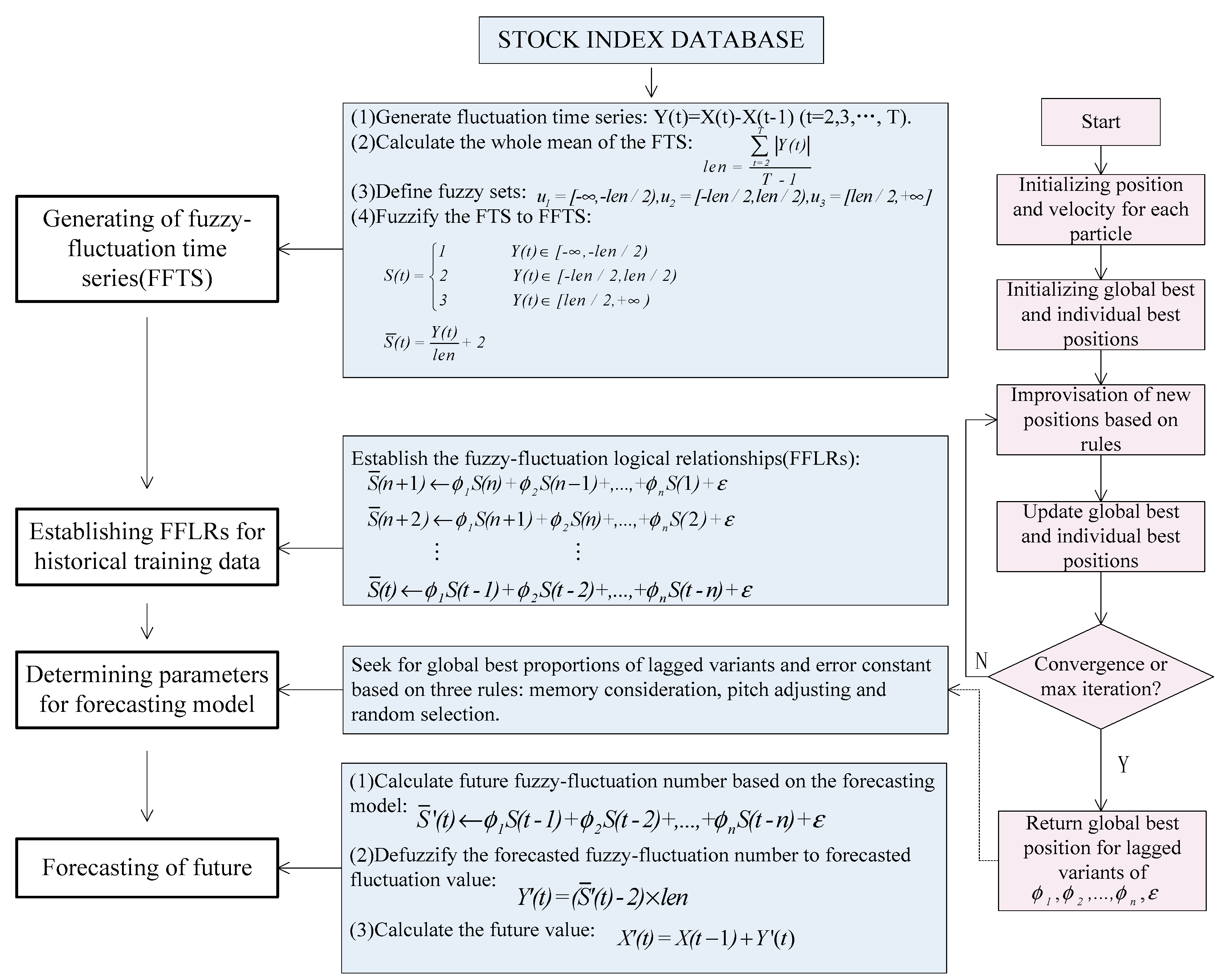
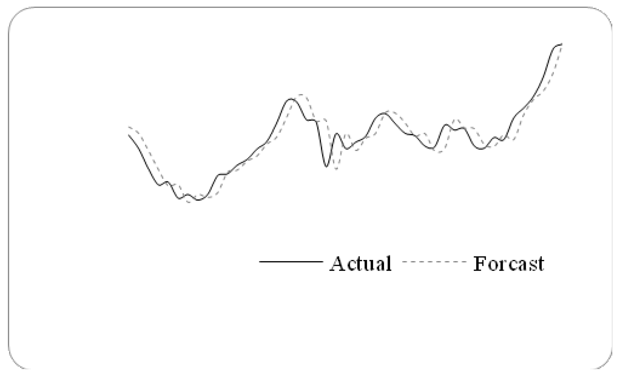
Figure 2.
Forecasting results from 1 November1999 to 30 December 1999.

Figure 3.
The stock marketfluctuation for TAIEX test dataset (1997–2005).
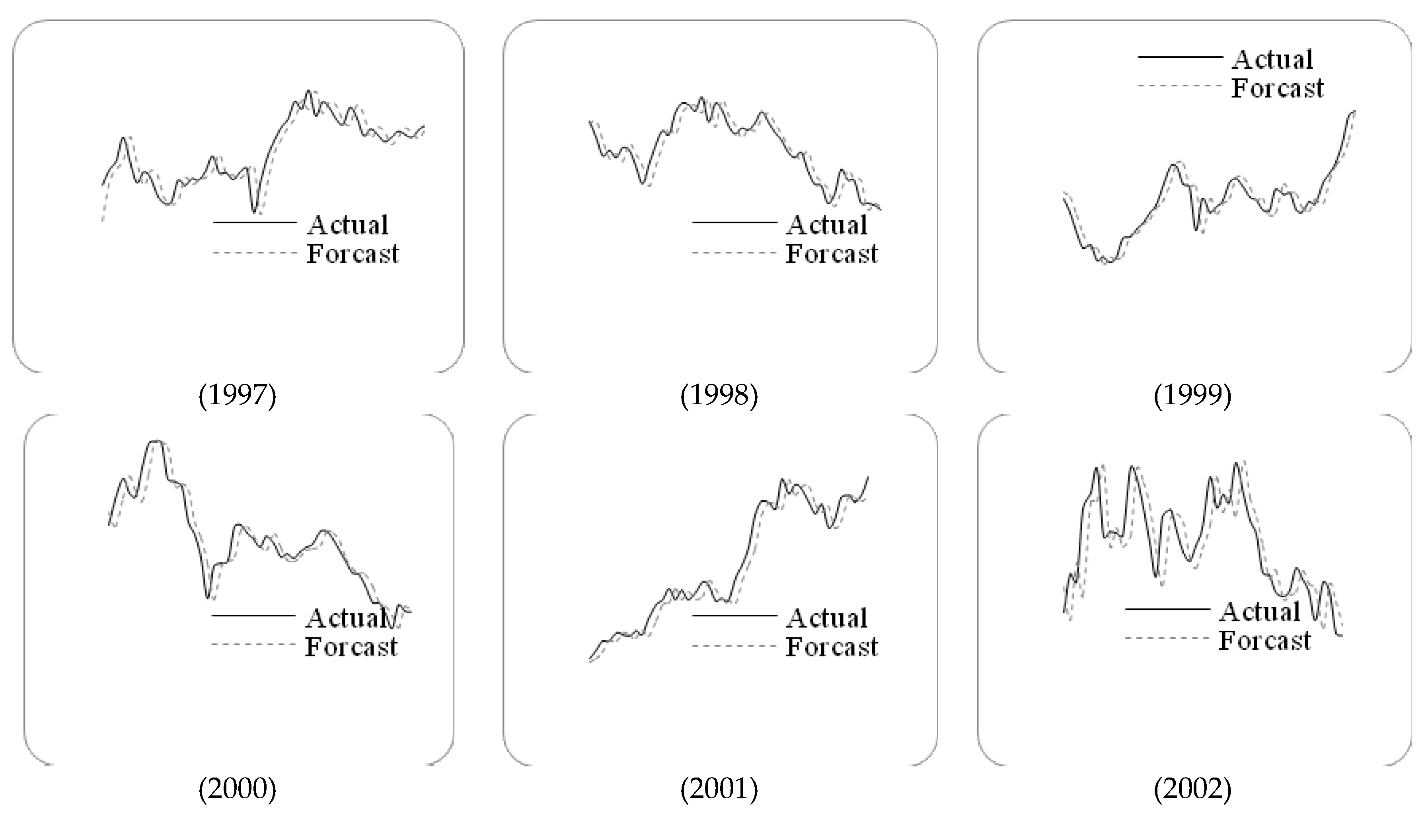
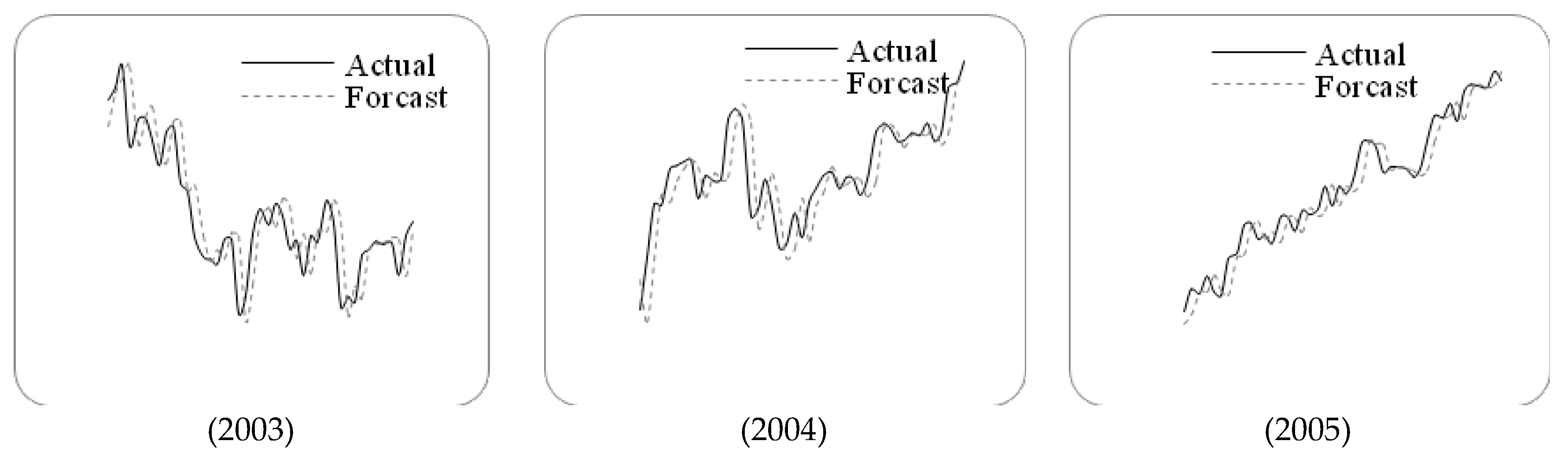
Table 1.
Global best parameters obtained using PSO for training dataset.
| ϕ1 | ϕ2 | ϕ3 | ϕ4 | ϕ5 | ϕ6 | E | RMSE |
|---|---|---|---|---|---|---|---|
| −0.1638 | 0.0803 | 0.1372 | −0.0321 | 0.0433 | 0.2546 | 1.4408 | 115.73 |
Table 2.
Forecasting results from 1 November1999 to 30 December 1999.
| Date (MM/DD/YYYY) | Actual | Forecast | (Forecast–Actual)2 | Date (MM/DD/YYYY) | Actual | Forecast | (Forecast–Actual)2 |
|---|---|---|---|---|---|---|---|
| 11/1/1999 | 7814.89 | 7869.35 | 2965.89 | 12/1/1999 | 7766.20 | 7705.59 | 3673.57 |
| 11/2/1999 | 7721.59 | 7825.35 | 10,766.14 | 12/2/1999 | 7806.26 | 7790.48 | 249.01 |
| 11/3/1999 | 7580.09 | 7704.00 | 15,353.69 | 12/3/1999 | 7933.17 | 7824.29 | 11,854.85 |
| 11/4/1999 | 7469.23 | 7573.21 | 10,811.84 | 12/4/1999 | 7964.49 | 7967.96 | 12.04 |
| 11/5/1999 | 7488.26 | 7460.24 | 785.12 | 12/6/1999 | 7894.46 | 7965.87 | 5099.39 |
| 11/6/1999 | 7376.56 | 7468.50 | 8452.96 | 12/7/1999 | 7827.05 | 7897.62 | 4980.12 |
| 11/8/1999 | 7401.49 | 7345.94 | 3085.80 | 12/8/1999 | 7811.02 | 7806.25 | 22.75 |
| 11/9/1999 | 7362.69 | 7400.03 | 1394.28 | 12/9/1999 | 7738.84 | 7823.68 | 7197.83 |
| 11/10/1999 | 7401.81 | 7379.30 | 506.70 | 12/10/1999 | 7733.77 | 7701.12 | 1066.02 |
| 11/11/1999 | 7532.22 | 7410.86 | 14,728.25 | 12/13/1999 | 7883.61 | 7718.38 | 27,300.95 |
| 11/15/1999 | 7545.03 | 7553.82 | 77.26 | 12/14/1999 | 7850.14 | 7921.86 | 5143.76 |
| 11/16/1999 | 7606.20 | 7569.42 | 1352.77 | 12/15/1999 | 7859.89 | 7862.87 | 8.88 |
| 11/17/1999 | 7645.78 | 7631.90 | 192.65 | 12/16/1999 | 7739.76 | 7857.12 | 13,773.37 |
| 11/18/1999 | 7718.06 | 7667.91 | 2515.02 | 12/17/1999 | 7723.22 | 7750.49 | 743.65 |
| 11/19/1999 | 7770.81 | 7750.58 | 409.25 | 12/18/1999 | 7797.87 | 7733.15 | 4188.68 |
| 11/20/1999 | 7900.34 | 7800.66 | 9936.10 | 12/20/1999 | 7782.94 | 7815.10 | 1034.27 |
| 11/22/1999 | 8052.31 | 7936.55 | 13,400.38 | 12/21/1999 | 7934.26 | 7781.74 | 23,262.35 |
| 11/23/1999 | 8046.19 | 8079.43 | 1104.90 | 12/22/1999 | 8002.76 | 7953.13 | 2463.14 |
| 11/24/1999 | 7921.85 | 8072.42 | 22,671.32 | 12/23/1999 | 8083.49 | 8060.46 | 530.38 |
| 11/25/1999 | 7904.53 | 7908.83 | 18.49 | 12/24/1999 | 8219.45 | 8119.70 | 9950.06 |
| 11/26/1999 | 7595.44 | 7912.20 | 100,336.90 | 12/27/1999 | 8415.07 | 8246.57 | 28,392.25 |
| 11/29/1999 | 7823.90 | 7576.21 | 61,350.34 | 12/28/1999 | 8448.84 | 8462.94 | 198.81 |
| 11/30/1999 | 7720.87 | 7823.06 | 10,442.80 | Root Mean Square Error(RMSE) | 99.31 | ||
Table 3.
Comparison of forecasting errors for different nth-orders (g=3).
| n | 1 | 2 | 3 | 4 | 5 | 6 | 7 | 8 | 9 | 10 |
|---|---|---|---|---|---|---|---|---|---|---|
| RMSE | 109.04 | 105.47 | 103.04 | 102.96 | 101.92 | 99.12 | 99.59 | 99.6 | 98.75 | 99 |
Table 4.
Comparison of forecasting errors for different linguistic sets (n=6).
| g | 3 | 5 | 7 | None |
|---|---|---|---|---|
| RMSE | 99.12 | 101.67 | 105.82 | 128.97 |
Table 5.
RMSEs of forecast errors for TAIEX 1997 to 2005.
| Year | 1997 | 1998 | 1999 | 2000 | 2001 | 2002 | 2003 | 2004 | 2005 |
|---|---|---|---|---|---|---|---|---|---|
| RMSE | 143.60 | 115.34 | 99.12 | 125.70 | 115.91 | 70.43 | 54.26 | 57.24 | 54.68 |
Table 6.
A comparison of RMSEs for different methods for forecasting the TAIEX1999.
| Methods | RMSE | S |
|---|---|---|
| Yu’s Method(2005) [36] | 145 | 1.62 ** |
| Hsieh et al.’s Method(2011) [51] | 94 | −0.32 |
| Chang et al.’s Method(2011) [48] | 100 | 0.11 |
| Cheng et al.’s Method(2013) [50] | 103 | 0.34 |
| Chen et al.’s Method(2013) [49] | 102.11 | 0.21 |
| Chen and Chen’s Method(2015) [11] | 103.9 | 0.36 |
| Chen and Chen’s Method(2015) [10] | 92 | −0.42 |
| Zhao et al.’s Method(2016) [27] | 110.85 | 1.08 |
| The Proposed Method | 99.12 | - |
** The proposed method has better predictive accuracy than the method at the 5% significance level.
Table 7.
RMSEs of the forecast errors for year 2015 of DAX30.
| Year | Yu (2005) [36] | Cheng et al. (2008) [37] | Wang et al. (2013) [25] | Rubio et al. (2017) [13] | Proposed Model |
|---|---|---|---|---|---|
| RMSE | 172.69 | 170.56 | 376.80 | 153.15 | 159.22 |
| S | 1.31 | 1.23 | 3.68 ** | −0.26 | - |
** The proposed method has better predictive accuracy than the method at the 5% significancelevel.
Table 8.
RMSEs of forecast errors for SHSECI from 2007 to 2015.
| Year | 2007 | 2008 | 2009 | 2010 | 2011 | 2012 | 2013 | 2014 | 2015 |
|---|---|---|---|---|---|---|---|---|---|
| RMSE | 113.11 | 55.28 | 49.59 | 45.73 | 28.45 | 25.05 | 19.86 | 41.44 | 59.5 |
© 2017 by the authors. Licensee MDPI, Basel, Switzerland. This article is an open access article distributed under the terms and conditions of the Creative Commons Attribution (CC BY) license (http://creativecommons.org/licenses/by/4.0/).
Share and Cite
MDPI and ACS Style
Jia, J.; Zhao, A.; Guan, S. Forecasting Based on High-Order Fuzzy-Fluctuation Trends and Particle Swarm Optimization Machine Learning. Symmetry 2017, 9, 124. https://doi.org/10.3390/sym9070124
AMA Style
Jia J, Zhao A, Guan S. Forecasting Based on High-Order Fuzzy-Fluctuation Trends and Particle Swarm Optimization Machine Learning. Symmetry. 2017; 9(7):124. https://doi.org/10.3390/sym9070124
Chicago/Turabian StyleJia, Jingyuan, Aiwu Zhao, and Shuang Guan. 2017. "Forecasting Based on High-Order Fuzzy-Fluctuation Trends and Particle Swarm Optimization Machine Learning" Symmetry 9, no. 7: 124. https://doi.org/10.3390/sym9070124
Note that from the first issue of 2016, this journal uses article numbers instead of page numbers. See further details here.