
A Novel Neutrosophic Weighted Extreme Learning Machine for Imbalanced Data Set


1
Department of Electrical and Electronics Engineering, Technology Faculty, Firat University, 23119 Elazig, Turkey
2
Department of Computer Science, University of Illinois at Springfield, Springfield, IL 62703, USA
3
Department of Mathematics and Sciences, University of New Mexico, Gallup, NM 87301, USA
*
Author to whom correspondence should be addressed.
Symmetry 2017, 9(8), 142; https://doi.org/10.3390/sym9080142
Submission received: 23 June 2017
/
Revised: 31 July 2017
/
Accepted: 1 August 2017
/
Published: 3 August 2017
(This article belongs to the Special Issue Neutrosophic Theories Applied in Engineering)
Abstract
:Extreme learning machine (ELM) is known as a kind of single-hidden layer feedforward network (SLFN), and has obtained considerable attention within the machine learning community and achieved various real-world applications. It has advantages such as good generalization performance, fast learning speed, and low computational cost. However, the ELM might have problems in the classification of imbalanced data sets. In this paper, we present a novel weighted ELM scheme based on neutrosophic set theory, denoted as neutrosophic weighted extreme learning machine (NWELM), in which neutrosophic c-means (NCM) clustering algorithm is used for the approximation of the output weights of the ELM. We also investigate and compare NWELM with several weighted algorithms. The proposed method demonstrates advantages to compare with the previous studies on benchmarks.
1. Introduction
Extreme learning machine (ELM) was put forward in 2006 by Huang et al. [1] as a single-hidden layer feedforward network (SLFN). The hidden layer parameters of ELM are arbitrarily initialized and output weights are determined by utilizing the least squares algorithm. Due to this characteristic, ELM has fast learning speed, better performance and efficient computation cost [1,2,3,4], and has, as a result, been applied in different areas.
However, ELM suffers from the presence of irrelevant variables in the large and high dimensional real data set [2,5]. The unbalanced data set problem occurs in real applications such as text categorization, fault detection, fraud detection, oil-spills detection in satellite images, toxicology, cultural modeling, and medical diagnosis [6]. Many challenging real problems are characterized by imbalanced training data in which at least one class is under-represented relative to others.
The problem of imbalanced data is often associated with asymmetric costs of misclassifying elements of different classes. In addition, the distribution of the test data set might differ from that of the training samples. Class imbalance happens when the number of samples in one class is much more than that of the other [7]. The methods aiming to tackle the problem of imbalance can be classified into four groups such as algorithmic based methods, data based methods, cost-sensitive methods and ensembles of classifiers based methods [8]. In algorithmic based approaches, the minority class classification accuracy is improved by adjusting the weights for each class [9]. Re-sampling methods can be viewed in the data based approaches where these methods did not improve the classifiers [10]. The cost-sensitive approaches assign various cost values to training samples of the majority class and the minority class, respectively [11]. Recently, ensembles based methods have been widely used in classification of imbalanced data sets [12]. Bagging and boosting methods are the two popular ensemble methods.
The problem of class imbalance has received much attention in the literature [13]. Synthetic minority over–sampling technique (SMOTE) [9] is known as the most popular re-sampling method that uses pre-processing for obtaining minority class instances artificially. For each minority class sample, SMOTE creates a new sample on the line joining it to the nearest minority class neighbor. Borderline SMOTE [14], SMOTE-Boost [15], and modified SMOTE [14] are some of the improved variants of the SMOTE algorithm. In addition, an oversampling method was proposed that identifies some minority class samples that are hard to classify [16]. Another oversampling method was presented that uses bagging with oversampling [17]. In [18], authors opted to use double ensemble classifier by combining bagging and boosting. In [19], authors combined sampling and ensemble techniques to improve the classification performance for skewed data. Another method, namely random under sampling (RUS), was proposed that removes the majority class samples randomly until the training set becomes balanced [19]. In [20], authors proposed an ensemble of an support vector machine (SVM) structure with boosting (Boosting-SVM), where the minority class classification accuracy was increased compared to pure SVM. In [21], a cost sensitive approach was proposed where k-nearest neighbors (k-NN) classifier was adopted. In addition, in [22], an SVM based cost sensitive approach was proposed for class imbalanced data classification. Decision trees [23] and logistic regression [24] based methods were also proposed in order to handle with the imbalanced data classification.
An ELM classifier trained with an imbalanced data set can be biased towards the majority class and obtain a high accuracy on the majority class by compromising minority class accuracy. Weighted ELM (WELM) was employed to alleviate the ELM’s classification deficiency on imbalanced data sets, and which can be seen as one of the cost-proportionate weighted sampling methods [25]. ELM assigns the same misclassification cost value to all data points such as positive and negative samples in a two-class problem. When the number of negative samples is much larger than that of the number of positive samples or vice versa, assigning the same misclassification cost value to all samples can be seen one of the drawbacks of traditional ELM. A straightforward solution is to obtain misclassification cost values adaptively according to the class distribution, in the form of a weight scheme inversely proportional to the number of samples in the class.
In [7], the authors proposed a weighted online sequential extreme learning machine (WOS-ELM) algorithm for alleviating the imbalance problem in chunk-by-chunk and one-by-one learning. A weight setting was selected in a computationally efficient way. Weighted Tanimoto extreme learning machine (T-WELM) was used to predict chemical compound biological activity and other data with discrete, binary representation [26]. In [27], the authors presented a weight learning machine for a SLFN to recognize handwritten digits. Input and output weights were globally optimized with the batch learning type of least squares. Features were assigned into the prescribed positions. Another weighted ELM algorithm, namely ESOS-ELM, was proposed by Mirza et al. [28], which was inspired from WOS-ELM. ESOS-ELM aims to handle class imbalance learning (CIL) from a concept-drifting data stream. Another ensemble-based weighted ELM method was proposed by Zhang et al. [29], where the weight of each base learner in the ensemble is optimized by differential evolution algorithm. In [30], the authors further improved the re-sampling strategy inside Over-sampling based online bagging (OOB) and Under-sampling based online bagging (UOB) in order to learn class imbalance.
Although much awareness of the imbalance has been raised, many of the key issues remain unresolved and encountered more frequently in massive data sets. How to determine the weight values is key to designing WELM. Different situations such as noises and outlier data should be considered.
The noises and outlier data in a data set can be treated as a kind of indeterminacy. Neutrosophic set (NS) has been successfully applied for indeterminate information processing, and demonstrates advantages to deal with the indeterminacy information of data and is still a technique promoted for data analysis and classification application. NS provides an efficient and accurate way to define imbalance information according to the attributes of the data.
In this study, we present a new weighted ELM scheme using neutrosophic c-means (NCM) clustering to overcome the ELM’s drawbacks in highly imbalanced data sets. A novel clustering algorithm NCM was proposed for data clustering [31,32]. NCM is employed to determine a sample’s belonging, noise, and indeterminacy memberships, and is then used to compute a weight value for that sample [31,32,33]. A weighted ELM is designed using the weights from NCM and utilized for imbalanced data set classification.
2. Proposed Method
2.1. Extreme Learning Machine
Backpropagation, which is known as gradient-based learning method, suffers from slow convergence speed. In addition, stuck in the local minimum can be seen as another disadvantage of a gradient-based learning algorithm. ELM was proposed by Huang et al. [1] as an alternative method that overcomes the shortcomings of gradient-based learning methods. The ELM was designed as an SLFN, where the input weights and hidden biases are selected randomly. These weights do not need to be adjusted during the training process. The output weights are determined analytically with Moore–Penrose generalized inverse of the hidden-layer output matrix.
Mathematically speaking, the output of the ELM with L hidden nodes and activation function g(·) can be written as:
where is the jth input data, is the weight vector, is the output weight vector, is the bias of the jth hidden node and is the ith output node and N shows the number of samples. If ELM learns these N samples with 0 error, then Equation (1) can be updated as follows:
where shows the actual output vector. Equation (2) can be written compactly as shown in Equation (3):
where is the hidden-layer output matrix. Thus, the output weight vector can be calculated analytically with Moore–Penrose generalized inverse of the hidden-layer output matrix as shown in Equation (4):
where is the Moore–Penrose generalized inverse of matrix H.
2.2. Weighted Extreme Learning Machine
Let us consider a training data set belonging to two classes, where and are the class labels. In binary classification, is either or . Then, a diagonal matrix is considered, where each of them is associated with a training sample . The weighting procedure generally assigns larger to , which comes from the minority class.
An optimization problem is employed to maximize the marginal distance and to minimize the weighted cumulative error as:
Furthermore:
where , is the error vector and is the feature mapping vector in the hidden layer with respect to , and . By using the Lagrage multiplier and Karush–Kuhn–Tucker theorem, the dual optimization problem can be solved. Thus, hidden layer’s output weight vector becomes can be derived from Equation (7) regarding left pseudo-inverse or right pseudo-inverse. When presented data with small size, right pseudo-inverse is recommended because it involves the inverse of an matrix. Otherwise, left pseudo-inverse is more suitable since it is much easier to compute matrix inversion of size when L is much smaller than N:
In the weighted ELM, the authors adopted two different weighting schemes. In the first one, the weights for the minority and majority classes are calculated as:
and, for the second one, the related weights are calculated as:
The readers may refer to [25] for detail information about determination of the weights.
2.3. Neutrosophic Weighted Extreme Learning Machine
Weighted ELM assigns the same weight value to all samples in the minority class and another same weight value to all samples in the majority class. Although this procedure works quite well in some imbalanced data sets, assigning the same weight value to all samples in a class may not be a good choice for data sets that have noise and outlier samples. In other words, to deal with noise and outlier data samples in an imbalanced data set, different weight values are needed for each sample in each class that reflects the data point’s significance in its class. Therefore, we present a novel method to determine the significance of each sample in its class. NCM clustering can determine a sample’s belonging, noise and indeterminacy memberships, which can then be used in order to compute a weight value for that sample.
Guo and Sengur [31] proposed the NCM clustering algorithms based on the neutrosophic set theorem [34,35,36,37]. In NCM, a new cost function was developed to overcome the weakness of the Fuzzy c-Means (FCM) method on noise and outlier data points. In the NCM algorithm, two new types of rejection were developed for both noise and outlier rejections. The objective function in NCM is given as follows:
where m is a constant. For each point i, the is the mean of two centers. , and are the membership values belonging to the determinate clusters, boundary regions and noisy data set. , , :
Thus, the related membership functions are calculated as follows:
where shows the center of cluster j, , , and are the weight factors and is a regularization factor which is data dependent [31]. Under the above definitions, every input sample in each minority and majority class is associated with a triple , , . While the larger means that the sample belongs to the labeled class with a higher probability, the larger means that the sample is indeterminate with a higher probability. Finally, the larger means that the sample is highly probable to be a noise or outlier data.
After clustering procedure is applied in NCM, the weights for each sample of minority and majority classes are obtained as follows:
where is the ratio of the number of samples in the majority class to the number of the samples in the minority class.
The algorithm of the neutrosophic weighted extreme learning machine (NWELM) is composed of four steps. The first step necessitates applying the NCM algorithm based on the pre-calculated cluster centers, according to the class labels of the input samples. Thus, the T, I and F membership values are determined for the next step. The related weights are calculated from the determined T, I and F membership values in the second step of the algorithm.
In Step 3, the ELM parameters are tuned and samples and weights are fed into the ELM in order to calculate the H matrix. The hidden layer weight vector is calculated according to the H, W and class labels. Finally, the determination of the labels of the test data set is accomplished in the final step of the algorithm (Step 4).
The neutrosophic weighted extreme learning machine (NWELM) algorithm is given as following:
- Input:
- Labelled training data set.
- Output:
- Predicted class labels.
- Step 1:
- Initialize the cluster centers according to the labelled data set and run NCM algorithm in order to obtain the T, I and F value for each data point.
- Step 2:
- Step 3:
- Step 4:
- Calculate the labels of test data set based on .
3. Experimental Results
The geometric mean () is used to evaluate the performance of the proposed NWELM method. The is computed as follows:
where R denotes the recall rate and , denotes true-negative and false-positive detections, respectively. values are in the range of [0–1] and it represents the square root of positive class accuracy and negative class accuracy. The performance evaluation of NWELM classifier is tested on both toy data sets and real data sets, respectively. The five-fold cross-validation method is adopted in the experiments. In the hidden node of the NWELM, the radial basis function (RBF) kernel is considered. A grid search of the trade-off constant C on {, , …, , } and the number of hidden nodes L on {10, 20, …, 990, 2000} was conducted in seeking the optimal result using five-fold cross-validation. For real data sets, a normalization of the input attributes into [, 1] is considered. In addition, for NCM, the following parameters are chosen such as , , , respectively, which were obtained by means of trial and error. The parameter of NCM method is also searched on {, , …, , }.
3.1. Experiments on Artificial Data Sets
Four two-class artificial imbalance data sets were used to evaluate the classification performance of the proposed NWELM scheme. The illustration of the data sets is shown in Figure 1 [38]. The decision boundary between classes is complicated. In Figure 1a, we illustrate the first artificial data set that follows a uniform distribution. As can be seen, the red circles of Figure 1a belong to the minority class, with the rest of the data samples shown by blue crosses as the majority class. The second imbalance data set, namely Gaussian-1, is obtained using two Gaussian distributions with a 1:9 ratio of samples as shown in Figure 1b. While the red circles illustrate the minority class, the blue cross samples show the majority class.
Another Gaussian distribution-based imbalance data set, namely Gaussian-2, is given in Figure 1c. This data set consists of nine Gaussian distributions with the same number of samples arranged in a grid. The red circle samples located in the middle belong to the minority class while the blue cross samples belong to the majority class. Finally, Figure 1d shows the last artificial imbalance data set. It is known as a complex data set because it has a 1:9 ratio of samples for the minority and majority classes.
Table 1 shows the achieved by the two methods on these four data sets in ten independent runs. For Gaussian-1, Gaussian-2 and the Uniform artificial data sets, the proposed NWELM method yields better results when compared to the weighted ELM scheme; however, for the Complex artificial data sets, the weighted ELM method achieves better results. The better resulting cases are shown in bold text. It is worth mentioning that, for the Gaussian-2 data set, NWELM achieves a higher across all trials.
3.2. Experiments on Real Data Set
In this section, we test the achievement of the proposed NWELM method on real data sets [39]. A total of 21 data sets with different numbers of features, training and test samples, and imbalance ratios are shown in Table 2. The selected data sets can be categorized into two classes according to their imbalance ratios. The first class has the imbalance ratio range of 0 to 0.2 and contains yeast-1-2-8-9_vs_7, abalone9_18, glass-0-1-6_vs_2, vowel0, yeast-0-5-6-7-9_vs_4, page-blocks0, yeast3, ecoli2, new-thyroid1 and the new-thyroid2 data sets.
On the other hand, second class contains the data sets, such as ecoli1, glass-0-1-2-3_vs_4-5-6, vehicle0, vehicle1, haberman, yeast, glass0, iris0, pima, wisconsin and glass1, that have imbalance ratio rates between 0.2 and 1.
The comparison results of the proposed NWELM with the weighted ELM, unweighted ELM and SVM are given in Table 3. As the weighted ELM method used a different weighting scheme (, ), in our comparisons, we used the higher value. As can be seen in Table 3, the NWELM method yields higher values for 17 of the imbalanced data sets. For three of the data sets, both methods yield the same . Just for the page-blocks0 data set, the weighted ELM method yielded better results. It is worth mentioning that the NWELM method achieves 100% values for four data sets (vowel0, new-thyroid1, new-thyroid2, iris0). In addition, NWELM produced higher values than SVM for all data sets.
The obtained results were further evaluated by area under curve (AUC) values [40]. In addition, we compared the proposed method with unweighted ELM, weighted ELM and SVM based on the achieved AUC values as tabulated in Table 4. As seen in Table 4, for all examined data sets, our proposal’s AUC values were higher than the compared other methods. For further comparisons of the proposed method with unweighted ELM, weighted ELM and SVM methods appropriately, statistical tests on AUC results were considered. The paired t-test was chosen [41]. The paired t-test results between each compared method and the proposed method for AUC was tabulated in Table 5 in terms of p-value. In Table 5, the results showing a significant advantage to the proposed method were shown in bold–face where p-values are equal or smaller than 0.05. Therefore, the proposed method performed better than the other methods in 39 tests out of 63 tests when each data set and pairs of methods are considered separately.
Another statistical test, namely the Friedman aligned ranks test, has been applied to compare the obtained results based on AUC values [42]. This test is a non-parametric test and the Holm method was chosen as the post hoc control method. The significance level was assigned 0.05. The statistics were obtained with the STAC tool [43] and recorded in Table 6. According to these results, the highest rank value was obtained by the proposed NWELM method and SVM and WELM rank values were greater than the ELM. In addition, the comparison’s statistics, adjusted p-values and hypothesis results were given in Table 6.
We further compared the proposed NWELM method with two ensemble-based weighted ELM methods on 12 data sets [29]. The obtained results and the average classification values are recorded in Table 7. The best classification result for each data set is shown in bold text. A global view on the average classification performance shows that the NWELM yielded the highest average value against both the ensemble-based weighted ELM methods. In addition, the proposed NWELM method evidently outperforms the other two compared algorithms in terms of in 10 out of 12 data sets, with the only exceptions being the yeast3 and glass2 data sets.
As can be seen through careful observation, the NWELM method has not significantly improved the performance in terms of the glass1, haberman, yeast1_7 and abalone9_18 data sets, but slightly outperforms both ensemble-based weighted ELM methods.
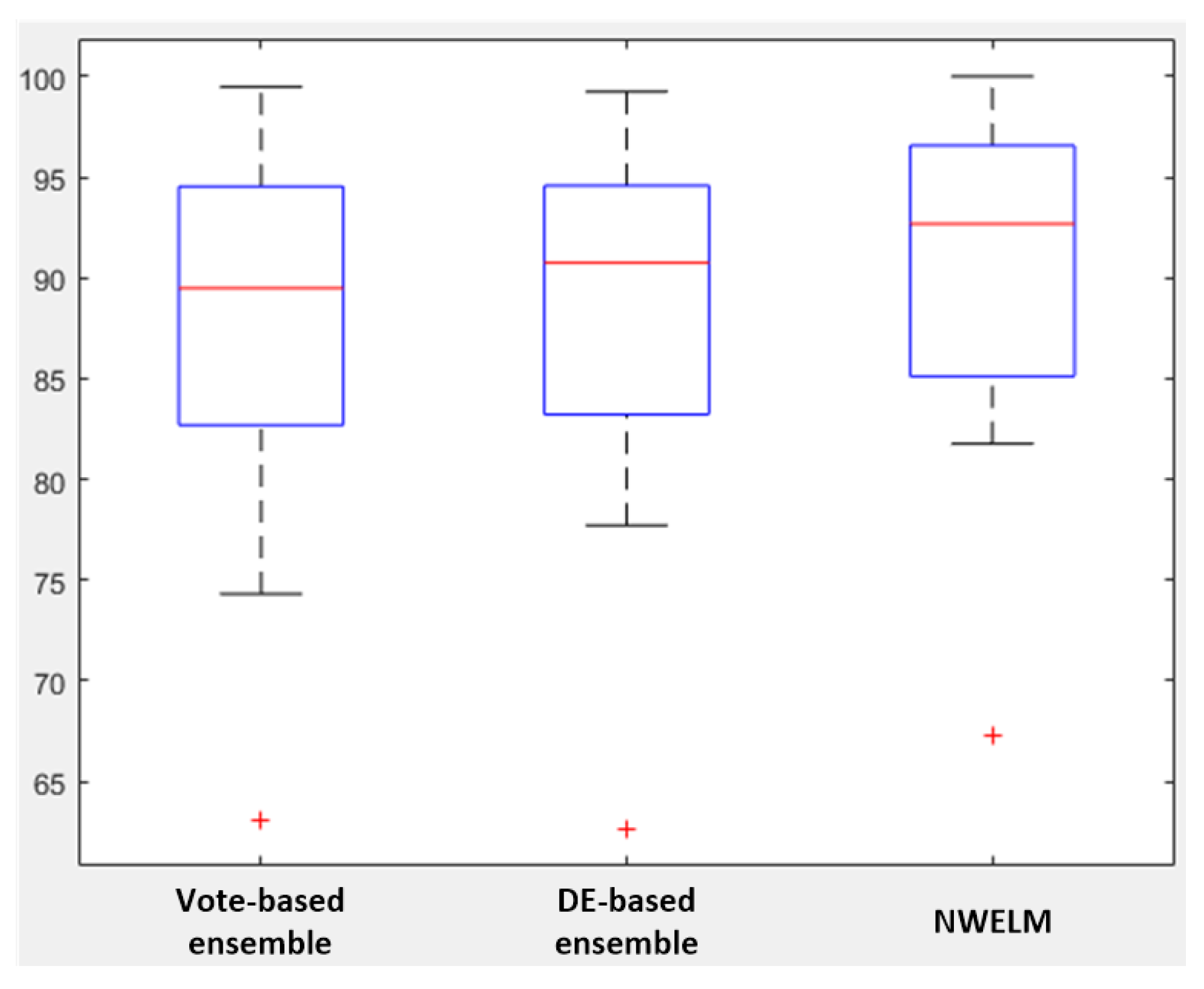
A box plots illustration of the compared methods is shown in Figure 2. The box generated by the NWELM is shorter than the boxes generated by the compared vote-based ensemble and differential evolution (DE)- based ensemble methods. The dispersion degree of NWELM method is relatively low. It is worth noting that the box plots of all methods consider the of the haberman data set as an exception. Finally, the box plot determines the proposed NWELM method to be more robust when compared to the ensemble-based weighted ELM methods.
4. Conclusions
In this paper, we propose a new weighted ELM model based on neutrosophic clustering. This new weighting scheme introduces true, indeterminacy and falsity memberships of each data point into ELM. Thus, we can remove the effect of noises and outliers in the classification stage and yield better classification results. Moreover, the proposed NWELM scheme can handle the problem of class imbalance more effectively. In the evaluation experiments, we compare the performance of the NWELM method with weighted ELM, unweighted ELM, and two ensemble-based weighted ELM methods. The experimental results demonstrate the NEWLM to be more effective than the compared methods for both artificial and real binary imbalance data sets. In the future, we are planning to extend our study to multiclass imbalance learning.
Author Contributions
Abdulkadir Sengur provided the idea of the proposed method. Yanhui Guo and Florentin Smarandache proved the theorems. Yaman Akbulut analyzed the model’s application. Abdulkadir Sengur, Yanhui Guo, Yaman Akbulut, and Florentin Smarandache wrote the paper.
Conflicts of Interest
The authors declare no conflict of interest.
References
- Huang, G.B.; Zhu, Q.Y.; Siew, C.K. Extreme learning machine: Theory and applications. Neurocomputing 2006, 70, 489–501. [Google Scholar] [CrossRef]
- Miche, Y.; Van Heeswijk, M.; Bas, P.; Simula, O.; Lendasse, A. TROP-ELM: A double-regularized ELM using LARS and Tikhonov regularization. Neurocomputing 2011, 74, 2413–2421. [Google Scholar] [CrossRef]
- Deng, W.; Zheng, Q.; Chen, L. Regularized Extreme Learning Machine. In Proceedings of the 2009 IEEE Symposium on Computational Intelligence and Data Mining, Nashville, TN, USA, 30 March–2 April 2009; pp. 389–395. [Google Scholar]
- MartíNez-MartíNez, J.M.; Escandell-Montero, P.; Soria-Olivas, E.; MartíN-Guerrero, J.D.; Magdalena-Benedito, R.; GóMez-Sanchis, J. Regularized extreme learning machine for regression problems. Neurocomputing 2011, 74, 3716–3721. [Google Scholar] [CrossRef]
- Miche, Y.; Sorjamaa, A.; Bas, P.; Simula, O.; Jutten, C.; Lendasse, A. OP-ELM: Optimally pruned extreme learning machine. IEEE Trans. Neural Netw. 2010, 21, 158–162. [Google Scholar] [CrossRef] [PubMed]
- Vajda, S.; Fink, G.A. Strategies for Training Robust Neural Network Based Digit Recognizers on Unbalanced Data Sets. In Proceedings of the 2010 International Conference on Frontiers in Handwriting Recognition (ICFHR), Kolkata, India, 16–18 November 2010; pp. 148–153. [Google Scholar]
- Mirza, B.; Lin, Z.; Toh, K.A. Weighted online sequential extreme learning machine for class imbalance learning. Neural Process. Lett. 2013, 38, 465–486. [Google Scholar] [CrossRef]
- Beyan, C.; Fisher, R. Classifying imbalanced data sets using similarity based hierarchical decomposition. Pattern Recognit. 2015, 48, 1653–1672. [Google Scholar] [CrossRef]
- Chawla, N.V.; Bowyer, K.W.; Hall, L.O.; Kegelmeyer, W.P. SMOTE: Synthetic minority over-sampling technique. J. Artif. Intell. Res. 2002, 16, 321–357. [Google Scholar]
- Pazzani, M.; Merz, C.; Murphy, P.; Ali, K.; Hume, T.; Brunk, C. Reducing Misclassification Costs. In Proceedings of the Eleventh International Conference on Machine Learning, New Brunswick, NJ, USA, 10–13 July 1994; pp. 217–225. [Google Scholar]
- Japkowicz, N. The Class Imbalance Problem: Significance and Strategies. In Proceedings of the 2000 International Conference on Artificial Intelligence (IC-AI’2000), Las Vegas, NV, USA, 26–29 June 2000. [Google Scholar]
- Galar, M.; Fernandez, A.; Barrenechea, E.; Bustince, H.; Herrera, F. A Review on Ensembles for the Class Imbalance Problem: Bagging-, Boosting-, and Hybrid-Based Approaches. IEEE Trans. Syst. Man Cybern. Part C (Appl. Rev.) 2012, 42, 463–484. [Google Scholar] [CrossRef]
- He, H.; Garcia, E.A. Learning from imbalanced data. IEEE Trans. Knowl. Data Eng. 2009, 21, 1263–1284. [Google Scholar]
- Hu, S.; Liang, Y.; Ma, L.; He, Y. MSMOTE: Improving Classification Performance when Training Data is Imbalanced. In Proceedings of the Second International Workshop on Computer Science and Engineering (WCSE’09), Qingdao, China, 28–30 October 2009; IEEE: Washington, DC, USA, 2009; Volume 2, pp. 13–17. [Google Scholar]
- Chawla, N.; Lazarevic, A.; Hall, L.; Bowyer, K. SMOTEBoost: Improving Prediction of the Minority Class in Boosting. In Proceedings of the 7th European Conference on Principles and Practice of Knowledge Discovery in Databases, Cavtat-Dubrovnik, Croatia, 22–26 September 2003; pp. 107–119. [Google Scholar]
- Barua, S.; Islam, M.M.; Yao, X.; Murase, K. MWMOTE–majority weighted minority oversampling technique for imbalanced data set learning. IEEE Trans. Knowl. Data Eng. 2014, 26, 405–425. [Google Scholar] [CrossRef]
- Radivojac, P.; Chawla, N.V.; Dunker, A.K.; Obradovic, Z. Classification and knowledge discovery in protein databases. J. Biomed. Inf. 2004, 37, 224–239. [Google Scholar] [CrossRef] [PubMed]
- Liu, X.Y.; Wu, J.; Zhou, Z.H. Exploratory undersampling for class-imbalance learning. IEEE Trans. Syst. Man Cybern. Part B (Cybern.) 2009, 39, 539–550. [Google Scholar]
- Seiffert, C.; Khoshgoftaar, T.M.; Van Hulse, J.; Napolitano, A. RUSBoost: A hybrid approach to alleviating class imbalance. IEEE Trans. Syst. Man Cybern. Part A Syst. Hum. 2010, 40, 185–197. [Google Scholar] [CrossRef]
- Wang, B.X.; Japkowicz, N. Boosting support vector machines for imbalanced data sets. Knowl. Inf. Syst. 2010, 25, 1–20. [Google Scholar] [CrossRef]
- Tan, S. Neighbor-weighted k-nearest neighbor for unbalanced text corpus. Expert Syst. Appl. 2005, 28, 667–671. [Google Scholar] [CrossRef]
- Fumera, G.; Roli, F. Cost-sensitive learning in support vector machines. In Proceedings of the VIII Convegno Associazione Italiana per l’Intelligenza Artificiale, Siena, Italy, 10–13 September 2002. [Google Scholar]
- Drummond, C.; Holte, R.C. Exploiting the cost (in) sensitivity of decision tree splitting criteria. In Proceedings of the Seventeenth International Conference on Machine Learning (ICML-2000), Stanford, CA, USA, 29 June–2 July 2000; Morgan Kaufmann Publishers Inc.: San Francisco, CA, USA, 2000; Volume 1, pp. 239–246. [Google Scholar]
- Williams, D.P.; Myers, V.; Silvious, M.S. Mine classification with imbalanced data. IEEE Geosci. Remote Sens. Lett. 2009, 6, 528–532. [Google Scholar] [CrossRef]
- Zong, W.; Huang, G.B.; Chen, Y. Weighted extreme learning machine for imbalance learning. Neurocomputing 2013, 101, 229–242. [Google Scholar] [CrossRef]
- Czarnecki, W.M. Weighted tanimoto extreme learning machine with case study in drug discovery. IEEE Comput. Intell. Mag. 2015, 10, 19–29. [Google Scholar] [CrossRef]
- Man, Z.; Lee, K.; Wang, D.; Cao, Z.; Khoo, S. An optimal weight learning machine for handwritten digit image recognition. Signal Process. 2013, 93, 1624–1638. [Google Scholar] [CrossRef]
- Mirza, B.; Lin, Z.; Liu, N. Ensemble of subset online sequential extreme learning machine for class imbalance and concept drift. Neurocomputing 2015, 149, 316–329. [Google Scholar] [CrossRef]
- Zhang, Y.; Liu, B.; Cai, J.; Zhang, S. Ensemble weighted extreme learning machine for imbalanced data classification based on differential evolution. Neural Comput. Appl. 2016, 1–9. [Google Scholar] [CrossRef]
- Wang, S.; Minku, L.L.; Yao, X. Resampling-based ensemble methods for online class imbalance learning. IEEE Trans. Knowl. Data Eng. 2015, 27, 1356–1368. [Google Scholar] [CrossRef]
- Guo, Y.; Sengur, A. NCM: Neutrosophic c-means clustering algorithm. Pattern Recognit. 2015, 48, 2710–2724. [Google Scholar] [CrossRef]
- Guo, Y.; Sengur, A. NECM: Neutrosophic evidential c-means clustering algorithm. Neural Comput. Appl. 2015, 26, 561–571. [Google Scholar] [CrossRef]
- Guo, Y.; Sengur, A. A novel 3D skeleton algorithm based on neutrosophic cost function. Appl. Soft Comput. 2015, 36, 210–217. [Google Scholar] [CrossRef]
- Smarandache, F. A Unifying Field in Logics: Neutrosophic Logic. Neutrosophic Probability, Neutrosophic Set. In Proceedings of the 2000 Western Section Meeting (Meeting #951), Preliminary Report, Santa Barbara, CA, USA, 11–12 March 2000; Volume 951, pp. 11–12. [Google Scholar]
- Smarandache, F. Introduction to Neutrosophic Measure, Neutrosophic Integral, and Neutrosophic Probability; Sitech: Craiova, Romania, 2013. [Google Scholar]
- Smarandache, F. Neutrosophy, Neutrosophic Probability, Set, and Logic; American Research Press: Rehoboth, DE, USA, 1998; p. 105. [Google Scholar]
- Smarandache, F. A Unifying Field in Logics: Neutrosophic Logic. Neutrosophy, Neutrosophic Set, Neutrosophic Probability: Neutrsophic Logic. Neutrosophy, Neutrosophic Set, Neutrosophic Probability; Infinite Study: Ann Arbor, MI, USA, 2005; ISBN 9781599730806. [Google Scholar]
- Ng, W.W.; Hu, J.; Yeung, D.S.; Yin, S.; Roli, F. Diversified sensitivity-based undersampling for imbalance classification problems. IEEE Trans. Cybern. 2015, 45, 2402–2412. [Google Scholar] [CrossRef] [PubMed]
- Alcalá-Fdez, J.; Fernández, A.; Luengo, J.; Derrac, J.; García, S.; Sánchez, L.; Herrera, F. Keel data-mining software tool: Data set repository, integration of algorithms and experimental analysis framework. J. Mult. Valued Log. Soft Comput. 2011, 17, 255–287. [Google Scholar]
- Huang, J.; Ling, C.X. Using AUC and accuracy in evaluating learning algorithms. IEEE Trans. Knowl. Data Eng. 2005, 17, 299–310. [Google Scholar] [CrossRef]
- Demšar, J. Statistical comparisons of classifiers over multiple data sets. J. Mach. Learn. Res. 2006, 7, 1–30. [Google Scholar]
- Hodges, J., Jr.; Lehmann, E. Rank methods for combination of independent experiments in analysis of variance. In Selected Works of E.L. Lehmann; Selected Works in Probability and Statistics; Springer: Boston, MA, USA, 2012; pp. 403–418. [Google Scholar]
- Rodríguez-Fdez, I.; Canosa, A.; Mucientes, M.; Bugarín, A. STAC: A Web Platform for the Comparison of Algorithms Using Statistical Tests. In Proceedings of the 2015 IEEE International Conference on Fuzzy Systems (FUZZ-IEEE), Istanbul, Turkey, 2–5 August 2015; pp. 1–8. [Google Scholar]
Figure 1.
Four 2-dimensional artificial imbalance data sets (, ): (a) uniform; (b) gaussian-1; (c) gaussian-2; and (d) complex.
Figure 1.
Four 2-dimensional artificial imbalance data sets (, ): (a) uniform; (b) gaussian-1; (c) gaussian-2; and (d) complex.
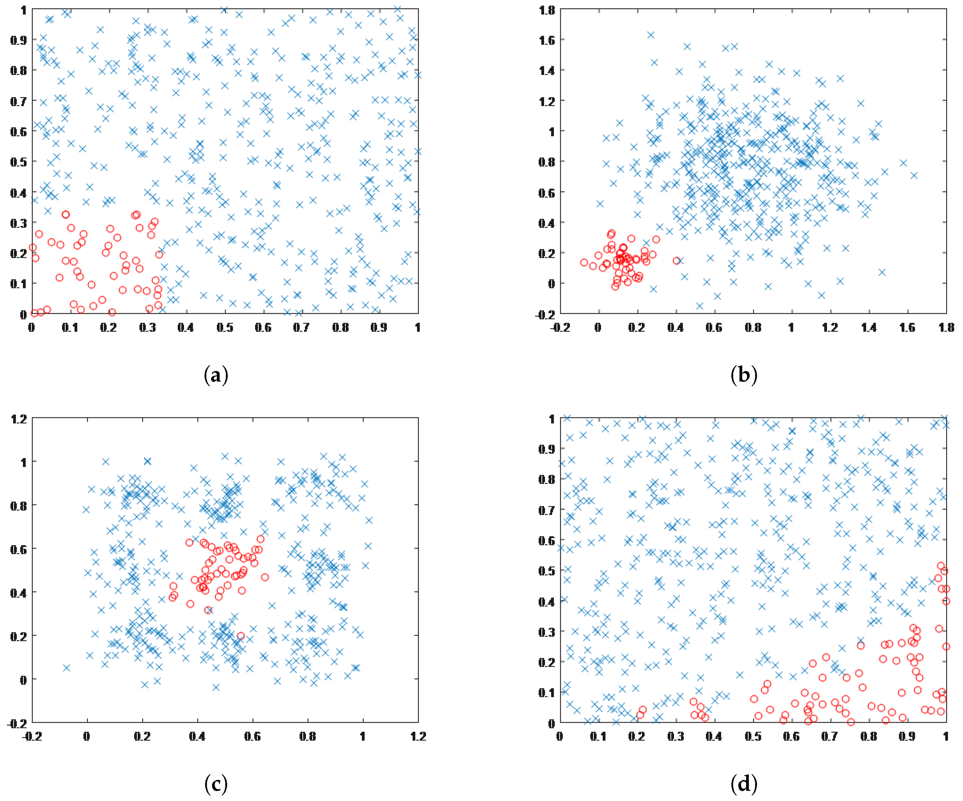
Figure 2.
Box plots illustration of the compared methods.

Table 1.
Comparison of weighted extreme learning machine (ELM) vs. NWELM on artificial data sets.
| Data Sets | Weighted ELM | NWELM | Data Sets | Weighted ELM | NWELM |
|---|---|---|---|---|---|
| Gaussian-1-1 | 0.9811 | 0.9822 | Gaussian-2-1 | 0.9629 | 0.9734 |
| Gaussian-1-2 | 0.9843 | 0.9855 | Gaussian-2-2 | 0.9551 | 0.9734 |
| Gaussian-1-3 | 0.9944 | 0.9955 | Gaussian-2-3 | 0.9670 | 0.9747 |
| Gaussian-1-4 | 0.9866 | 0.9967 | Gaussian-2-4 | 0.9494 | 0.9649 |
| Gaussian-1-5 | 0.9866 | 0.9833 | Gaussian-2-5 | 0.9467 | 0.9724 |
| Gaussian-1-6 | 0.9899 | 0.9685 | Gaussian-2-6 | 0.9563 | 0.9720 |
| Gaussian-1-7 | 0.9833 | 0.9685 | Gaussian-2-7 | 0.9512 | 0.9629 |
| Gaussian-1-8 | 0.9967 | 0.9978 | Gaussian-2-8 | 0.9644 | 0.9785 |
| Gaussian-1-9 | 0.9944 | 0.9798 | Gaussian-2-9 | 0.9441 | 0.9559 |
| Gaussian-1-10 | 0.9846 | 0.9898 | Gaussian-2-10 | 0.9402 | 0.9623 |
| Uniform-1 | 0.9836 | 0.9874 | Complex-1 | 0.9587 | 0.9481 |
| Uniform-2 | 0.9798 | 0.9750 | Complex-2 | 0.9529 | 0.9466 |
| Uniform-3 | 0.9760 | 0.9823 | Complex-3 | 0.9587 | 0.9608 |
| Uniform-4 | 0.9811 | 0.9836 | Complex-4 | 0.9482 | 0.9061 |
| Uniform-5 | 0.9811 | 0.9823 | Complex-5 | 0.9587 | 0.9297 |
| Uniform-6 | 0.9772 | 0.9772 | Complex-6 | 0.9409 | 0.9599 |
| Uniform-7 | 0.9734 | 0.9403 | Complex-7 | 0.9644 | 0.9563 |
| Uniform-8 | 0.9785 | 0.9812 | Complex-8 | 0.9575 | 0.9553 |
| Uniform-9 | 0.9836 | 0.9762 | Complex-9 | 0.9551 | 0.9446 |
| Uniform-10 | 0.9695 | 0.9734 | Complex-10 | 0.9351 | 0.9470 |
Table 2.
Real data sets and their attributes.
| Data Sets | Features (#) | Training Data (#) | Test Data (#) | Imbalance Ratio |
|---|---|---|---|---|
| yeast-1-2-8-9_vs_7 | 8 | 757 | 188 | 0.0327 |
| abalone9_18 | 8 | 584 | 147 | 0.0600 |
| glass-0-1-6_vs_2 | 9 | 153 | 39 | 0.0929 |
| vowel0 | 13 | 790 | 198 | 0.1002 |
| yeast-0-5-6-7-9_vs_4 | 8 | 422 | 106 | 0.1047 |
| page-blocks0 | 10 | 4377 | 1095 | 0.1137 |
| yeast3 | 8 | 1187 | 297 | 0.1230 |
| ecoli2 | 7 | 268 | 68 | 0.1806 |
| new-thyroid1 | 5 | 172 | 43 | 0.1944 |
| new-thyroid2 | 5 | 172 | 43 | 0.1944 |
| ecoli1 | 7 | 268 | 68 | 0.2947 |
| glass-0-1-2-3_vs_4-5-6 | 9 | 171 | 43 | 0.3053 |
| vehicle0 | 18 | 676 | 170 | 0.3075 |
| vehicle1 | 18 | 676 | 170 | 0.3439 |
| haberman | 3 | 244 | 62 | 0.3556 |
| yeast1 | 8 | 1187 | 297 | 0.4064 |
| glass0 | 9 | 173 | 43 | 0.4786 |
| iris0 | 4 | 120 | 30 | 0.5000 |
| pima | 8 | 614 | 154 | 0.5350 |
| wisconsin | 9 | 546 | 137 | 0.5380 |
| glass1 | 9 | 173 | 43 | 0.5405 |
Table 3.
Experimental results of binary data sets in terms of the . The best results on each data set are emphasized in bold-face.
Table 3.
Experimental results of binary data sets in terms of the . The best results on each data set are emphasized in bold-face.
| Data (Imbalance Ratio) | ||||||||
|---|---|---|---|---|---|---|---|---|
| Gaussian Kernel | Radial Base Kernel | |||||||
| Unweighted ELM | Weighted ELM max (, ) | SVM | Neutrosophic Weighted ELM | |||||
| C | C | C | ||||||
| imbalance ratio: 0, 0.2 | yeast-1-2-8-9_vs_7 (0.0327) | 2 | 60.97 | 71.41 | 47.88 | 77.57 | ||
| abalone9_18 (0.0600) | 72.71 | 89.76 | 51.50 | 94.53 | ||||
| glass-0-1-6_vs_2 (0.0929) | 63.20 | 83.59 | 51.26 | 91.86 | ||||
| vowel0 (0.1002) | 100.00 | 100.00 | 99.44 | 100.00 | ||||
| yeast-0-5-6-7-9_vs_4 (0.1047) | 68.68 | 82.21 | 62.32 | 85.29 | ||||
| page-blocks0 (0.1137) | 89.62 | 93.61 | 87.72 | 93.25 | ||||
| yeast3 (0.1230) | 84.13 | 93.11 | 84.71 | 93.20 | ||||
| ecoli2 (0.1806) | 94.31 | 94.43 | 92.27 | 95.16 | ||||
| new-thyroid1 (0.1944) | 99.16 | 99.72 | 96.75 | 100.00 | ||||
| new-thyroid2 (0.1944) | 99.44 | 99.72 | 98.24 | 100.00 | ||||
| imbalance ratio: 0.2, 1 | ecoli1 (0.2947) | 88.75 | 91.04 | 87.73 | 92.10 | |||
| glass-0-1-2-3_vs_4-5-6 (0.3053) | 93.26 | 95.41 | 91.84 | 95.68 | ||||
| vehicle0 (0.3075) | 99.36 | 99.36 | 96.03 | 99.36 | ||||
| vehicle1 (0.3439) | 80.60 | 86.74 | 66.04 | 88.06 | ||||
| haberman (0.3556) | 57.23 | 66.26 | 37.35 | 67.34 | ||||
| yeast1 (0.4064) | 65.45 | 73.17 | 61.05 | 73.19 | ||||
| glass0 (0.4786) | 85.35 | 85.65 | 79.10 | 85.92 | ||||
| iris0 (0.5000) | 100.00 | 100.00 | 98.97 | 100.00 | ||||
| pima (0.5350) | 71.16 | 75.58 | 70.17 | 76.35 | ||||
| wisconsin (0.5380) | 97.18 | 97.70 | 95.67 | 98.22 | ||||
| glass1 (0.5405) | 77.48 | 80.35 | 69.64 | 81.77 | ||||
Table 4.
Experimental result of binary data sets in terms of the average area under curve (AUC). The best results on each data set are emphasized in bold-face.
Table 4.
Experimental result of binary data sets in terms of the average area under curve (AUC). The best results on each data set are emphasized in bold-face.
| AUC | Data (Imbalance Ratio) | |||||||
|---|---|---|---|---|---|---|---|---|
| Gaussian Kernel | Radial Base Kernel | |||||||
| Unweighted ELM | Weighted ELM max (, ) | SVM | Neutrosophic Weighted ELM | |||||
| C | AUC (%) | C | AUC (%) | AUC (%) | C | AUC (%) | ||
| imbalance ratio: 0, 0.2 | yeast-1-2-8-9_vs_7 (0.0327) | 2 | 61.48 | 65.53 | 56.67 | 74.48 | ||
| abalone9_18 (0.0600) | 73.05 | 89.28 | 56.60 | 95.25 | ||||
| glass-0-1-6_vs_2 (0.0929) | 67.50 | 61.14 | 53.05 | 93.43 | ||||
| vowel0 (0.1002) | 93.43 | 99.22 | 99.44 | 99.94 | ||||
| yeast-0-5-6-7-9_vs_4 (0.1047) | 66.35 | 80.09 | 69.88 | 82.11 | ||||
| page-blocks0 (0.1137) | 67.42 | 71.55 | 88.38 | 91.49 | ||||
| yeast3 (0.1230) | 69.28 | 90.92 | 83.92 | 93.15 | ||||
| ecoli2 (0.1806) | 71.15 | 94.34 | 92.49 | 94.98 | ||||
| new-thyroid1 (0.1944) | 90.87 | 98.02 | 96.87 | 100.00 | ||||
| new-thyroid2 (0.1944) | 84.29 | 96.63 | 98.29 | 100.00 | ||||
| imbalance ratio: 0.2, 1 | ecoli1 (0.2947) | 66.65 | 90.28 | 88.16 | 92.18 | |||
| glass-0-1-2-3_vs_4-5-6 (0.3053) | 88.36 | 93.94 | 92.02 | 95.86 | ||||
| vehicle0 (0.3075) | 71.44 | 62.41 | 96.11 | 98.69 | ||||
| vehicle1 (0.3439) | 58.43 | 51.80 | 69.10 | 88.63 | ||||
| haberman (0.3556) | 68.11 | 55.44 | 54.05 | 72.19 | ||||
| yeast1 (0.4064) | 56.06 | 70.03 | 66.01 | 73.66 | ||||
| glass0 (0.4786) | 74.22 | 75.99 | 79.81 | 81.41 | ||||
| iris0 (0.5000) | 100.00 | 100.00 | 99.00 | 100.00 | ||||
| pima (0.5350) | 59.65 | 50.01 | 71.81 | 75.21 | ||||
| wisconsin (0.5380) | 83.87 | 80.94 | 95.68 | 98.01 | ||||
| glass1 (0.5405) | 75.25 | 80.46 | 72.32 | 81.09 | ||||
Table 5.
Paired t-test results between each method and the proposed method for AUC results.
| Data Sets | Unweighted ELM | Weighted ELM | SVM | |
|---|---|---|---|---|
| imbalance ratio: 0, 0.2 | yeast-1-2-8-9_vs_7 (0.0327) | 0.0254 | 0.0561 | 0.0018 |
| abalone9_18 (0.0600) | 0.0225 | 0.0832 | 0.0014 | |
| glass-0-1-6_vs_2 (0.0929) | 0.0119 | 0.0103 | 0.0006 | |
| vowel0 (0.1002) | 0.0010 | 0.2450 | 0.4318 | |
| yeast-0-5-6-7-9_vs_4 (0.1047) | 0.0218 | 0.5834 | 0.0568 | |
| page-blocks0 (0.1137) | 0.0000 | 0.0000 | 0.0195 | |
| yeast3 (0.1230) | 0.0008 | 0.0333 | 0.0001 | |
| ecoli2 (0.1806) | 0.0006 | 0.0839 | 0.0806 | |
| new-thyroid1 (0.1944) | 0.0326 | 0.2089 | 0.1312 | |
| new-thyroid2 (0.1944) | 0.0029 | 0.0962 | 0.2855 | |
| imbalance ratio: 0.2, 1 | ecoli1 (0.2947) | 0.0021 | 0.1962 | 0.0744 |
| glass-0-1-2-3_vs_4-5-6 (0.3053) | 0.0702 | 0.4319 | 0.0424 | |
| vehicle0 (0.3075) | 0.0000 | 0.0001 | 0.0875 | |
| vehicle1 (0.3439) | 0.0000 | 0.0000 | 0.0001 | |
| haberman (0.3556) | 0.1567 | 0.0165 | 0.0007 | |
| yeast1 (0.4064) | 0.0001 | 0.0621 | 0.0003 | |
| glass0 (0.4786) | 0.0127 | 0.1688 | 0.7072 | |
| iris0 (0.5000) | NaN | NaN | 0.3739 | |
| pima (0.5350) | 0.0058 | 0.0000 | 0.0320 | |
| wisconsin (0.5380) | 0.0000 | 0.0002 | 0.0071 | |
| glass1 (0.5405) | 0.0485 | 0.8608 | 0.0293 |
Table 6.
Friedman Aligned Ranks test (significance level of 0.05).
| Statistic | p-Value | Result | |
|---|---|---|---|
| 29.6052 | 0.0000 | H0 is rejected | |
| Ranking | |||
| Algorithm | Rank | ||
| ELM | 21.7619 | ||
| WELM | 38.9047 | ||
| SVM | 41.5238 | ||
| NWELM | 67.8095 | ||
| Comparison | Statistic | Adjusted p-Value | Result |
| NWELM vs. ELM | 6.1171 | 0.0000 | H0 is rejected |
| NWELM vs. WELM | 3.8398 | 0.0003 | H0 is rejected |
| NWELM vs. SVM | 3.4919 | 0.0005 | H0 is rejected |
Table 7.
Comparison of the proposed method with two ensemble-based weighted ELM methods.
| Vote-Based Ensemble | DE-Based Ensemble | NWELM | ||||
|---|---|---|---|---|---|---|
| C | C | C | ||||
| glass1 | 74.32 | 77.72 | 81.77 | |||
| haberman | 63.10 | 62.68 | 67.34 | |||
| ecoli1 | 89.72 | 91.39 | 92.10 | |||
| new-thyroid2 | 99.47 | 99.24 | 100.00 | |||
| yeast3 | 94.25 | 94.57 | 93.20 | |||
| ecoli3 | 88.68 | 89.50 | 92.16 | |||
| glass2 | 86.45 | 87.51 | 85.58 | |||
| yeast1_7 | 78.95 | 78.94 | 84.66 | |||
| ecoli4 | 96.33 | 96.77 | 98.85 | |||
| abalone9_18 | 89.24 | 90.13 | 94.53 | |||
| glass5 | 94.55 | 94.55 | 95.02 | |||
| yeast5 | 94.51 | 94.59 | 98.13 | |||
| Average | 87.46 | 88.13 | 90.53 | |||
© 2017 by the authors. Licensee MDPI, Basel, Switzerland. This article is an open access article distributed under the terms and conditions of the Creative Commons Attribution (CC BY) license (http://creativecommons.org/licenses/by/4.0/).
Share and Cite
MDPI and ACS Style
Akbulut, Y.; Şengür, A.; Guo, Y.; Smarandache, F. A Novel Neutrosophic Weighted Extreme Learning Machine for Imbalanced Data Set. Symmetry 2017, 9, 142. https://doi.org/10.3390/sym9080142
AMA Style
Akbulut Y, Şengür A, Guo Y, Smarandache F. A Novel Neutrosophic Weighted Extreme Learning Machine for Imbalanced Data Set. Symmetry. 2017; 9(8):142. https://doi.org/10.3390/sym9080142
Chicago/Turabian StyleAkbulut, Yaman, Abdulkadir Şengür, Yanhui Guo, and Florentin Smarandache. 2017. "A Novel Neutrosophic Weighted Extreme Learning Machine for Imbalanced Data Set" Symmetry 9, no. 8: 142. https://doi.org/10.3390/sym9080142
Note that from the first issue of 2016, this journal uses article numbers instead of page numbers. See further details here.