On Brane Solutions with Intersection Rules Related to Lie Algebras

Abstract

The review is devoted to exact solutions with hidden symmetries arising in a multidimensional gravitational model containing scalar fields and antisymmetric forms. These solutions are defined on a manifold of the form $M=M_0\times M_1\times \dots \times M_n$, where all $M_i$ with $i\ge 1$ are fixed Einstein (e.g., Ricci-flat) spaces. We consider a warped product metric on M. Here, $M_0$ is a base manifold, and all scale factors (of the warped product), scalar fields and potentials for monomial forms are functions on $M_0$. The monomial forms (of the electric or magnetic type) appear in the so-called composite brane ansatz for fields of forms. Under certain restrictions on branes, the sigma-model approach for the solutions to field equations was derived in earlier publications with V.N.Melnikov. The sigma model is defined on the manifold $M_0$ of dimension $d_0\ne 2$. By using the sigma-model approach, several classes of exact solutions, e.g., solutions with harmonic functions, S-brane, black brane and fluxbrane solutions, are obtained. For $d_0=1$, the solutions are governed by moduli functions that obey Toda-like equations. For certain brane intersections related to Lie algebras of finite rank—non-singular Kac–Moody (KM) algebras—the moduli functions are governed by Toda equations corresponding to these algebras. For finite-dimensional semi-simple Lie algebras, the Toda equations are integrable, and for black brane and fluxbrane configurations, they give rise to polynomial moduli functions. Some examples of solutions, e.g., corresponding to finite dimensional semi-simple Lie algebras, hyperbolic KM algebras: $H_2(q,q)$, $A{E}_3$, $H{A}_2^{(1)}$, $E_{10}$ and Lorentzian KM algebra $P_{10}$, are presented.

1. Introduction

In this review, we deal with certain aspects of multidimensional models of gravity, which are rather popular at present time. As is widely known, the history of the multidimensional approach begins with the well-known papers of Kaluza and Klein on five-dimensional theories, which were continued then by Jordan in his works. These papers were in some sense a source of inspiration for Brans and Dicke in their well-known work on a scalar-tensor gravitational theory. After their work, many investigations were performed in models with fundamental scalar fields, both conformal and non-conformal; see [1] and the references therein.

A revival of the ideas of many dimensions started in the 1970s and continues now, mainly due to the development of unified theories. In the 1970s, interest in multidimensional gravitational models was stimulated mainly by: (i) the ideas of gauge theories leading to a non-Abelian generalization of the Kaluza–Klein approach and (ii) by supergravitational theories [2,3].

In the 1980s, the supergravitational theories “gave the baton” to the superstring theory [4] and in the 1990s to the so-called M-theory [5,6].

Usually, having a multidimensional model, one can obtain a four-dimensional one by a dimensional reduction based on the decomposition of the manifold:

$$M=M^4\times M_{\mathrm{int}},$$

(1)

where $M^4$ is a four-dimensional manifold and $M_{\mathrm{int}}$ is some internal manifold (widely considered to be compact).

Here, we overview a sigma-model approach and several classes of exact solutions for the multidimensional gravitational model governed by the Lagrangian:

$$\mathcal{L}=R[g]-2\mathsf{\Lambda }-h_{\alpha \beta }{g}^{MN}{\partial }_M{\phi }^{\alpha }{\partial }_N{\phi }^{\beta }-\sum _a\frac{1}{n_a!}exp(2{\lambda }_{a\alpha }{\phi }^{\alpha }){(F^a)}^2,$$

(2)

where g is metric, $F^a=d{A}^a$ are forms (of ranks $n_a$), ${\phi }^{\alpha }$ are scalar fields, ${\lambda }_a=({\lambda }_{a\alpha })$ are certain vectors and $\mathsf{\Lambda }$ is a cosmological constant (the matrix $(h_{\alpha \beta })$ is invertible). The Lagrangians of such a type may describe (pure bosonic) solutions in supergravitational models [7], when the so-called Chern–Simons terms are zero.

We deal with the solutions having a block-diagonal (warped-product) metrics g defined on the D-dimensional product manifold M, i.e.,

$$g=e^{2\gamma }{g}^0+\sum _{i=1}^n{e}^{2{\varphi }^i}{g}^i,M=M_0\times M_1\times \dots \times M_n,$$

(3)

where $g^0$ is a metric on $M_0$ and $g^i$ are fixed Einstein (or Ricci-flat) metrics on $M_i$, $i>0$. The moduli $\gamma ,{\varphi }^i$ and scalar fields ${\phi }^{\alpha }$ are functions on $M_0$, and fields of forms are also governed by several scalar functions on $M_0$. Any $F^a$ is supposed to be a sum of (linear independent) monoms, corresponding to electric or magnetic p-branes (p-dimensional analogues of membranes), i.e., the so-called composite p-brane ansatz is considered.

Here, we are interested in brane solutions, which have intersection rules related to a certain subclass of Lie algebras, namely non-singular Kac–Moody (KM) algebras. Kac–Moody (KM) Lie algebras [8,9,10] play a rather important role in different areas of mathematical physics (see [10,11,12,13] and the references therein).

We recall that KM Lie algebra is a Lie algebra generated by the relations [10]:

$$\begin{array}{c}\hfill [h_i,h_j]=0,[e_i,f_j]={\delta }_{ij}{h}_j,\end{array}$$

(4)

$$\begin{array}{c}\hfill [h_i,e_j]=A_{ij}{e}_j,[h_i,f_j]=-A_{ij}{f}_j,\end{array}$$

(5)

$$\begin{array}{c}\hfill {(\mathrm{ad}{e}_i)}^{1-A_{ij}}(e_j)=0(i\ne j),\end{array}$$

(6)

$$\begin{array}{c}\hfill {(\mathrm{ad}{f}_i)}^{1-A_{ij}}(f_j)=0(i\ne j).\end{array}$$

(7)

Here, $A=(A_{ij})$ is a generalized Cartan matrix, $i,j=1,\dots ,r$, and r is the rank of the KM algebra. This means that all $A_{ii}=2$; $A_{ij}$ for $i\ne j$ are non-positive integers, and $A_{ij}=0$ implies $A_{ji}=0$.

In what follows, the matrix A is restricted to be non-degenerate (i.e., $detA\ne 0$) and symmetrizable i.e., $A=B\mathcal{D}$, where B is a symmetric matrix and $\mathcal{D}$ is an invertible diagonal matrix ($\mathcal{D}$ may be chosen in such way that all of its entries ${\mathcal{D}}_{ii}$ are positive rational numbers [10]). Here, we do not consider singular KM algebras with $detA=0$, e.g., affine ones. Recall that affine KM algebras are of much interest for conformal field theories, superstring theories, etc. [4,11].

In the case when A is positive definite (the Euclidean case), we get ordinary finite dimensional Lie algebras [10,11]. For non-Euclidean signatures of A, all KM algebras are infinite-dimensional. Among these, the Lorentzian KM algebras with pseudo-Euclidean signatures $(-,+,\dots ,+)$ for the Cartan matrix A are of current interest, since they contain a subclass of the so-called hyperbolic KM algebras widely used in modern mathematical physics. Hyperbolic KM algebras are by definition Lorentzian Kac–Moody algebras with the property that removing any node from their Dynkin diagram leaves one with a Dynkin diagram of the affine or finite type. The hyperbolic KM algebras can be completely classified [14,15,16] and have rank $2\le r\le 10$. For $r\ge 3$, there is a finite number of hyperbolic algebras. For rank 10, there are four algebras, known as $E_{10}$, $B{E}_{10}$, $C{E}_{10}$ and $D{E}_{10}$. Hyperbolic KM algebras appeared in ordinary gravity [17] (${\mathcal{F}}_3=A{E}_3=H_3$), supergravity: [18,19] ($E_{10}$), [20] (${\mathcal{F}}_3$), strings [21], etc.

The growth of interest in hyperbolic algebras in theoretical and mathematical physics appeared in 2001 after the publication of Damour and Henneaux [22] devoted to a description of chaotic (BKL-type [23]) behavior near the singularity in string-inspired low energy models (e.g., supergravitational ones) [24] (see also [25]). It should be noted that these results were based on a billiard approach in multidimensional cosmology with different matter sources (for $D=4$ suggested by Chitre [26]) elaborated in our papers [27,28,29,30,31] (see also [32,33,34]).

The description of oscillating behavior near the singularity in $D=11$ supergravity [2] (which is related to M-theory [5,6]) in terms of motion of a point-like particle in a nine-dimensional billiard (of finite volume) corresponding to the Weyl chamber of the hyperbolic KM algebra $E_{10}$ inspired another description of $D=11$ supergravity in [35]: a formal “small tension” expansion of $D=11$ supergravity near a space-like singularity was shown to be equivalent (at least up to 30th order in height) to a null geodesic motion in the infinite dimensional coset space ${\mathcal{E}}_{10}/K({\mathcal{E}}_{10})$ (here, $K({\mathcal{E}}_{10})$ is the maximal compact subgroup of the hyperbolic Kac–Moody group ${\mathcal{E}}_{10}(R)$).

Recall that $E_{10}$ KM algebra is an over-extension of the finite dimensional Lie algebra $E_8$, i.e., $E_{10}=E_8^{++}$. However, there is another extension of $E_8$—the so-called very extended Kac–Moody algebra of the $E_8$ algebra—called $E_{11}=E_8^{+++}$ (to get an understanding of very extended algebras and some of their properties, see [36] and the references therein). It has been proposed by P.West that the Lorentzian (non-hyperbolic) KM algebra $E_{11}$ is responsible for a hidden algebraic structure characterizing 11-dimensional supergravity [37]. The same very extended algebra occurs in $IIA$ [37] and $IIB$ supergravities [38]. Moreover, it was conjectured that an analogous hidden structure is realized in the effective action of the bosonic string (with the KM algebra $k_{27}=D_{24}^{+++}$) [37] and also for pure D dimensional gravity (with the KM algebra $A_{D-3}^{+++}$ [39]). It has been suggested in [40] that all of the so-called maximally-oxidized theories (see also [13]) possess the very extension $G^{+++}$ of the simple Lie algebra G. It was shown in [41] that the BPSsolutions of the oxidized theory of a simply laced group $\mathcal{G}$ form representations of a subgroup of the Weyl transformations of the algebra $G^{+++}$. For other aspects of very-extended Kac–Moody algebras (e.g., $E_{11}$), see also [42,43,44,45] and the references therein.

In this paper, we briefly review another possibility for utilizing non-singular (e.g., hyperbolic) KM algebras suggested in three of our papers [46,47,48]. This possibility (implicitly assumed also in [49,50,51,52,53,54]) is related to certain classes of exact solutions describing intersecting composite branes in a multidimensional gravitational model containing scalar fields and antisymmetric forms defined on (warped) product manifolds $M=M_0\times M_1\times \dots \times M_n$, where $M_i$ are Ricci-flat spaces ($i\ge 1$). From a pure mathematical point of view, these solutions may be obtained from sigma-models or Toda chains corresponding to certain non-singular KM algebras. The information about the (hidden) KM algebra is encoded in intersection rules, which relate the dimensions of brane intersections with non-diagonal components of the generalized Cartan matrix A [55]. We deal here with generalized Cartan matrices of the form:

$$A_{s{s}^{\prime }}\equiv \frac{2(U^s,U^{s^{\prime }})}{(U^{s^{\prime }},U^{s^{\prime }})},$$

(8)

$s,s^{\prime }\in S$, with $(U^s,U^s)\ne 0$, for all $s\in S$ (S is a finite set). Here, $U^s$ are the so-called brane (co-)vectors. They are linear functions on ${\mathbb{R}}^N$, where $N=n+l$, and l is the number of scalar fields. The indefinite scalar product $(.,.)$ [56] is defined on ${({\mathbb{R}}^N)}^{*}$ and has the signature $(-1,+1,\dots ,+1)$ when all scalar fields have positive kinetic terms, i.e., there are no phantoms (or ghosts). The matrix A is symmetrizable. U^s-vectors may be put in one-to-one correspondence with simple roots ${\alpha }_s$ of the generalized KM algebra after a suitable normalizing. For indecomposable A (when the KM algebra is simple), the matrices $((U^s,U^{s^{\prime }}))$ and $(({\alpha }_s|{\alpha }_{s^{\prime }}))$ are proportional to each other. Here, $(.|.)$ is a non-degenerate bilinear symmetric form on a root space obeying $({\alpha }_s|{\alpha }_s)>0$ for all simple roots ${\alpha }_s$ [10].

We note that the minisuperspace bilinear form $(.,.)$ coming from the multidimensional gravitational model [56] should not coincide with the bilinear form $(.|.)$ from [10], and hence, there exist physical examples where all $(U^s,U^s)$ are negative. Some examples of this are given below (see Section 5). For $D=11$ supergravity and ten-dimensional $IIA$, $IIB$ supergravities, all $(U^s,U^s)=2$ [44,55] and corresponding KM algebras are simply laced. It was shown in our papers [29,30,31] that the inequality $(U^s,U^s)>0$ is a necessary condition for the formation of the billiard wall (ifone approaches the singularity) by the s-th matter source (e.g., a fluid component or a brane).

The scalar products for brane vectors $U^s$ were found in [56] (for the electric case, see also [57,58,59]):

$$(U^s,U^{s^{\prime }})=d_{s{s}^{\prime }}+\frac{d_s{d}_{s^{\prime }}}{2-D}+{\chi }_s{\chi }_{s^{\prime }}<{\lambda }_s,{\lambda }_{s^{\prime }}>,$$

(9)

where $d_s$ and $d_{s^{\prime }}$ are dimensions of the brane world volumes corresponding to branes s and $s^{\prime }$, respectively, $d_{s{s}^{\prime }}$ is the dimension of intersection of the brane world volumes, D is the total space-time dimension, ${\chi }_s=+1,-1$ for electric or magnetic brane, respectively, and $<{\lambda }_s,{\lambda }_{s^{\prime }}>$ is the non-degenerate scalar product of the l-dimensional dilatonic coupling vectors ${\lambda }_s$ and ${\lambda }_{s^{\prime }}$ corresponding to branes s and $s^{\prime }$.

Relations (2) and (9) define the brane intersection rules [55]:

$$\begin{array}{c}\hfill d_{s{s}^{\prime }}=d_{s{s}^{\prime }}^o+\frac{1}{2}{K}_{s^{\prime }}{A}_{s{s}^{\prime }},\end{array}$$

(10)

$s\ne s^{\prime }$, where $K_s=(U^s,U^s)$ and:

$$d_{s{s}^{\prime }}^o=\frac{d_s{d}_{s^{\prime }}}{D-2}-{\chi }_s{\chi }_{s^{\prime }}<{\lambda }_s,{\lambda }_{s^{\prime }}>$$

(11)

are the dimensions of the so-called orthogonal (or $A_1\oplus \dots \oplus A_1$-) intersections of branes following from the orthogonality conditions [56]:

$$(U^s,U^{s^{\prime }})=0,$$

(12)

$s\ne s^{\prime }$. The orthogonality relations (12) for brane intersections in the non-composite electric case were suggested in [57,58] and for the composite electric case in [59].

Relations (9) and (11) were derived in [56] for rather general assumptions: the branes were composite; the number of scalar fields l was arbitrary; as well as the signature of the bilinear form $<.,.>$ (or equivalently, the signature of the kinetic term for scalar fields), Ricci-flat factor spaces $M_i$ had arbitrary dimensions $d_i$ and signatures. The intersection rules (11) appeared earlier (in different notations) in [60,61,62] when all $d_i=1$ ($i>0$), and $<.,.>$ was positive definite (in [60,61], $l=1$, and total space-time had a pseudo-Euclidean signature). The intersection rules (11) were also used in [55,63,64,65] in the context of intersecting black brane solutions.

It was proven in [66] that the target space of the sigma model describing composite electro-magnetic brane configurations on the product of several Ricci-flat spaces is a homogeneous (coset) space $G/H$. It is locally symmetric (i.e., the Riemann tensor is covariantly constant: $\mathsf{\nabla }Riem=0$) if and only if:

$$(U^s-U^{s^{\prime }})(U^s,U^{s^{\prime }})=0$$

(13)

for all s and $s^{\prime }$, i.e., when any two brane vectors $U^s$ and $U^{s^{\prime }}$, $s\ne s^{\prime }$, are either coinciding $U^s=U^{s^{\prime }}$ or orthogonal $(U^s,U^{s^{\prime }})=0$ (for two electric branes and $l=1$, see also [67]).

Now, relations for brane vectors $U^s$ (2) and (9) (with $U^s$ being identified with roots ${\alpha }_s$) are widely used in the $G^{+++}$-approach [13,41]. The orthogonality condition (12) describing the intersection of branes [56,57,58,59] was rediscovered in [44] (for some particular intersecting configurations of M-theory, it was done in [68]). It was found in the context of $G^{+++}$-algebras that the intersection rules for extremal branes are encoded in orthogonality conditions between the various roots from which the branes arise, i.e., $({\alpha }_s|{\alpha }_{s^{\prime }})=0$, $s\ne s^{\prime }$, where ${\alpha }_s$ should be real positive roots (“real” means that $({\alpha }_s|{\alpha }_s)>0$). In [44], another condition on brane, root vectors was found: ${\alpha }_s+{\alpha }_{s^{\prime }}$ should not be a root, $s\ne s^{\prime }$. The last condition is trivial for M-theory and for $IIA$ and $IIB$ supergravities, but for low energy effective actions of heterotic strings, it forbids certain intersections that do not take place due to non-zero contributions of Chern-Simons terms.

It should be noted that the orthogonality relations for brane intersections (12) appeared in 1996–1997. The standard intersection rules (11) gave back the well-known zero binding energy configurations preserving some supersymmetries. These brane configurations were originally derived from supersymmetry and duality arguments (see for example [69,70,71] and the reference therein) or by using a no-force condition (suggested for M-branes in [72]).

2. The Model

2.1. The Action

We consider the model governed by action:

$$\begin{array}{cc}\hfill S=& \frac{1}{2{\kappa }^2}{\int }_M{d}^{D}z\sqrt{\left|g\right|}\{R[g]-2\mathsf{\Lambda }-h_{\alpha \beta }{g}^{MN}{\partial }_M{\phi }^{\alpha }{\partial }_N{\phi }^{\beta }\hfill \\ & -\sum _{a\in \Delta }\frac{{\theta }_a}{n_a!}exp[2{\lambda }_a(\phi )]{(F^a)}_g^2\}+S_{GH},\hfill \end{array}$$

(14)

where $g=g_{MN}d{z}^M\otimes d{z}^N$ is the metric on the manifold M, $dimM=D$, $\phi =({\phi }^{\alpha })\in {\mathbb{R}}^l$ is a vector of dilatonic scalar fields, $(h_{\alpha \beta })$ is a non-degenerate symmetric $l\times l$ matrix ($l\in \mathbb{N}$), ${\theta }_a\ne 0$,

$$F^a=d{A}^a=\frac{1}{n_a!}{F}_{M_1\dots M_{n_a}}^{a}d{z}^{M_1}\wedge \dots \wedge d{z}^{M_{n_a}}$$

is an $n_a$-form ($n_a\ge 2$) on a D-dimensional manifold M, $\mathsf{\Lambda }$ is a cosmological constant and ${\lambda }_a$ is a one-form on ${\mathbb{R}}^l$: ${\lambda }_a(\phi )={\lambda }_{a\alpha }{\phi }^{\alpha }$, $a\in \Delta$, $\alpha =1,\dots ,l$. In (14), we denote $\left|g\right|=|det(g_{MN})|$, ${(F^a)}_g^2=F_{M_1\dots M_{n_a}}^a{F}_{N_1\dots N_{n_a}}^a{g}^{M_1{N}_1}\dots g^{M_{n_a}{N}_{n_a}},$ $a\in \Delta$, where $\Delta$ is some finite set (for example, of positive integers), and $S_{\mathrm{GH}}$ is the standard Gibbons–Hawking boundary term [73]. In models with one time, all ${\theta }_a=1$ when the signature of the metric is $(-1,+1,\dots ,+1)$. ${\kappa }^2$ is the multidimensional gravitational constant.

2.2. Ansatz for Composite Branes

Let us consider the manifold:

$$M=M_0\times M_1\times \dots \times M_n,$$

(15)

with the metric:

$$g=e^{2\gamma (x)}{\widehat{g}}^0+\sum _{i=1}^n{e}^{2{\varphi }^i(x)}{\widehat{g}}^i,$$

(16)

where $g^0=g_{\mu \nu }^0(x)d{x}^{\mu }\otimes d{x}^{\nu }$ is an arbitrary metric with any signature on the manifold $M_0$ and $g^i=g_{m_i{n}_i}^i(y_i)d{y}_i^{m_i}\otimes d{y}_i^{n_i}$ is a metric on $M_i$ satisfying the equation:

$$R_{m_i{n}_i}[g^i]={\xi }_i{g}_{m_i{n}_i}^i,$$

(17)

$m_i,n_i=1,\dots ,d_i$; ${\xi }_i=\mathrm{const}$, $i=1,\dots ,n$. Here, ${\widehat{g}}^i=p_i^{*}{g}^i$ is the pullback of the metric $g^i$ to the manifold M by the canonical projection: $p_i:M\to M_i$, $i=0,\dots ,n$. Thus, $(M_i,g^i)$ are Einstein spaces, $i=1,\dots ,n$. The functions $\gamma ,{\varphi }^i:M_0\to \mathbb{R}$ are smooth. We denote $d_{\nu }=\dim M_{\nu }$; $\nu =0,\dots ,n$; $D={\sum }_{\nu =0}^n{d}_{\nu }$. We put any manifold $M_{\nu }$, $\nu =0,\dots ,n$, to be oriented and connected. Then, the volume $d_i$-form:

$${\tau }_i\equiv \sqrt{|g^i(y_i)|}d{y}_i^1\wedge \dots \wedge d{y}_i^{d_i},$$

(18)

and signature parameter:

$$\epsilon (i)\equiv \mathrm{sign}(det(g_{m_i{n}_i}^i))=\pm 1$$

(19)

are correctly defined for all $i=1,\dots ,n$.

Let $\mathsf{\Omega }=\mathsf{\Omega }(n)$ be a set of all non-empty subsets of $\{1,\dots ,n\}$. The number of elements in $\mathsf{\Omega }$ is $\left|\mathsf{\Omega }\right|=2^n-1$. For any $I=\{i_1,\dots ,i_k\}\in \mathsf{\Omega }$, $i_1<\dots <i_k$, we denote:

$$\begin{array}{c}\hfill \tau (I)\equiv {\widehat{\tau }}_{i_1}\wedge \dots \wedge {\widehat{\tau }}_{i_k},\end{array}$$

(20)

$$\begin{array}{c}\hfill \epsilon (I)\equiv \epsilon (i_1)\dots \epsilon (i_k),\end{array}$$

(21)

$$\begin{array}{c}\hfill M_I\equiv M_{i_1}\times \dots \times M_{i_k},\end{array}$$

(22)

$$\begin{array}{c}\hfill d(I)\equiv \sum _{i\in I}{d}_i.\end{array}$$

(23)

Here, ${\widehat{\tau }}_i=p_i^{*}{\widehat{\tau }}_i$ is the pullback of the form ${\tau }_i$ to the manifold M by the canonical projection: $p_i:M\to M_i$, $i=1,\dots ,n$. We also put $\tau (\varnothing )=\epsilon (\varnothing )=1$ and $d(\varnothing )=0$.

For fields of forms, we consider the following composite electromagnetic ansatz:

$$\begin{array}{c}\hfill F^a=\sum _{I\in {\mathsf{\Omega }}_{a,e}}{\mathcal{F}}^{(a,e,I)}+\sum _{J\in {\mathsf{\Omega }}_{a,m}}{\mathcal{F}}^{(a,m,J)}\end{array}$$

(24)

where:

$$\begin{array}{c}\hfill {\mathcal{F}}^{(a,e,I)}=d{\mathsf{\Phi }}^{(a,e,I)}\wedge \tau (I),\end{array}$$

(25)

$$\begin{array}{c}\hfill {\mathcal{F}}^{(a,m,J)}=e^{-2{\lambda }_a(\phi )}*>(d{\mathsf{\Phi }}^{(a,m,J)}\wedge \tau (J))\end{array}$$

(26)

are elementary forms of electric and magnetic types, respectively, $a\in \Delta$, $I\in {\mathsf{\Omega }}_{a,e}$, $J\in {\mathsf{\Omega }}_{a,m}$ and ${\mathsf{\Omega }}_{a,v}\subset \mathsf{\Omega }$, $v=e,m$. In (26), $*=*[g]$ is the Hodge operator on $(M,g)$:

$${(*\omega )}_{M_1\dots M_{D-k}}=\frac{{\left|g\right|}^{1/2}}{k!}{\epsilon }_{M_1\dots M_{D-k}{N}_1\dots N_k}{\omega }^{N_1\dots N_k},$$

where $\mathrm{rank}\omega =k$.

For scalar functions, we put:

$$\begin{array}{c}\hfill {\phi }^{\alpha }={\phi }^{\alpha }(x),{\mathsf{\Phi }}^s={\mathsf{\Phi }}^s(x),\end{array}$$

(27)

$s\in S$. Thus, ${\phi }^{\alpha }$ and ${\mathsf{\Phi }}^s$ are functions on $M_0$.

Here and below:

$$\begin{array}{c}\hfill S=S_e\bigsqcup S_m,S_v={\bigsqcup }_{a\in \Delta }\{a\}\times \{v\}\times {\mathsf{\Omega }}_{a,v},\end{array}$$

(28)

$v=e,m$. Here and in what follows, ⊔ means the union of non-intersecting sets. The set S consists of elements $s=(a_s,v_s,I_s)$, where $a_s\in \Delta$ is the color index, $v_s=e,m$ is the electro-magnetic index and set $I_s\in {\mathsf{\Omega }}_{a_s,v_s}$ describes the location of brane.

Due to (25) and (26):

$$\begin{array}{c}\hfill d(I)=n_a-1,d(J)=D-n_a-1,\end{array}$$

(29)

for $I\in {\mathsf{\Omega }}_{a,e}$ and $J\in {\mathsf{\Omega }}_{a,m}$ (i.e., in the electric and magnetic case, respectively).

2.3. The Sigma Model

Let $d_0\ne 2$ and:

$$\begin{array}{c}\hfill \gamma ={\gamma }_0(\varphi )\equiv \frac{1}{2-d_0}\sum _{j=1}^n{d}_j{\varphi }^j,\end{array}$$

(30)

i.e., the generalized harmonic gauge (frame) is used.

Here, we put two restrictions on sets of branes that guarantee the block-diagonal form of the energy-momentum tensor and the existence of the sigma-model representation (without additional constraints):

$$(\mathbf{R}\mathbf{1})d(I\cap J)\le d(I)-2,$$

(31)

for any $I,J\in {\mathsf{\Omega }}_{a,v}$, $a\in \Delta$, $v=e,m$ (here $d(I)=d(J)$) and

$$(\mathbf{R}\mathbf{2})d(I\cap J)\ne 0for{d}_0=1,d(I\cap J)\ne 1for{d}_0=3.$$

(32)

It was proven in [56] that equations of motion for the model (14) and the Bianchi identities:

$$\begin{array}{c}\hfill d{\mathcal{F}}^s=0,\end{array}$$

(33)

$s\in S_m$, for fields from (16), (24)–(27), when Restrictions (31) and (32) are imposed, are equivalent to the equations of motion for the $\sigma$-model governed by the action:

$$\begin{array}{cc}\hfill S_{\sigma 0}=& \frac{1}{2{\kappa }_0^2}\int d^{d_0}x\sqrt{|g^0|}\{R[g^0]-{\widehat{G}}_{AB}{g}^{0\mu \nu }{\partial }_{\mu }{\sigma }^A{\partial }_{\nu }{\sigma }^B\hfill \\ & -\sum _{s\in S}{\epsilon }_{s}exp(-2U_A^s{\sigma }^A)g^{0\mu \nu }{\partial }_{\mu }{\mathsf{\Phi }}^s{\partial }_{\nu }{\mathsf{\Phi }}^s-2V\},\hfill \end{array}$$

(34)

where $({\sigma }^A)=({\varphi }^i,{\phi }^{\alpha })$, $k_0\ne 0$, the index set S is defined in (28),

$$V=V(\varphi )=\mathsf{\Lambda }{e}^{2{\gamma }_0(\varphi )}-\frac{1}{2}\sum _{i=1}^n{\xi }_i{d}_i{e}^{-2{\varphi }^i+2{\gamma }_0(\varphi )}$$

(35)

is the potential,

$$\begin{array}{c}\hfill ({\widehat{G}}_{AB})=\left(\begin{array}{cc}{G}_{ij}& 0\\ 0& h_{\alpha \beta }\end{array}\right)\end{array}$$

(36)

is the target space metric with:

$$\begin{array}{c}\hfill G_{ij}=d_i{\delta }_{ij}+\frac{d_i{d}_j}{d_0-2}\end{array}$$

(37)

and co-vectors:

$$\begin{array}{c}\hfill U_A^s=U_A^s{\sigma }^A=\sum _{i\in I_s}{d}_i{\varphi }^i-{\chi }_s{\lambda }_{a_s}(\phi ),(U_A^s)=(d_i{\delta }_{i{I}_s},-{\chi }_s{\lambda }_{a_s\alpha }),\end{array}$$

(38)

$s=(a_s,v_s,I_s)$. Here, ${\chi }_e=+1$ and ${\chi }_m=-1$;

$$\begin{array}{c}\hfill {\delta }_{iI}=\sum _{j\in I}{\delta }_{ij}\end{array}$$

(39)

is an indicator of i belonging to I: ${\delta }_{iI}=1$ for $i\in I$ and ${\delta }_{iI}=0$ otherwise; and:

$$\begin{array}{c}\hfill {\epsilon }_s={(-\epsilon [g])}^{(1-{\chi }_s)/2}\epsilon (I_s){\theta }_{a_s},\end{array}$$

(40)

$s\in S$, $\epsilon [g]\equiv \mathrm{sign}det(g_{MN})$. More explicitly, (40) reads:

$${\epsilon }_s=\epsilon (I_s){\theta }_{a_s}\mathrm{for}{v}_s=e;{\epsilon }_s=-\epsilon [g]\epsilon (I_s){\theta }_{a_s},\mathrm{for}{v}_s=m.$$

(41)

For finite internal space volumes $V_i$ (e.g., compact $M_i$) and electric p-branes (i.e., all ${\mathsf{\Omega }}_{a,m}=\varnothing$), the action (34) coincides with the action (14) when ${\kappa }^2={\kappa }_0^2{\prod }_{i=1}^n{V}_i$.

3. Solutions Governed by Harmonic Functions

3.1. Solutions with a Block-Orthogonal of $U^s$ and Ricci-Flat Factor-Spaces

Here, we consider a special class of solutions to equations of motion governed by several harmonic functions when all factor spaces are Ricci-flat and the cosmological constant is zero, i.e., ${\xi }_i=\mathsf{\Lambda }=0$, $i=1,\dots ,n$. In certain situations, these solutions describe extremal black branes charged by fields of forms.

The solutions crucially depend on scalar products of U^s-vectors $(U^s,U^{s^{\prime }})$; $s,s^{\prime }\in S$, where:

$$\begin{array}{c}\hfill (U,U^{\prime })={\widehat{G}}^{AB}{U}_A{U}_B^{\prime },\end{array}$$

(42)

for $U=(U_A),U^{\prime }=(U_A^{\prime })\in {\mathbb{R}}^N$, $N=n+l$ and:

$$({\widehat{G}}^{AB})=\left(\begin{array}{cc}{G}^{ij}& 0\\ 0& h^{\alpha \beta }\end{array}\right)$$

(43)

is the inverse matrix to the matrix (36). Here, as in [74], we have:

$$G^{ij}=\frac{{\delta }^{ij}}{d_i}+\frac{1}{2-D},$$

(44)

$i,j=1,\cdots ,n$.

The scalar products (42) for vectors $U^s$ were calculated in [56] and are given by:

$$\begin{array}{c}\hfill (U^s,U^{s^{\prime }})=d(I_s\cap I_{s^{\prime }})+\frac{d(I_s)d(I_{s^{\prime }})}{2-D}+{\chi }_s{\chi }_{s^{\prime }}{\lambda }_{a_s\alpha }{\lambda }_{a_{s^{\prime }}\beta }{h}^{\alpha \beta },\end{array}$$

(45)

where $(h^{\alpha \beta })={(h_{\alpha \beta })}^{-1}$, and $s=(a_s,v_s,I_s)$, $s^{\prime }=(a_{s^{\prime }},v_{s^{\prime }},I_{s^{\prime }})$ belong to the index set S defined in (28). This relation is a very important one since it encodes brane data (e.g., intersections) via the scalar products of U-vectors.

Let:

$$S=S_1\bigsqcup \cdots \bigsqcup S_k,$$

(46)

$S_i\ne \varnothing$, $i=1,\cdots ,k$, and:

$$(U^s,U^{s^{\prime }})=0$$

(47)

for all $s\in S_i$, $s^{\prime }\in S_j$, $i\ne j$; $i,j=1,\cdots ,k$. Relation (46) means that the set S is a union of k non-intersecting (non-empty) subsets $S_1,\cdots ,S_k$. According to (47), the set of vectors $(U^s,s\in S)$ has a block-orthogonal structure with respect to the scalar product (42), i.e., it splits into k mutually orthogonal blocks $(U^s,s\in S_i)$, $i=1,\cdots ,k$.

Here, we consider exact solutions in the model (14), when vectors $(U^s,s\in S)$ obey the block-orthogonal decomposition (46) and (47) with scalar products defined in (45) [46]. These solutions were obtained from the corresponding solutions to the $\sigma$-model equations of motion [46].

Proposition 1.

Let $(M_0,g^0)$ be Ricci-flat: $R_{\mu \nu }[g^0]=0$. Then, the field configuration:

$$\begin{array}{c}\hfill g^0,{\sigma }^A=\sum _{s\in S}{\epsilon }_s{U}^{sA}{\nu }_s^{2}ln{H}_s,{\mathsf{\Phi }}^s=\frac{{\nu }_s}{H_s},\end{array}$$

(48)

$s\in S$, satisfies the field equations corresponding to the action (34) with $V=0$ if the real numbers ${\nu }_s$ obey the relations:

$$\begin{array}{c}\hfill \sum _{s^{\prime }\in S}(U^s,U^{s^{\prime }}){\epsilon }_{s^{\prime }}{\nu }_{s^{\prime }}^2=-1\end{array}$$

(49)

$s\in S$, the functions $H_s>0$ are harmonic, i.e., $\Delta [g^0]H_s=0$, $s\in S$, and $H_s$ are coinciding inside blocks: $H_s=H_{s^{\prime }}$ for $s,s^{\prime }\in S_i$, $i=1,\cdots ,k$.

Using the sigma-model solution from Proposition 1 and the relations for contra-variant components [56]:

$$\begin{array}{c}\hfill U^{si}={\delta }_{i{I}_s}-\frac{d(I_s)}{D-2},U^{s\alpha }=-{\chi }_s{\lambda }_{a_s}^{\alpha },\end{array}$$

(50)

$s=(a_s,v_s,I_s)$, we get [46]:

$$\begin{array}{c}\hfill g={\left(\prod _{s\in S}{H}_s^{2d(I_s){\epsilon }_s{\nu }_s^2}\right)}^{1/(2-D)}\left\{{\widehat{g}}^0+\sum _{i=1}^n\left(\prod _{s\in S}{H}_s^{2{\epsilon }_s{\nu }_s^2{\delta }_{i{I}_s}}\right){\widehat{g}}^i\right\},\end{array}$$

(51)

$$\begin{array}{c}\hfill {\phi }^{\alpha }=-\sum _{s\in S}{\lambda }_{a_s}^{\alpha }{\chi }_s{\epsilon }_s{\nu }_s^{2}ln{H}_s,\end{array}$$

(52)

$$\begin{array}{c}\hfill F^a=\sum _{s\in S}{\mathcal{F}}^s{\delta }_{a_s}^a,\end{array}$$

(53)

where $i=1,\cdots ,n$, $\alpha =1,\cdots ,l$, $a\in \Delta$ and:

$$\begin{array}{c}\hfill {\mathcal{F}}^s={\nu }_{s}d{H}_s^{-1}\wedge \tau (I_s),\mathrm{for}{v}_s=e,\end{array}$$

(54)

$$\begin{array}{c}\hfill {\mathcal{F}}^s={\nu }_s({*}_{0}d{H}_s)\wedge \tau ({\overline{I}}_s),\mathrm{for}{v}_s=m,\end{array}$$

(55)

$H_s$ are harmonic functions on $(M_0,g^0)$, which coincide inside blocks (i.e., $H_s=H_{s^{\prime }}$ for $s,s^{\prime }\in S_i$, $i=1,\cdots ,k$), and the relations (49) on the parameters ${\nu }_s$ are imposed. Here, the matrix $((U^s,U^{s^{\prime }}))$ and parameters ${\epsilon }_s$, $s\in S$, are defined in (45) and (40), respectively; ${\lambda }_a^{\alpha }=h^{\alpha \beta }{\lambda }_{a\beta }$, ${*}_0=*[g^0]$ is the Hodge operator on $(M_0,g^0)$, and:

$$\begin{array}{c}\hfill \overline{I}=\{1,\cdots ,n\}\backslash I\end{array}$$

(56)

is the dual set (in (55), we redefined the sign of the ${\nu }_s$-parameter).

3.2. Solutions Related to Non-Singular KM Algebras

Now, we study the solutions (51)–(55) in more detail and show that some of them may be related to non-singular KM algebras. We put:

$$\begin{array}{c}\hfill K_s\equiv (U^s,U^s)\ne 0\end{array}$$

(57)

for all $s\in S$ and introduce the matrix $A=(A_{s{s}^{\prime }})$:

$$\begin{array}{c}\hfill A_{s{s}^{\prime }}\equiv \frac{2(U^s,U^{s^{\prime }})}{(U^{s^{\prime }},U^{s^{\prime }})},\end{array}$$

(58)

$s,s^{\prime }\in S$. Here, some ordering in S is assumed.

Using this definition and (45), we obtain the intersection rules [55]:

$$\begin{array}{c}\hfill d(I_s\cap I_{s^{\prime }})=\Delta (s,s^{\prime })+\frac{1}{2}{K}_{s^{\prime }}{A}_{s{s}^{\prime }},\end{array}$$

(59)

where $s\ne s^{\prime }$, and:

$$\begin{array}{c}\hfill \Delta (s,s^{\prime })=\frac{d(I_s)d(I_{s^{\prime }})}{D-2}-{\chi }_s{\chi }_{s^{\prime }}{\lambda }_{a_s\alpha }{\lambda }_{a_{s^{\prime }}\beta }{h}^{\alpha \beta }\end{array}$$

(60)

defines the so-called “orthogonal” intersection rules [56] (see also [60,61,62] for $d_i=1$).

In $D=11$ and $D=10$ ($IIA$ and $IIB$) supergravity models, all $K_s=2$, and hence, the intersection rules (59) in this case have a simpler form [55]:

$$\begin{array}{c}\hfill d(I_s\cap I_{s^{\prime }})=\Delta (s,s^{\prime })+A_{s{s}^{\prime }},\end{array}$$

(61)

where $s\ne s^{\prime }$, implying $A_{s{s}^{\prime }}=A_{s^{\prime }s}$. The corresponding KM algebra is simply-laced in this case.

For $detA\ne 0$, Relation (49) may be rewritten in the equivalent form:

$$\begin{array}{c}\hfill -{\epsilon }_s{\nu }_s^2(U^s,U^s)=2\sum _{s^{\prime }\in S}{A}^{s{s}^{\prime }}\equiv b_s,\end{array}$$

(62)

where $s\in S$, and $(A^{s{s}^{\prime }})=A^{-1}$. Thus, Equation (49) may be resolved in terms of ${\nu }_s$ for certain ${\epsilon }_s=\pm 1$, $s\in S$. We note that due to (47), the matrix A has a block-diagonal structure, and hence, for any i-th block, the set of parameters $({\nu }_s,s\in S_i)$ depends on the matrix inverse to the matrix $(A_{s{s}^{\prime }};s,s^{\prime }\in S_i)$.

Now, we consider the one-block case when the brane intersections are related to some non-singular KM algebras.

3.2.1. Finite-Dimensional Lie Algebras [47]

Let A be a Cartan matrix of a simple finite-dimensional Lie algebra. In this case, $A_{s{s}^{\prime }}\in \{0,-1,-2,-3\}$, $s\ne s^{\prime }$. The elements of inverse matrix $A^{-1}$ are positive (see Ch. 7 in [11]), and hence, we get from (62) the same signature relation as in the orthogonal case [56]:

$$\begin{array}{c}\hfill {\epsilon }_s(U^s,U^s)<0,\end{array}$$

(63)

$s\in S$.

When all $(U^s,U^s)>0$, we get ${\epsilon }_s<0$, $s\in S$.

Moreover, all $b_s$ are natural numbers:

$$\begin{array}{c}\hfill b_s=n_s\in \mathbb{N},\end{array}$$

(64)

$s\in S$.

The integers $n_s$ coincide with the components of the twice dual Weyl vector in the basis of simple co-roots (see Ch. 3.1.7 in [11]).

3.2.2. Hyperbolic KM algebras

Let A be a generalized Cartan matrix corresponding to a simple hyperbolic KM algebra.

For the hyperbolic algebras, the following relations are satisfied:

$$\begin{array}{c}\hfill {\epsilon }_s(U^s,U^s)>0,\end{array}$$

(65)

since all $b_s$ are negative in the hyperbolic case [36]:

$$\begin{array}{c}\hfill b_s<0,\end{array}$$

(66)

where $s\in S$.

For $(U^s,U^s)>0$, we get ${\epsilon }_s>0$, $s\in S$. If ${\theta }_{a_s}>0$ for all $s\in S$, then:

$$\epsilon (I_s)=1\mathrm{for}{v}_s=e;\epsilon (I_s)=-\epsilon [g]\mathrm{for}{v}_s=m.$$

(67)

For a pseudo-Euclidean metric g, all $\epsilon (I_s)=1$, and hence, all branes are Euclidean or should contain an even number of time directions: $2,4,\dots$. For $\epsilon [g]=1$, only magnetic branes may be pseudo-Euclidean.

Remark 1.

The inequalities (66) guarantee the existence of a principal (real) $so(1,2)$ subalgebra for any hyperbolic Kac–Moody algebra [36,75]. Similarly, the inequalities (64) imply the existence of a principal $so(3)$ subalgebra for any finite dimensional (semi-)simple Lie algebra. It was shown in [36] that this property is not just restricted to hyperbolic algebras, but holds for a wider class of Lorentzian algebras obeying the inequalities $b_s\le 0$ for all s.

Example 1.

${\mathcal{F}}_3=A{E}_3$ algebra [48].

Now, we consider an example of the solution corresponding to the hyperbolic KM algebra ${\mathcal{F}}_3$ with the Cartan matrix:

$$\begin{array}{c}\hfill A=\left(\begin{array}{ccc}2& -2& 0\\ -2& 2& -1\\ 0& -1& 2\end{array}\right),\end{array}$$

(68)

${\mathcal{F}}_3$ contains ${\mathbf{A}}_{\mathbf{1}}^{(\mathbf{1})}$ affine subalgebra (it corresponds to the Geroch group) and ${\mathbf{A}}_{\mathbf{2}}$ subalgebra. There exists an example of the solution with the A-matrix (68) for 11-dimensional model governed by the action:

$$\begin{array}{c}\hfill S=\int d^{11}z\sqrt{\left|g\right|}\left\{R[g]-\frac{1}{4!}{(F^4)}^2-\frac{1}{4!}{(F^{4*})}^2\right\},\end{array}$$

(69)

where $\mathrm{rank}{F}^4=\mathrm{rank}{F}^{4*}=4$. Here, $\Delta =\{4,4*\}$. We consider a configuration with two magnetic five-branes corresponding to the form $F^4$ and one electric two-brane corresponding to the form $F^{4*}$. We denote $S=\{s_1,s_2,s_3\}$, $a_{s_1}=a_{s_3}=4$, $a_{s_2}=4*$ and $v_{s_1}=v_{s_3}=m$, $v_{s_2}=e$, where $d(I_{s_1})=d(I_{s_3})=6$ and $d(I_{s_2})=3$.

The intersection rules (59) read:

$$\begin{array}{c}\hfill d(I_{s_1}\cap I_{s_2})=0,d(I_{s_2}\cap I_{s_3})=1,d(I_{s_1}\cap I_{s_3})=4.\end{array}$$

(70)

For the manifold (15), we put $n=5$ and $d_1=2$, $d_2=4$, $d_3=d_4=1$, $d_5=2$. The corresponding brane sets are the following: $I_{s_1}=\{1,2\}$, $I_{s_2}=\{4,5\}$, $I_{s_3}=\{2,3,4\}$.

The solution reads:

$$\begin{array}{c}\hfill g=H^{-12}\left\{-dt\otimes dt+H^9{\widehat{g}}^1+H^{13}{\widehat{g}}^2+H^4{\widehat{g}}^3+H^{14}{\widehat{g}}^4+H^{10}{\widehat{g}}^5\right\},\end{array}$$

(71)

$$\begin{array}{c}\hfill F^4=\frac{dH}{dt}\left\{{\nu }_{s_1}{\widehat{\tau }}_3\wedge {\tau }_4\wedge {\widehat{\tau }}_5+{\nu }_{s_3}{\widehat{\tau }}_1\wedge {\widehat{\tau }}_5\right\},\end{array}$$

(72)

$$\begin{array}{c}\hfill F^{4*}=\frac{dH}{dt}\frac{{\nu }_{s_2}}{H^2}dt\wedge {\widehat{\tau }}_4\wedge {\widehat{\tau }}_5,\end{array}$$

(73)

where ${\nu }_{s_1}^2=\frac{9}{2}$, ${\nu }_{s_2}^2=5$ and ${\nu }_{s_3}^2=2$ (see (62)).

All metrics $g^i$ are Ricci-flat ($i=1,\dots ,5$) and have Euclidean signatures (this agrees with Relations (65) and (40)), and $H=ht+h_0>0$, where $h,h_0$ are constants. The metric (71) may be also rewritten using the synchronous time variable $t_s$:

$$\begin{array}{c}\hfill g=-d{t}_s\otimes d{t}_s+f^{3/5}{\widehat{g}}^1+f^{-1/5}{\widehat{g}}^2+f^{8/5}{\widehat{g}}^3+f^{-2/5}{\widehat{g}}^4+f^{2/5}{\widehat{g}}^5,\end{array}$$

(74)

where $f=5h{t}_s=H^{-5}>0$, $h>0$ and $t_s>0$. The metric describes the power-law “inflation” in $D=11$. It is singular for $t_s\to +0$.

In the next example, we consider a chain of the so-called $B_D$-models ($D\ge 11$) suggested in [55]. For $D=11$, the $B_D$-model coincides with the truncated (i.e., without the Chern–Simons term) bosonic sector of $D=11$ supergravity [2], which is related to M-theory. For $D=12$, it coincides with the truncated 12-dimensional model from [76], which may be related to F-theory [77].

${\mathit{B}}_{\mathit{D}}$-models: The $B_D$-model has the action [55]:

$$\begin{array}{c}\hfill S_D=\int d^{D}z\sqrt{\left|g\right|}\left\{R[g]+g^{MN}{\partial }_M\overrightarrow{\phi }{\partial }_N\overrightarrow{\phi }-\sum _{a=4}^{D-7}\frac{1}{a!}exp[2{\overrightarrow{\lambda }}_a\overrightarrow{\phi }]{(F^a)}^2\right\},\end{array}$$

(75)

where $\overrightarrow{\phi }=({\phi }^1,\cdots ,{\phi }^l)\in {\mathbb{R}}^l$, ${\overrightarrow{\lambda }}_a=({\lambda }_{a1},\cdots ,{\lambda }_{al})\in {\mathbb{R}}^l$, $l=D-11$, $\mathrm{rank}{F}^a=a$, $a=4,\cdots ,D-7$. Here, vectors ${\overrightarrow{\lambda }}_a$ satisfy the relations:

$$\begin{array}{c}\hfill {\overrightarrow{\lambda }}_a{\overrightarrow{\lambda }}_b=N(a,b)-\frac{(a-1)(b-1)}{D-2}={\mathsf{\Lambda }}_{ab},\end{array}$$

(76)

$$\begin{array}{c}\hfill N(a,b)=min(a,b)-3,\end{array}$$

(77)

$a,b=4,\cdots ,D-7$ and ${\overrightarrow{\lambda }}_{D-7}=-2{\overrightarrow{\lambda }}_4$. For $D>11$, vectors ${\overrightarrow{\lambda }}_4,\cdots ,{\overrightarrow{\lambda }}_{D-8}$ are linearly independent (it may be verified that matrix $({\mathsf{\Lambda }}_{ab})$ is positive definite, and hence, the set of vectors obeying (76) does exist).

The model (75) contains l scalar fields with a negative kinetic term (i.e., $h_{\alpha \beta }=-{\delta }_{\alpha \beta }$ in (14)) coupled to several forms (the number of forms is (l + 1)).

For the brane world volumes, we have the following dimensions (see (29)):

$$\begin{array}{c}\hfill d(I)=3,\cdots ,D-8,I\in {\mathsf{\Omega }}_{a,e},\end{array}$$

(78)

$$\begin{array}{c}\hfill d(I)=D-5,\cdots ,6,I\in {\mathsf{\Omega }}_{a,m}.\end{array}$$

(79)

Thus, there are $(l+1)$ electric and $(l+1)$ magnetic p-branes, $p=d(I)-1$. In the $B_D$-model, all $K_s=2$.

Example 2.

$H_2(q_1,q_2)$ algebra [46].

Let

$$\begin{array}{c}\hfill A=\left(\begin{array}{cc}2& -q_1\\ -q_2& 2\end{array}\right),q_1{q}_2>4,\end{array}$$

(80)

$q_1,q_2\in \mathbb{N}$. This is the Cartan matrix for the hyperbolic KM algebra $H_2(q_1,q_2)$ [10]. From (62), we get:

$$\begin{array}{c}\hfill {\epsilon }_s{\nu }_s^2(U^s,U^s)(q_1{q}_2-4)=2q_s+4,\end{array}$$

(81)

$s\in \{1,2\}=S$. An example of the $H_2(q,q)$-solution for the $B_D$-model with two electric p-branes ($p=d_1,d_2$), corresponding to $F^a$ and $F^b$ fields and intersecting on time manifold, is the following [46]:

$$\begin{array}{c}\hfill g=H^{-2/(q-2)}{\widehat{g}}^0-H^{2/(q-2)}dt\otimes dt+{\widehat{g}}^1+{\widehat{g}}^2,\end{array}$$

(82)

$$\begin{array}{c}\hfill F^a={\nu }_{1}d{H}^{-1}\wedge dt\wedge {\widehat{\tau }}_1,\end{array}$$

(83)

$$\begin{array}{c}\hfill F^b={\nu }_{2}d{H}^{-1}\wedge dt\wedge {\widehat{\tau }}_2,\end{array}$$

(84)

$$\begin{array}{c}\hfill \overrightarrow{\phi }=-({\overrightarrow{\lambda }}_a+{\overrightarrow{\lambda }}_b){(q-2)}^{-1}lnH\end{array}$$

(85)

where $d_0=3$, $d_1=a-2$, $a=q+4$, $a<b$, $d_2=b-2$, $D=a+b$, and ${\nu }_1^2={\nu }_2^2={(q-2)}^{-1}$. The signature restrictions are: ${\epsilon }_1={\epsilon }_2=-$1. Thus, the space-time $(M,g)$ should contain at least three time directions. The minimal D is 15. For $D=15$, we get $a=7$, $b=8$, $d_1=5$, $d_2=6$ and $q=$ 3.

Remark 2 (Affine Lie algebras).

We note that affine KM algebras (with det $A=0$) do not appear in the solutions (51)–(55). Indeed, any affine Cartan matrix satisfies the relations:

$$\sum _{s^{\prime }\in S}{a}_{s^{\prime }}{A}_{s^{\prime }s}=0$$

(86)

with $a_s>0$ called Coxeter labels [11], $s\in S$. This relation makes impossible the existence of the solution to Equation (49), since the latter is incompatible with Equations (48) and (58).

3.2.3. Generalized Majumdar–Papapetrou Solutions

Now, we return to a “multi-block” solution (51)–(55). Let $M_0={\mathbb{R}}^{d_0}$, $d_0>2$, $g^0={\delta }_{\mu \nu }d{x}^{\mu }\otimes d{x}^{\nu }$, $d_1=1$ and $g^1=-dt\otimes dt$. For:

$$\begin{array}{c}\hfill H_s=1+\sum _{b\in X_s}\frac{q_{sb}}{{|x-b|}^{d_0-2}},\end{array}$$

(87)

where $X_s$ is the finite non-empty subset $X_s\subset M_0$, $s\in S$, all $q_{sb}>0$, and $X_s=X_{s^{\prime }}$, $q_{sb}=q_{s^{\prime }b}$ for $b\in X_s=X_{s^{\prime }}$, $s,s^{\prime }\in S_j$, $j=1,\dots ,k$. The harmonic functions (87) are defined in domain $M_0\setminus X$, $X={\bigcup }_{s\in S}{X}_s$, and generate the solutions (51)–(55).

Denote $S(b)\equiv \{s\in S|b\in X_s\}$, $b\in X$ (in the one-block case, when $k=1$, all $X_s=X$ and $S(b)=S$). We have a horizon at point b w.r.t. time t, when $x\to b\in X$, if and only if:

$$\begin{array}{c}\hfill {\xi }_1(b)\equiv \sum _{s\in S(b)}(-{\epsilon }_s){\nu }_s^2{\delta }_{1I_s}-\frac{1}{d_0-2}\ge 0.\end{array}$$

(88)

This relation follows just from the requirement of the infinite propagation time of light to $b\in X$.

Majumdar–Papapetrou solution: Recall that the well-known four-dimensional Majumdar–Papapetrou (MP) solution [78,79] corresponding to the Lie algebra ${\mathbf{A}}_{\mathbf{1}}$ in our notation reads:

$$\begin{array}{c}\hfill g=H^2{\widehat{g}}^0-H^{-2}dt\otimes dt,\end{array}$$

(89)

$$\begin{array}{c}\hfill F=\nu d{H}^{-1}\wedge dt,\end{array}$$

(90)

where ${\nu }^2=2$, $g^0={\sum }_{i=1}^{3}d{x}^i\otimes d{x}^i$ and H is a harmonic function. We have one electric zero-brane (point) “attached” to the time manifold; $d(I_s)=1$, ${\epsilon }_s=-1$ and $(U^s,U^s)=1/2$. In this case (e.g., for the extremal Reissner–Nordström black hole), we get ${\xi }_1(b)=1$, $b\in X$. Points b are the points of (regular) horizon.

For certain examples of finite-dimensional semisimple Lie algebras (e.g., for ${\mathbf{A}}_{\mathbf{1}}\oplus \dots \oplus {\mathbf{A}}_{\mathbf{1}}$, ${\mathbf{A}}_{\mathbf{2}}$, etc.), the poles b in $H_s$ correspond to (regular) horizons, and the solution under consideration describes a collection of k blocks of extremal charged black branes (in equilibrium) [46].

Hyperbolic KM algebras: Let us consider a generalized one-block ($k=1$) MP solution corresponding to a hyperbolic KM algebra, such that $(U^s,U^s)>0$ for all $s\in S$. In this case, all ${\epsilon }_s>0$, $s\in S$, and hence, ${\xi }_1(b)<0$. Thus, any point $b\in X$ is not a point of the horizon (it may be checked using the analysis carried out in [46] that any non-exceptional point b is a singular one). As a consequence, the generalized MP solution corresponding to any hyperbolic KM algebra does not describe a collection of extremal charged black branes (in equilibrium) when all $(U^s,U^s)>0$.

Remark 3.

Here, we do not consider the solutions in supergravity models (e.g., in $D=11$ supergravity) with partially preserving supersymmetries. For supersymmetric solutions, see [71,80,81,82,83,84,85,86,87,88] and the references therein.

3.3. Toda-Like Solutions

3.3.1. Toda-Like Lagrangian

Action (34) may be also written in the form:

$$S_{\sigma 0}=\frac{1}{2{\kappa }_0^2}\int d^{d_0}x\sqrt{|g^0|}\{R[g^0]-{\mathcal{G}}_{\widehat{A}\widehat{B}}(X)g^{0\mu \nu }{\partial }_{\mu }{X}^{\widehat{A}}{\partial }_{\nu }{X}^{\widehat{B}}-2V\}$$

(91)

where $X=(X^{\widehat{A}})=({\varphi }^i,{\phi }^{\alpha },{\mathsf{\Phi }}^s)\in {\mathbf{R}}^N$, and the mini-supermetric

$\mathcal{G}={\mathcal{G}}_{\widehat{A}\widehat{B}}(X)d{X}^{\widehat{A}}\otimes d{X}^{\widehat{B}}$ on the minisuperspace $\mathcal{M}={\mathbf{R}}^N$, $N=n+l+\left|S\right|$ ($\left|S\right|$ is the number of elements in S) is defined by the relation:

$$({\mathcal{G}}_{\widehat{A}\widehat{B}}(X))=\left(\begin{array}{ccc}{G}_{ij}& 0& 0\\ 0& h_{\alpha \beta }& 0\\ 0& 0& {\epsilon }_{s}exp(-2U^s(\sigma )){\delta }_{s{s}^{\prime }}\end{array}\right).$$

(92)

Here, we consider exact solutions to field equations corresponding to the action (91):

$$\begin{array}{c}\hfill R_{\mu \nu }[g^0]={\mathcal{G}}_{\widehat{A}\widehat{B}}(X){\partial }_{\mu }{X}^{\widehat{A}}{\partial }_{\nu }{X}^{\widehat{B}}+\frac{2V}{d_0-2}{g}_{\mu \nu }^0,\end{array}$$

(93)

$$\begin{array}{c}\hfill \frac{1}{\sqrt{|g^0|}}{\partial }_{\mu }[\sqrt{|g^0|}{\mathcal{G}}_{\widehat{C}\widehat{B}}(X)g^{0\mu \nu }{\partial }_{\nu }{X}^{\widehat{B}}]-\frac{1}{2}{\mathcal{G}}_{\widehat{A}\widehat{B},\widehat{C}}(X)g^{0,\mu \nu }{\partial }_{\mu }{X}^{\widehat{A}}{\partial }_{\nu }{X}^{\widehat{B}}=V_{,\widehat{C}},\end{array}$$

(94)

where $s\in S$. Here, $V_{,\widehat{C}}=\partial V/\partial X^{\widehat{C}}$.

We put:

$$\begin{array}{c}\hfill X^{\widehat{A}}(x)=F^{\widehat{A}}(H(x)),\end{array}$$

(95)

where $F:(u_{-},u_{+})\to {\mathbb{R}}^N$ ($u\mapsto F(u)$) is a smooth function, $H:M_0\to \mathbb{R}$ is a harmonic function on $M_0$ (i.e., $\Delta [g^0]H=0$), satisfying $u_{-}<H(x)<u_{+}$ for all $x\in M_0$. We take all factor spaces as Ricci-flat, and the cosmological constant is set to zero, i.e., the relations ${\xi }_i=0$ and $\mathsf{\Lambda }=0$ are satisfied.

In this case, the potential is zero: $V=0$. It may be verified that the field Equations (93) and (94) are satisfied identically if the map F obeys the Lagrange equations for the Lagrangian:

$$L=\frac{1}{2}{\mathcal{G}}_{\widehat{A}\widehat{B}}(F){\dot{F}}^{\widehat{A}}{\dot{F}}^{\widehat{B}}$$

(96)

with the zero-energy constraint:

$$E=\frac{1}{2}{\mathcal{G}}_{\widehat{A}\widehat{B}}(F){\dot{F}}^{\widehat{A}}{\dot{F}}^{\widehat{B}}=0.$$

(97)

Here, ${\dot{F}}^{\widehat{A}}=\frac{d{F}^{\widehat{A}}}{du}$. This means that $F:(u_{-},u_{+})\to {\mathbb{R}}^N$ is a null-geodesic map for the minisupermetric $\mathcal{G}$. Thus, we are led to the Lagrange system (96) with the minisupermetric $\mathcal{G}$ defined in (92).

The problem of integrability will be simplified if we integrate the Lagrange equations corresponding to ${\mathsf{\Phi }}^s$ (i.e., the Maxwell-type equations for $s\in S_e$ and Bianchi identities for $s\in S_m$):

$$\begin{array}{c}\hfill \frac{d}{du}\left(exp(-2U^s(\sigma )){\dot{\mathsf{\Phi }}}^s\right)=0⟺{\dot{\mathsf{\Phi }}}^s=Q_{s}exp(2U^s(\sigma )),\end{array}$$

(98)

where $Q_s$ are constants and $s\in S$. Here, $(F^{\widehat{A}})=({\sigma }^A,{\mathsf{\Phi }}^s)$. We put $Q_s\ne 0$ for all $s\in S$.

For fixed $Q=(Q_s,s\in S)$, the Lagrange equations for the Lagrangian (96) corresponding to $({\sigma }^A)=({\varphi }^i,{\phi }^{\alpha })$, when Equation (98) is substituted, are equivalent to the Lagrange equations for the Lagrangian:

$$L_Q=\frac{1}{2}{\widehat{G}}_{AB}{\dot{\sigma }}^A{\dot{\sigma }}^B-V_Q,$$

(99)

where:

$$V_Q=\frac{1}{2}\sum _{s\in S}{\epsilon }_s{Q}_s^{2}exp[2U^s(\sigma )],$$

(100)

and the matrix $({\widehat{G}}_{AB})$ is defined in (36). The zero-energy constraint (97) reads:

$$E_Q=\frac{1}{2}{\widehat{G}}_{AB}{\dot{\sigma }}^A{\dot{\sigma }}^B+V_Q=0.$$

(101)

3.3.2. The Solutions

Here, as above, we are interested in exact solutions for a special case when $K_s=(U^s,U^s)\ne 0$, for all $s\in S$, and the generalized Cartan matrix (58) is non-degenerate. It follows from the non-degeneracy of the matrix (58) that vectors $U^s,s\in S,$ are linearly independent. Hence, the number of vectors $U^s$ should not exceed the dimension of ${\mathbb{R}}^{n+l}$, i.e., $\left|S\right|\le n+l$.

The exact solutions were obtained in [49] and are:

$$\begin{array}{c}\hfill g=\left(\prod _{s\in S}{f}_s^{2d(I_s)h_s/(D-2)}\right)\{exp(2c^{0}H+2{\overline{c}}^0){\widehat{g}}^0\\ \hfill +\sum _{i=1}^n\left(\prod _{s\in S}{f}_s^{-2h_s{\delta }_{i{I}_s}}\right)exp(2c^{i}H+2{\overline{c}}^i){\widehat{g}}^i\},\end{array}$$

(102)

$$\begin{array}{c}\hfill exp({\phi }^{\alpha })=\left(\prod _{s\in S}{f}_s^{h_s{\chi }_s{\lambda }_{a_s}^{\alpha }}\right)exp(c^{\alpha }H+{\overline{c}}^{\alpha }),\end{array}$$

(103)

$\alpha =1,\cdots ,l$ and $F^a={\sum }_{s\in S}{\mathcal{F}}^s{\delta }_{a_s}^a$ with:

$$\begin{array}{c}\hfill {\mathcal{F}}^s=Q_s\left(\prod _{s^{\prime }\in S}{f}_{s^{\prime }}^{-A_{s{s}^{\prime }}}\right)dH\wedge \tau (I_s),s\in S_e,\end{array}$$

(104)

$$\begin{array}{c}\hfill {\mathcal{F}}^s=Q_s({*}_{0}dH)\wedge \tau ({\overline{I}}_s),s\in S_m,\end{array}$$

(105)

where ${*}_0=*[g^0]$ is the Hodge operator on $(M_0,g^0)$. Here,

$$f_s=f_s(H)=exp(-q^s(H)),$$

(106)

where $q^s(u)$ is a solution to the Toda-like equations:

$$\ddot{q^s}=-B_{s}exp(\sum _{s^{\prime }\in S}{A}_{s{s}^{\prime }}{q}^{s^{\prime }})$$

(107)

with:

$$B_s=K_s{\epsilon }_s{Q}_s^2.$$

(108)

$s\in S$, and $H=H(x)$ ($x\in M_0$) is a harmonic function on $(M_0,g^0)$. Vectors $c=(c^A)$ and $\overline{c}=({\overline{c}}^A)$ satisfy the linear constraints:

$$\begin{array}{c}\hfill U^s(c)=U_A^s{c}^A=\sum _{i\in I_s}{d}_i{c}^i-{\chi }_s{\lambda }_{a_s\alpha }{c}^{\alpha }=0,U^s(\overline{c})=0,\end{array}$$

(109)

$s\in S$, and:

$$c^0=\frac{1}{2-d_0}\sum _{j=1}^n{d}_j{c}^j,{\overline{c}}^0=\frac{1}{2-d_0}\sum _{j=1}^n{d}_j{\overline{c}}^j.$$

(110)

The zero-energy constraint reads:

$$\begin{array}{c}\hfill 2E_T+h_{\alpha \beta }{c}^{\alpha }{c}^{\beta }+\sum _{i=1}^n{d}_i{(c^i)}^2+\frac{1}{d_0-2}{\left(\sum _{i=1}^n{d}_i{c}^i\right)}^2=0,\end{array}$$

(111)

where:

$$E_T=\frac{1}{4}\sum _{s,s^{\prime }\in S}{h}_s{A}_{s{s}^{\prime }}\dot{q^s}\dot{q^{s^{\prime }}}+\sum _{s\in S}{A}_{s}exp(\sum _{s^{\prime }\in S}{A}_{s{s}^{\prime }}{q}^{s^{\prime }})$$

(112)

is an integration constant (energy) for the solutions from (107) and $A_s=\frac{1}{2}{\epsilon }_s{Q}_s^2$.

We note that Equation (107) correspond to the Lagrangian:

$$L_T=\frac{1}{4}\sum _{s,s^{\prime }\in S}{h}_s{A}_{s{s}^{\prime }}\dot{q^s}\dot{q^{s^{\prime }}}-\sum _{s\in S}{A}_{s}exp(\sum _{s^{\prime }\in S}{A}_{s{s}^{\prime }}{q}^{s^{\prime }}),$$

(113)

where $h_s=K_s^{-1}$.

Thus, the solution is given by Relations (102)–(106) with the functions $q^s$ being defined in (107) and with relations on the parameters of solutions $c^A$, ${\overline{c}}^A$ $(A=i,\alpha ,0)$, imposed by (109)–(111).

4. Cosmological-Type, e.g., S-Brane, Solutions

Now, we consider the case $d_0=1$, $M_0=\mathbb{R}$, i.e., we are interested in applications to the sector with dependence on a single variable. We consider the manifold:

$$M=(u_{-},u_{+})\times M_1\times \dots \times M_n$$

(114)

with a metric:

$$g=w{\mathrm{e}}^{2\gamma (u)}du\otimes du+\sum _{i=1}^n{\mathrm{e}}^{2{\varphi }^i(u)}{\widehat{g}}^i,$$

(115)

where $w=\pm 1$, u is a distinguished coordinate, which by convention, will be called “time”; $(M_i,g^i)$ are oriented and connected Einstein spaces (see (17)), $i=1,\cdots ,n$. The functions $\gamma ,{\varphi }^i$: $(u_{-},u_{+})\to \mathbb{R}$ are smooth.

Here, we adopt the brane ansatz from Section 2, putting $g^0=wdu\otimes du$.

4.1. Lagrange Dynamics

It follows from Section 2.3 that the equations of motion and the Bianchi identities for the field configuration under consideration (with the restrictions from Section 2.3 imposed) are equivalent to equations of motion for the one-dimensional $\sigma$-model with the action:

$$S_{\sigma }=\frac{\mu }{2}\int du\mathcal{N}\left\{G_{ij}{\dot{\varphi }}^i{\dot{\varphi }}^j+h_{\alpha \beta }{\dot{\phi }}^{\alpha }{\dot{\phi }}^{\beta }+\sum _{s\in S}{\epsilon }_{s}exp[-2U^s(\varphi ,\phi )]{({\dot{\mathsf{\Phi }}}^s)}^2-2{\mathcal{N}}^{-2}{V}_w(\varphi )\right\},$$

(116)

where $\dot{x}\equiv dx/du$,

$$V_w=-wV=-w\mathsf{\Lambda }{\mathrm{e}}^{2{\gamma }_0(\varphi )}+\frac{w}{2}\sum _{i=1}^n{\xi }_i{d}_i{\mathrm{e}}^{-2{\varphi }^i+2{\gamma }_0(\varphi )}$$

(117)

is the potential with ${\gamma }_0(\varphi )\equiv {\sum }_{i=1}^n{d}_i{\varphi }^i$, $\mathcal{N}=exp({\gamma }_0-\gamma )>0$ is the lapse function, $U^s=U^s(\varphi ,\phi )$ are defined in (38), ${\epsilon }_s$ are defined in (40) for $s=(a_s,v_s,I_s)\in S$, $G_{ij}=d_i{\delta }_{ij}-d_i{d}_j$ are components of “pure cosmological” minisupermetric, $i,j=1,\cdots ,n$, and matrix $(G_{ij})$ has pseudo-Euclidean signature $(-,+,\cdots ,+)$ [74,89].

In the electric case $({\mathcal{F}}^{(a,m,I)}=0)$ for finite internal space volumes $V_i$, the action (116) coincides with the action (14) if $\mu =-w/{\kappa }_0^2$, ${\kappa }^2={\kappa }_0^2{V}_1\dots V_n$.

Action (116) may be also written in the form:

$$S_{\sigma }=\frac{\mu }{2}\int du\mathcal{N}\left\{{\mathcal{G}}_{\widehat{A}\widehat{B}}(X){\dot{X}}^{\widehat{A}}{\dot{X}}^{\widehat{B}}-2{\mathcal{N}}^{-2}{V}_w\right\},$$

(118)

where $X=(X^{\widehat{A}})=({\varphi }^i,{\phi }^{\alpha },{\mathsf{\Phi }}^s)\in {\mathbb{R}}^N$, $N=n+l+\left|S\right|$, and minisupermetric $\mathcal{G}$ is defined in (92).

Scalar products: The minisuperspace metric (92) may be also written in the form $\mathcal{G}=\widehat{G}+{\sum }_{s\in S}{\epsilon }_s{\mathrm{e}}^{-2U^s(\sigma )}d{\mathsf{\Phi }}^s\otimes d{\mathsf{\Phi }}^s$, where $\sigma =({\sigma }^A)=({\varphi }^i,{\phi }^{\alpha })$,

$$\begin{array}{c}\hfill \widehat{G}={\widehat{G}}_{AB}d{\sigma }^A\otimes d{\sigma }^B=G_{ij}d{\varphi }^i\otimes d{\varphi }^j+h_{\alpha \beta }d{\phi }^{\alpha }\otimes d{\phi }^{\beta },\end{array}$$

(119)

is the truncated minisupermetric, and $U^s(\sigma )=U_A^s{\sigma }^A$ is defined in (38). The potential (117) now reads:

$$V_w=(-w\mathsf{\Lambda }){\mathrm{e}}^{2U^{\mathsf{\Lambda }}(\sigma )}+\sum _{j=1}^n\frac{w}{2}{\xi }_j{d}_j{\mathrm{e}}^{2U^j(\sigma )},$$

(120)

where

$$\begin{array}{c}\hfill U^j(\sigma )=U_A^j{\sigma }^A=-{\varphi }^j+{\gamma }_0(\varphi ),(U_A^j)=(-{\delta }_i^j+d_i,0),\end{array}$$

(121)

$$\begin{array}{c}\hfill U^{\mathsf{\Lambda }}(\sigma )=U_A^{\mathsf{\Lambda }}{\sigma }^A={\gamma }_0(\varphi ),(U_A^{\mathsf{\Lambda }})=(d_i,0).\end{array}$$

(122)

The integrability of the Lagrange system (118) crucially depends on the scalar products of co-vectors $U^{\mathsf{\Lambda }}$, $U^j$, $U^s$ (see (42)). These products are defined by (45) and the following relations [56]:

$$\begin{array}{c}\hfill (U^i,U^j)=\frac{{\delta }_{ij}}{d_j}-1,\end{array}$$

(123)

$$\begin{array}{c}\hfill (U^i,U^{\mathsf{\Lambda }})=-1,(U^{\mathsf{\Lambda }},U^{\mathsf{\Lambda }})=-\frac{D-1}{D-2},\end{array}$$

(124)

$$\begin{array}{c}\hfill (U^s,U^i)=-{\delta }_{i{I}_s},(U^s,U^{\mathsf{\Lambda }})=\frac{d(I_s)}{2-D},\end{array}$$

(125)

where $s=(a_s,v_s,I_s)\in S$; $i,j=1,\cdots ,n$.

Toda-like representation: We put $\gamma ={\gamma }_0(\varphi )$, i.e., the harmonic time gauge is considered. Integrating the Lagrange equations corresponding to ${\mathsf{\Phi }}^s$ (see (98)), we are led to the Lagrangian from (99) and the zero-energy constraint (101) with the modified potential:

$$V_Q=V_w+\frac{1}{2}\sum _{s\in S}{\epsilon }_s{Q}_s^{2}exp[2U^s(\sigma )],$$

(126)

where $V_w$ is defined in (117).

4.2. Solutions with $\mathsf{\Lambda }=0$

Here, we consider solutions with $\mathsf{\Lambda }=0$.

4.2.1. Solutions with Ricci-Flat Factor-Spaces

Let all spaces be Ricci-flat, i.e., ${\xi }_1=\cdots ={\xi }_n=0$.

Since $H(u)=u$ is a harmonic function on $(M_0,g^0)$ with $g^0=wdu\otimes du$, we get for the metric and scalar fields from (102) and (103) [49]:

$$\begin{array}{c}\hfill g=\left(\prod _{s\in S}{f}_s^{2d(I_s)h_s/(D-2)}\right)\{exp(2c^{0}u+2{\overline{c}}^0)wdu\otimes du\\ \hfill +\sum _{i=1}^n\left(\prod _{s\in S}{f}_s^{-2h_s{\delta }_{i{I}_s}}\right)exp(2c^{i}u+2{\overline{c}}^i){\widehat{g}}^i\},\end{array}$$

(127)

$$\begin{array}{c}\hfill exp({\phi }^{\alpha })=\left(\prod _{s\in S}{f}_s^{h_s{\chi }_s{\lambda }_{a_s}^{\alpha }}\right)exp(c^{\alpha }u+{\overline{c}}^{\alpha }),\end{array}$$

(128)

$\alpha =1,\cdots ,l$, and $F^a={\sum }_{s\in S}{\delta }_{a_s}^a{\mathcal{F}}^s$ with:

$$\begin{array}{c}\hfill {\mathcal{F}}^s=Q_s\left(\prod _{s^{\prime }\in S}{f}_{s^{\prime }}^{-A_{s{s}^{\prime }}}\right)du\wedge \tau (I_s),s\in S_e,\end{array}$$

(129)

$$\begin{array}{c}\hfill {\mathcal{F}}^s=Q_s\tau ({\overline{I}}_s),s\in S_m\end{array}$$

(130)

$Q_s\ne 0$, $s\in S$.

Here, $f_s=f_s(u)=exp(-q^s(u))$ and $q^s(u)$ obey Toda-like Equation (107).

Relations (110) and (111) take the form:

$$\begin{array}{c}\hfill c^0=\sum _{j=1}^n{d}_j{c}^j,{\overline{c}}^0=\sum _{j=1}^n{d}_j{\overline{c}}^j,\end{array}$$

(131)

$$\begin{array}{c}\hfill 2E_T+h_{\alpha \beta }{c}^{\alpha }{c}^{\beta }+\sum _{i=1}^n{d}_i{(c^i)}^2-{\left(\sum _{i=1}^n{d}_i{c}^i\right)}^2=0,\end{array}$$

(132)

with $E_T$ from (112), and all other relations (e.g., Constraints (109)) are unchanged.

This solution in the special case of an ${\mathbf{A}}_{\mathbf{m}}$ Toda chain was obtained earlier in [90] (see also [91]). Some special configurations were considered earlier in [92,93,94].

Currently, the cosmological solutions with branes are considered often in a context of S-brane terminology [95]. S-branes were originally space-like analogues of D-branes; see also [53,96,97,98,99,100,101,102,103] and the references therein.

Remark 4.

The solutions of this subsection could be readily extended to the case when the Toda-like potential for scalar fields is added (into the action) [104,105].

4.2.2. Solutions with One Curved Factor-Space

The cosmological solution with Ricci-flat spaces may be also modified to the following case: ${\xi }_1\ne 0,{\xi }_2=\dots ={\xi }_n=0$, i.e., one space is curved, the others are Ricci-flat and $1\notin I_s$, $s\in S$, i.e., all “brane” submanifolds do not contain $M_1$.

The potential (117) is modified for ${\xi }_1\ne 0$ as follows (see (126)):

$$V_Q=\frac{1}{2}\sum _{s\in S}{\epsilon }_s{Q}_s^{2}exp[2U^s(\sigma )]+\frac{1}{2}w{\xi }_1{d}_{1}exp[2U^1(\sigma )],$$

(133)

where $U^1(\sigma )$ is defined in (121) ($d_1>1$).

For the scalar products, we get from (123) and (125):

$$\begin{array}{c}\hfill (U^1,U^1)=\frac{1}{d_1}-1<0,(U^1,U^s)=0\end{array}$$

(134)

for all $s\in S$.

The solution in the case under consideration may be obtained by a small modification of the solution from the previous section (using (134), relations $U^{1i}=-{\delta }_1^i/d_1$, $U^{1\alpha }=0$) [49]:

$$\begin{array}{c}\hfill g=\left(\prod _{s\in S}{[f_s(u)]}^{2d(I_s)h_s/(D-2)}\right)\{{[f_1(u)]}^{2d_1/(1-d_1)}exp(2c^{1}u+2{\overline{c}}^1)\\ \hfill \times [wdu\otimes du+f_1^2(u){\widehat{g}}^1]+\sum _{i=2}^n\left(\prod _{s\in S}{[f_s(u)]}^{-2h_s{\delta }_{i{I}_s}}\right)exp(2c^{i}u+2{\overline{c}}^i){\widehat{g}}^i\}.\end{array}$$

(135)

$$\begin{array}{c}\hfill exp({\phi }^{\alpha })=\left(\prod _{s\in S}{f}_s^{h_s{\chi }_s{\lambda }_{a_s}^{\alpha }}\right)exp(c^{\alpha }u+{\overline{c}}^{\alpha }),\end{array}$$

(136)

and $F^a={\sum }_{s\in S}{\delta }_{a_s}^a{\mathcal{F}}^s$ with forms ${\mathcal{F}}^s$ defined in (129) and (130).

Here, $f_s=f_s(u)=exp(-q^s(u))$, where $q^s(u)$ obey Toda-like Equation (107) and:

$$\begin{array}{c}\hfill f_1(u)=Rsinh(\sqrt{C_1}(u-u_1)),C_1>0,{\xi }_{1}w>0;\end{array}$$

(137)

$$\begin{array}{c}\hfill Rsin(\sqrt{|C_1|}(u-u_1)),C_1<0,{\xi }_{1}w>0;\end{array}$$

(138)

$$\begin{array}{c}\hfill Rcosh(\sqrt{C_1}(u-u_1)),C_1>0,{\xi }_{1}w<0;\end{array}$$

(139)

$$\begin{array}{c}\hfill {\left|{\xi }_1(d_1-1)\right|}^{1/2},C_1=0,{\xi }_{1}w>0,\end{array}$$

(140)

$u_1,C_1$ are constants, and $R=|{\xi }_1(d_1-1)/C_1{|}^{1/2}$.

The vectors $c=(c^A)$ and $\overline{c}=({\overline{c}}^A)$ satisfy the linear constraints:

$$\begin{array}{c}\hfill U^r(c)=U^r(\overline{c})=0,r=s,1,\end{array}$$

(141)

(for $r=s$, see (109)) and the zero-energy constraint:

$$C_1\frac{d_1}{d_1-1}=2E_T+h_{\alpha \beta }{c}^{\alpha }{c}^{\beta }+\sum _{i=2}^n{d}_i{(c^i)}^2+\frac{1}{d_1-1}{\left(\sum _{i=2}^n{d}_i{c}^i\right)}^2.$$

(142)

4.2.3. Special Solutions for Block-Orthogonal Set of Vectors $U^s$

Let us consider block-orthogonal case: (46) and (47). In this case, we get:

$$f_s={({\overline{f}}_s)}^{b_s}$$

(143)

where $b_s=2{\sum }_{s^{\prime }\in S}{A}^{s{s}^{\prime }}$, $(A^{s{s}^{\prime }})={(A_{s{s}^{\prime }})}^{-1}$ and:

$$\begin{array}{c}\hfill {\overline{f}}_s(u)=R_{s}sinh(\sqrt{C_s}(u-u_s)),C_s>0,{\eta }_s{\epsilon }_s<0;\end{array}$$

(144)

$$\begin{array}{c}\hfill R_{s}sin(\sqrt{|C_s|}(u-u_s)),C_s<0,{\eta }_s{\epsilon }_s<0;\end{array}$$

(145)

$$\begin{array}{c}\hfill R_{s}cosh(\sqrt{C_s}(u-u_s)),C_s>0,{\eta }_s{\epsilon }_s>0;\end{array}$$

(146)

$$\begin{array}{c}\hfill \frac{|Q^s|}{|{\nu }_s|}(u-u_s),C_s=0,{\eta }_s{\epsilon }_s<0,\end{array}$$

(147)

where $R_s=|Q_s|/(|{\nu }_s\left|\right|C_s{|}^{1/2})$,

$${\eta }_s{\nu }_s^2=b_s{h}_s,$$

(148)

${\eta }_s=\pm 1$, $C_s$, $u_s$ are constants, $s\in S$. The constants $C_s$, $u_s$ are coinciding inside the blocks: $u_s=u_{s^{\prime }}$, $C_s=C_{s^{\prime }}$, $s,s^{\prime }\in S_i$, $i=1,\dots ,k$. The ratios ${\epsilon }_s{Q}_s^2/(b_s{h}_s)$ also coincide inside the blocks, or equivalently,

$$\begin{array}{c}\hfill \frac{{\epsilon }_s{Q}_s^2}{b_s{h}_s}=\frac{{\epsilon }_{s^{\prime }}{Q}_{s^{\prime }}^2}{b_{s^{\prime }}{h}_{s^{\prime }}},\end{array}$$

(149)

$s,s^{\prime }\in S_i$, $i=1,\dots ,k$.

For the energy integration constant (112), we get:

$$E_T=\frac{1}{2}\sum _{s\in S}{C}_s{b}_s{h}_s.$$

(150)

The solution (135)–(130) with a block-orthogonal set of $U^s$-vectors was obtained in [106,107] (for the non-composite case, see also [108]). The generalized KM algebra corresponding to the generalized Cartan matrix A in this case is semisimple. In the special orthogonal (or $A_1\oplus ...\oplus A_1$) case when: $|S_1|=\dots =|S_k|=1$, the solution was obtained in [55].

Thus, here, we presented a large class of exact solutions for invertible generalized Cartan matrices (e.g., corresponding to hyperbolic KM algebras). These solutions are governed by Toda-type equations. They are integrable in quadratures for finite-dimensional semisimple Lie algebras ([109,110,111,112,113]) in agreement with the Adler–van Moerbeke criterion [113] (see also [114]).

The problem of integrability of Toda-chains related to Lorentzian (e.g., hyperbolic) KM algebras is much more complicated than in the Euclidean case. This is supported by the result from [115] (based on calculation of the Kovalevskaya exponents) where it was shown that the known cases of algebraic integrability for Euclidean Toda chains have no direct analogues in the case of spaces with pseudo-Euclidean metrics because the full-parameter expansions of the general solution contain complex powers of the independent variable. A similar result, using the Painleve property, was obtained earlier for two-dimensional Toda chains related to hyperbolic KM algebras [116].

4.3. Examples of S-Brane Solutions

Example 3.

S-brane solution governed by the $E_{10}$ Toda chain.

Let us consider the $B_{16}$-model in 16-dimensional pseudo-Euclidean space of signature $(-,+,\dots ,+)$ with six forms $F^4,\dots ,F^9$ and five scalar fields ${\phi }^1,\dots ,{\phi }^5$; see (75). Recall that for two branes corresponding to the $F^a$ and $F^b$ forms, the orthogonal (or $(A_1+A_1)$-) intersection rules read [54,55]:

$$\begin{array}{c}\hfill {(a-1)}_e{\cap }_o{(b-1)}_e=N(a,b)=\min (a,b)-3,\end{array}$$

(151)

$$\begin{array}{c}\hfill {(a-1)}_e{\cap }_o{(D-b-1)}_m=a-1-N(a,b)\end{array}$$

(152)

where $d_v{\cap }_o{d}_{v^{\prime }}^{\prime }$ denotes the dimension of orthogonal intersection for two branes with the dimensions of their world volumes being d and $d^{\prime }$. $d_v{\cap }_o{d}_{v^{\prime }}^{\prime }$ coincides with the symbol $\Delta (s,s^{\prime })$ from (60) (Here, as in [54], our notations differ from those adopted in string theory. For example, for the intersection of M2- and M5-branes, we write $3{\cap }_{o}6$ = 2 instead of $2\cap 5$ = 1.). The subscripts $v,v^{\prime }=e,m$ here indicate whether the brane is an electric (e) or a magnetic (m) one. In what follows, we will be interested in the following orthogonal intersections: $4_e{\cap }_o{4}_e=2$, $4_e{\cap }_o{5}_e=2$, $4_e{\cap }_o{11}_m=3$, $5_e{\cap }_o{11}_m=4$.

Here, we deal with 10 (S-)branes: eight electric branes $s_1,s_2,s_3,s_4,s_5,s_6,s_8,s_9$ corresponding to five-form $F^5$, one electric brane $s_7$ corresponding to six-form $F^6$ and one magnetic brane $s_{10}$ corresponding to four-form $F^4$. The brane sets are as follows: $I_1=\{3,4,10,12\}$, $I_2=\{1,6,7,12\}$, $I_3=\{8,9,10,12\}$, $I_4=\{1,2,3,12\}$, $I_5=\{5,6,10,12\}$, $I_6=\{1,4,8,12\}$, $I_7=\{2,7,10,12,13\}$, $I_8=\{3,6,8,12\}$, $I_9=\{1,10,11,12\}$, $I_{10}=\{1,2,3,4,5,6,7,8,9,10,11\}$.

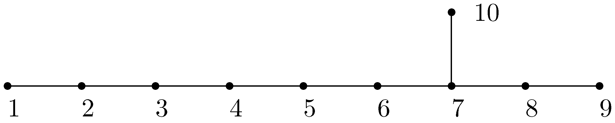
It may be verified that these sets do obey $E_{10}$ intersection rules following from the relations (61) (with $I_{s_i}=I_i$) and the Dynkin diagram from Figure 1.

Now, we present a cosmological S-brane solution from Section 4.2.1 for the configuration of ten branes under consideration. In what follows, the relations ${\epsilon }_s=+1$ and $h_s=1/2$, $s\in S$, are used.

The metric (127) reads:

$$\begin{array}{c}\hfill g={\left[{(\prod _{s\ne 7,10}{f}_s)}^4{f}_7^5{f}_{10}^{11}\right]}^{1/14}\{-e^{2c^{0}t+2{\overline{c}}^0}dt\otimes dt+{(f_2{f}_4{f}_6{f}_9{f}_{10})}^{-1}{e}^{2c^{1}t+2{\overline{c}}^1}d{x}^1\otimes d{x}^1\\ \hfill +{(f_4{f}_7{f}_{10})}^{-1}{e}^{2c^{2}t+2{\overline{c}}^2}d{x}^2\otimes d{x}^2+{(f_1{f}_4{f}_8{f}_{10})}^{-1}{e}^{2c^{3}t+2{\overline{c}}^3}d{x}^3\otimes d{x}^3\\ \hfill +{(f_1{f}_6{f}_{10})}^{-1}{e}^{2c^{4}t+2{\overline{c}}^4}d{x}^4\otimes d{x}^4+{(f_5{f}_{10})}^{-1}{e}^{2c^{5}t+2{\overline{c}}^5}d{x}^5\otimes d{x}^5\\ \hfill +{(f_2{f}_5{f}_8{f}_{10})}^{-1}{e}^{2c^{6}t+2{\overline{c}}^6}d{x}^6\otimes d{x}^6+{(f_2{f}_7{f}_{10})}^{-1}{e}^{2c^{7}t+2{\overline{c}}^7}d{x}^7\otimes d{x}^7\\ \hfill +{(f_3{f}_6{f}_8{f}_{10})}^{-1}{e}^{2c^{8}t+2{\overline{c}}^8}d{x}^8\otimes d{x}^8+{(f_3{f}_{10})}^{-1}{e}^{2c^{9}t+2{\overline{c}}^9}d{x}^9\otimes d{x}^9\\ \hfill +{(f_1{f}_3{f}_5{f}_7{f}_9{f}_{10})}^{-1}{e}^{2c^{10}t+2{\overline{c}}^{10}}d{x}^{10}\otimes d{x}^{10}+{(f_9{f}_{10})}^{-1}{e}^{2c^{11}t+2{\overline{c}}^{11}}d{x}^{11}\otimes d{x}^{11}\\ \hfill +{(\prod _{s=1}^9{f}_s)}^{-1}{e}^{2c^{12}t+2{\overline{c}}^{12}}d{x}^{12}\otimes d{x}^{12}+f_7^{-1}{e}^{2c^{13}t+2{\overline{c}}^{13}}d{x}^{13}\otimes d{x}^{13}\\ \hfill +e^{2c^{14}t+2{\overline{c}}^{14}}d{x}^{14}\otimes d{x}^{14}+e^{2c^{15}t+2{\overline{c}}^{15}}d{x}^{15}\otimes d{x}^{15}\}.\end{array}$$

(153)

For scalar fields (128), we get:

$$\begin{array}{c}\hfill {\phi }^{\alpha }=\frac{1}{2}[-{\lambda }_{5\alpha }(\sum _{s\ne 7,10}ln{f}_s)-{\lambda }_{6\alpha }ln{f}_7+{\lambda }_{4\alpha }ln{f}_{10}]+c_{\phi }^{\alpha }t+{\overline{c}}_{\phi }^{\alpha },\end{array}$$

(154)

$\alpha =1,\cdots ,5$ (here, we used the relations ${\lambda }_a^{\alpha }=-{\lambda }_{a\alpha }$).

The form fields (see (129) and (130)) are as follows:

$$\begin{array}{c}\hfill F^4=Q_{10}d{x}^{12}\wedge d{x}^{13}\wedge d{x}^{14}\wedge d{x}^{15},\end{array}$$

(155)

$$\begin{array}{c}\hfill F^5=Q_1{f}_1^{-2}{f}_{2}dt\wedge d{x}^3\wedge d{x}^4\wedge d{x}^{10}\wedge d{x}^{12}+Q_2{f}_1{f}_2^{-2}{f}_{3}dt\wedge d{x}^1\wedge d{x}^6\wedge d{x}^7\wedge d{x}^{12}\\ \hfill +Q_3{f}_2{f}_3^{-2}{f}_{4}dt\wedge d{x}^8\wedge d{x}^9\wedge d{x}^{10}\wedge d{x}^{12}+Q_4{f}_3{f}_4^{-2}{f}_{5}dt\wedge d{x}^1\wedge d{x}^2\wedge d{x}^3\wedge d{x}^{12}\\ \hfill +Q_5{f}_4{f}_5^{-2}{f}_{6}dt\wedge d{x}^5\wedge d{x}^6\wedge d{x}^{10}\wedge d{x}^{12}+Q_6{f}_5{f}_6^{-2}{f}_{7}dt\wedge d{x}^1\wedge d{x}^4\wedge d{x}^8\wedge d{x}^{12}\\ \hfill +Q_8{f}_7{f}_8^{-2}{f}_{9}dt\wedge d{x}^3\wedge d{x}^6\wedge d{x}^8\wedge d{x}^{12}+Q_9{f}_8{f}_9^{-2}dt\wedge d{x}^1\wedge d{x}^{10}\wedge d{x}^{11}\wedge d{x}^{12},\end{array}$$

(156)

$$\begin{array}{c}\hfill F^6=Q_7{f}_6{f}_7^{-2}{f}_8{f}_{10}dt\wedge d{x}^2\wedge d{x}^7\wedge d{x}^{10}\wedge d{x}^{12}\wedge d{x}^{13},\end{array}$$

(157)

where $Q_s\ne 0$, $s=1,\dots ,10$. Here:

$$c^0=\sum _{j=1}^{15}{c}^j,{\overline{c}}^0=\sum _{j=1}^{15}{\overline{c}}^j,$$

(158)

$f_s=exp(-q^s(t))$ and $q^s(t)$ obey Toda-type equations:

$$\ddot{q^s}=-2Q_s^{2}exp(\sum _{s^{\prime }=1}^{10}{A}_{s{s}^{\prime }}{q}^{s^{\prime }}),$$

(159)

$s=1,\dots ,10$, where $(A_{s{s}^{\prime }})$ is the Cartan matrix for the KM algebra $E_{10}$ (with the Dynkin diagram from Figure 1), and the energy integration constant:

$$E_T=\frac{1}{8}\sum _{s,s^{\prime }=1}^{10}{A}_{s{s}^{\prime }}\dot{q^s}\dot{q^{s^{\prime }}}+\frac{1}{2}\sum _{s=1}^{10}{Q}_s^{2}exp(\sum _{s^{\prime }=1}^{10}{A}_{s{s}^{\prime }}{q}^{s^{\prime }}),$$

(160)

obeys the constraint:

$$2E_T-\sum _{\alpha =1}^5{(c_{\phi }^{\alpha })}^2+\sum _{i=1}^{15}{(c^i)}^2-{\left(\sum _{i=1}^{15}{c}^i\right)}^2=0.$$

(161)

The brane constraints (109) are in our case:

$$\begin{array}{c}\hfill U^1(c)=c^3+c^4+c^{10}+c^{12}-\sum _{\alpha =1}^5{\lambda }_{5\alpha }{c}_{\phi }^{\alpha }=0,U^1(\overline{c})=0,\\ \hfill U^2(c)=c^1+c^6+c^7+c^{12}-\sum _{\alpha =1}^5{\lambda }_{5\alpha }{c}_{\phi }^{\alpha }=0,U^2(\overline{c})=0,\\ \hfill U^3(c)=c^8+c^9+c^{10}+c^{12}-\sum _{\alpha =1}^5{\lambda }_{5\alpha }{c}_{\phi }^{\alpha }=0,U^3(\overline{c})=0,\\ \hfill U^4(c)=c^1+c^2+c^3+c^{12}-\sum _{\alpha =1}^5{\lambda }_{5\alpha }{c}_{\phi }^{\alpha }=0,U^4(\overline{c})=0,\\ \hfill U^5(c)=c^5+c^6+c^{10}+c^{12}-\sum _{\alpha =1}^5{\lambda }_{5\alpha }{c}_{\phi }^{\alpha }=0,U^5(\overline{c})=0,\\ \hfill U^6(c)=c^1+c^4+c^8+c^{12}-\sum _{\alpha =1}^5{\lambda }_{5\alpha }{c}_{\phi }^{\alpha }=0,U^6(\overline{c})=0,\\ \hfill U^7(c)=c^2+c^7+c^{10}+c^{12}+c^{13}-\sum _{\alpha =1}^5{\lambda }_{6\alpha }{c}_{\phi }^{\alpha }=0,U^7(\overline{c})=0,\\ \hfill U^8(c)=c^3+c^6+c^8+c^{12}-\sum _{\alpha =1}^5{\lambda }_{5\alpha }{c}_{\phi }^{\alpha }=0,U^8(\overline{c})=0,\\ \hfill U^9(c)=c^1+c^{10}+c^{11}+c^{12}-\sum _{\alpha =1}^5{\lambda }_{5\alpha }{c}_{\phi }^{\alpha }=0,U^9(\overline{c})=0,\\ \hfill U^{10}(c)=\sum _{i=1}^{11}{c}^i+\sum _{\alpha =1}^5{\lambda }_{4\alpha }{c}_{\phi }^{\alpha }=0,U^{10}(\overline{c})=0.\\ \hfill \end{array}$$

(162)

Remark 5.

For a special choice of integration constants $c^i=0$ and $c_{\phi }^{\alpha }=0$, we get a solution governed by the $E_{10}$ Toda chain with the energy constraint $E_T=0$. According to the result from [30], we obtain a never ending asymptotical oscillating behavior of scale factors, which is described by the motion of a point-like particle in a billiard $B\subset H^9$. This billiard has a finite volume since $E_{10}$ is hyperbolic.

Special one-block solution: Now, we consider a special one-block solution (see Section 4.2.3). This solution is valid when a special set of charges is considered (see (149)):

$$Q_s^2=Q^2\left|b_s\right|,$$

(163)

where $Q\ne 0$ and [47]:

$$b_s=2\sum _{s^{\prime }=1}^{10}{A}^{s{s}^{\prime }}=-60,-122,-186,-252,-320,-390,-462,-306,-152,-230,$$

(164)

$s=1,\dots ,10$. Recall that $(A^{s{s}^{\prime }})={(A_{s{s}^{\prime }})}^{-1}$.

In this case, $f_s={(\overline{f})}^{b_s}$, where:

$$\begin{array}{c}\hfill \overline{f}(t)=\left|Q\right|\sqrt{2/C}sinh(\sqrt{C}(t-t_0)),C>0,\\ \hfill \left|Q\right|\sqrt{2/\left|C\right|}sin(\sqrt{\left|C\right|}(t-t_0)),C<0,\\ \hfill \left|Q\right|\sqrt{2}(t-t_0),C=0\end{array}$$

(165)

and $t_0$ is a constant.

From (150), we get:

$$E_T=-620C,$$

(166)

where relation ${\sum }_{s=1}^{10}{b}_s=-2480$ was used.

For the special solution under consideration, the electric monomials in (156) and (157) have a simpler form:

$${\mathcal{F}}^s=Q_s{\overline{f}}^{-2}dt\wedge \tau (I_s),$$

(167)

where $s=1,2,\dots ,9$.

Solution with one harmonic function: Let $C=0$ and all $c^i={\overline{c}}^i=0$, $c_{\phi }^{\alpha }={\overline{c}}_{\phi }^{\alpha }=0$. In this case, $H=\overline{f}(t)=\left|Q\right|\sqrt{2}(t-t_0)>0$ is a harmonic function on the one-dimensional manifold $((t_0,+\infty ),-dt\otimes dt)$, and our solution coincides with the one-block solution (51)–(55) (if $\mathrm{sign}{\nu }_s=-\mathrm{sign}{Q}_s$ for all s).

Example 4.

S-brane solution governed by $H{A}_2^{(1)}$ Toda chain.

Now, we consider the $B_{11}$-model in the 11-dimensional pseudo-Euclidean space of signature $(-,+,\dots ,+)$ with four-form $F^4$.

Here, we deal with four electric branes ($SM2$-branes) $s_1,s_2,s_3,s_4$ corresponding to the four-form $F^4$. The brane sets are the following ones: $I_1=\{1,2,3\}$, $I_2=\{4,5,6,\}$, $I_3=\{7,8,9\}$, $I_4=\{1,4,10\}$.

It may be verified that these sets obey the intersection rules corresponding to the hyperbolic KM algebra $H{A}_2^{(1)}$ with the following Cartan matrix:

$$\begin{array}{c}\hfill A=\left(\begin{array}{cccc}2& -1& -1& 0\\ -1& 2& -1& 0\\ -1& -1& 2& -1\\ 0& 0& -1& 2\end{array}\right),\end{array}$$

(168)

(see (61) with $I_{s_i}=I_i$).

Now, we give a cosmological S-brane solution from Section 4.2.1 for the configuration of four branes under consideration. In what follows, the relations ${\epsilon }_s=+1$ and $h_s=1/2$, $s\in S$, are used.

The metric (127) reads [117]:

$$\begin{array}{c}\hfill g={(f_1{f}_2{f}_3{f}_4)}^{1/3}\{-e^{2c^{0}t+2{\overline{c}}^0}dt\otimes dt+{(f_1{f}_4)}^{-1}{e}^{2c^{1}t+2{\overline{c}}^1}d{x}^1\otimes d{x}^1\\ \hfill +f_1^{-1}{e}^{2c^{2}t+2{\overline{c}}^2}d{x}^2\otimes d{x}^2+f_1^{-1}{e}^{2c^{3}t+2{\overline{c}}^3}d{x}^3\otimes d{x}^3\\ \hfill +{(f_2{f}_4)}^{-1}{e}^{2c^{4}t+2{\overline{c}}^4}d{x}^4\otimes d{x}^4+f_2^{-1}{e}^{2c^{5}t+2{\overline{c}}^5}d{x}^5\otimes d{x}^5\\ \hfill +f_2^{-1}{e}^{2c^{6}t+2{\overline{c}}^6}d{x}^6\otimes d{x}^6+f_3^{-1}{e}^{2c^{7}t+2{\overline{c}}^7}d{x}^7\otimes d{x}^7\\ \hfill +f_3^{-1}{e}^{2c^{8}t+2{\overline{c}}^8}d{x}^8\otimes d{x}^8+f_3^{-1}{e}^{2c^{9}t+2{\overline{c}}^9}d{x}^9\otimes d{x}^9\\ \hfill +f_4^{-1}{e}^{2c^{10}t+2{\overline{c}}^{10}}d{x}^{10}\otimes d{x}^{10}\}.\end{array}$$

(169)

The form field (see (129)) is as follows:

$$\begin{array}{c}\hfill F^4=Q_1{f}_1^{-2}{f}_2{f}_{3}dt\wedge d{x}^1\wedge d{x}^2\wedge d{x}^3+Q_2{f}_1{f}_2^{-2}{f}_{3}dt\wedge d{x}^4\wedge d{x}^5\wedge d{x}^6\\ \hfill +Q_3{f}_1{f}_2{f}_3^{-2}dt\wedge d{x}^7\wedge d{x}^8\wedge d{x}^9+Q_4{f}_3{f}_4^{-2}dt\wedge d{x}^1\wedge d{x}^4\wedge d{x}^{10},\end{array}$$

(170)

where $Q_s\ne 0$, $s=1,\dots ,4$. Here:

$$c^0=\sum _{j=1}^{10}{c}^j,{\overline{c}}^0=\sum _{j=1}^{10}{\overline{c}}^j,$$

(171)

$f_s=exp(-q^s(t))$ and $q^s(t)$ obey the Toda-type equations:

$$\ddot{q^s}=-2Q_s^{2}exp(\sum _{s^{\prime }=1}^4{A}_{s{s}^{\prime }}{q}^{s^{\prime }}),$$

(172)

$s=1,\dots ,4$, where $(A_{s{s}^{\prime }})$ is the Cartan matrix (168) for the KM algebra $H{A}_2^{(1)}$, and the energy integration constant:

$$E_T=\frac{1}{8}\sum _{s,s^{\prime }=1}^4{A}_{s{s}^{\prime }}\dot{q^s}\dot{q^{s^{\prime }}}+\frac{1}{2}\sum _{s=1}^4{Q}_s^{2}exp(\sum _{s^{\prime }=1}^4{A}_{s{s}^{\prime }}{q}^{s^{\prime }}),$$

(173)

obeys the constraint:

$$2E_T+\sum _{i=1}^{10}{(c^i)}^2-{\left(\sum _{i=1}^{10}{c}^i\right)}^2=0.$$

(174)

The brane constraints (109) read in this case as follows:

$$\begin{array}{c}\hfill U^1(c)=c^1+c^2+c^3=0,U^1(\overline{c})=0,\\ \hfill U^2(c)=c^4+c^5+c^6=0,U^2(\overline{c})=0,\\ \hfill U^3(c)=c^7+c^8+c^9=0,U^3(\overline{c})=0,\\ \hfill U^4(c)=c^1+c^4+c^{10}=0,U^4(\overline{c})=0,\end{array}$$

(175)

Since $F^4\wedge F^4=0$, this solution also obeys the equations of motion of 11-dimensional supergravity.

Special one-block solution. Now, we consider a special one-block solution (see Section 4.2.3). This solution is valid when a special set of charges is considered (see (149)):

$$Q_s^2=Q^2\left|b_s\right|,$$

(176)

where $Q\ne 0$ and:

$$b_s=2\sum _{s^{\prime }=1}^4{A}^{s{s}^{\prime }}=-12,-12,-14,-6.$$

(177)

In this case, $f_s={(\overline{f})}^{b_s}$, where $\overline{f}$ is the same as in (165).

For the energy integration constant, we have:

$$E_T=-11C,$$

(178)

(see (150)).

Example 5.

S-brane solution governed by $P_{10}$ Toda chain with $E_T=0$.

Now, we consider the $B_{11}$-model in the 11-dimensional pseudo-Euclidean space of signature $(-,+,\dots ,+)$ with four-form $F^4$.

Here, we deal with ten electric branes ($SM2$-branes) $s_1,\dots ,s_{10}$ corresponding to the four-form $F^4$. The brane sets are taken from [13,118] as: $I_1=\{1,4,7\}$, $I_2=\{8,9,10\}$, $I_3=\{2,5,7\}$, $I_4=\{4,6,10\}$, $I_5=\{2,3,9\}$, $I_6=\{1,2,8\}$, $I_7=\{1,3,10\}$, $I_8=\{4,5,8\}$, $I_9=\{3,6,7\}$, $I_{10}=\{5,6,9\}$.

These sets obey the intersection rules corresponding to the Lorentzian KM algebra $P_{10}$ (we call it Petersen algebra) with the following Cartan matrix:

$$\begin{array}{c}\hfill A=\left(\begin{array}{cccccccccc}2& -1& 0& 0& -1& 0& 0& 0& 0& -1\\ -1& 2& -1& 0& 0& 0& 0& 0& -1& 0\\ 0& -1& 2& -1& 0& 0& -1& 0& 0& 0\\ 0& 0& -1& 2& -1& -1& 0& 0& 0& 0\\ -1& 0& 0& -1& 2& 0& 0& -1& 0& 0\\ 0& 0& 0& -1& 0& 2& 0& 0& -1& -1\\ 0& 0& -1& 0& 0& 0& 2& -1& 0& -1\\ 0& 0& 0& 0& -1& 0& -1& 2& -1& 0\\ 0& -1& 0& 0& 0& -1& 0& -1& 2& 0\\ -1& 0& 0& 0& 0& -1& -1& 0& 0& 2.\end{array}\right),\end{array}$$

(179)

The Dynkin diagram for this Cartan matrix could be represented by the Petersen graph (“a star inside a pentagon”). $P_{10}$ is the Lorentzian KM algebra. It is a subalgebra of $E_{10}$ [13,118].

Let us present an S-brane solution for the configuration of 10 electric branes under consideration. The metric (127) reads [117]:

$$\begin{array}{c}\hfill g={\left(\prod _{s=1}^{10}{f}_s\right)}^{1/3}\{-dt\otimes dt+{(f_1{f}_6{f}_7)}^{-1}d{x}^1\otimes d{x}^1\\ \hfill +{(f_3{f}_5{f}_6)}^{-1}d{x}^2\otimes d{x}^2+{(f_5{f}_7{f}_9)}^{-1}d{x}^3\otimes d{x}^3\\ \hfill +{(f_1{f}_4{f}_8)}^{-1}d{x}^4\otimes d{x}^4+{(f_3{f}_8{f}_{10})}^{-1}d{x}^5\otimes d{x}^5\\ \hfill +{(f_4{f}_9{f}_{10})}^{-1}d{x}^6\otimes d{x}^6+{(f_1{f}_3{f}_9)}^{-1}d{x}^7\otimes d{x}^7\\ \hfill +{(f_2{f}_6{f}_8)}^{-1}d{x}^8\otimes d{x}^8+{(f_2{f}_5{f}_{10})}^{-1}d{x}^9\otimes d{x}^9\\ \hfill +{(f_2{f}_4{f}_7)}^{-1}d{x}^{10}\otimes d{x}^{10}\}.\end{array}$$

(180)

The form field (see (129)) is the following:

$$\begin{array}{c}\hfill F^4=Q_1{f}_1^{-2}{f}_2{f}_5{f}_{10}dt\wedge d{x}^1\wedge d{x}^4\wedge d{x}^7+Q_2{f}_1{f}_2^{-2}{f}_3{f}_{9}dt\wedge d{x}^8\wedge d{x}^9\wedge d{x}^{10}\\ \hfill +Q_3{f}_2{f}_3^{-2}{f}_4{f}_{7}dt\wedge d{x}^2\wedge d{x}^5\wedge d{x}^7+Q_4{f}_3{f}_4^{-2}{f}_5{f}_{6}dt\wedge d{x}^4\wedge d{x}^6\wedge d{x}^{10},\\ \hfill Q_5{f}_1{f}_4{f}_5^{-2}{f}_{8}dt\wedge d{x}^2\wedge d{x}^3\wedge d{x}^9+Q_6{f}_4{f}_6^{-2}{f}_9{f}_{10}dt\wedge d{x}^1\wedge d{x}^2\wedge d{x}^8\\ \hfill +Q_7{f}_3{f}_7^{-2}{f}_8{f}_{10}dt\wedge d{x}^1\wedge d{x}^3\wedge d{x}^{10}+Q_8{f}_5{f}_7{f}_8^{-2}{f}_{9}dt\wedge d{x}^4\wedge d{x}^5\wedge d{x}^8\\ \hfill Q_9{f}_2{f}_6{f}_8{f}_9^{-2}dt\wedge d{x}^3\wedge d{x}^6\wedge d{x}^7+Q_{10}{f}_1{f}_6{f}_7{f}_{10}^{-2}dt\wedge d{x}^5\wedge d{x}^6\wedge d{x}^9,\end{array}$$

(181)

where $Q_s\ne 0$, $s=1,\dots ,10$. Here, $f_s=exp(-q^s(t))$ and $q^s(t)$ obey the Toda-type equations:

$$\ddot{q^s}=-2Q_s^{2}exp(\sum _{s^{\prime }=1}^{10}{A}_{s{s}^{\prime }}{q}^{s^{\prime }})$$

(182)

where $(A_{s{s}^{\prime }})$ is the Cartan matrix (179) for the KM algebra $P_{10}$, and the energy constraint:

$$E_T=\frac{1}{8}\sum _{s,s^{\prime }=1}^4{A}_{s{s}^{\prime }}\dot{q^s}\dot{q^{s^{\prime }}}+\frac{1}{2}\sum _{s=1}^{10}{Q}_s^{2}exp(\sum _{s^{\prime }=1}^{10}{A}_{s{s}^{\prime }}{q}^{s^{\prime }})=0$$

(183)

is obeyed. Here, we used the fact that the two sets of linear equations—$U^s(c)=0$, $U^s(\overline{c})=0$, $s=1,\dots ,10$—have trivial solutions: $c=0$, $\overline{c}=0$, due to the linear independence of vectors $U^s$.

Since $F^4\wedge F^4=0$, this solution also obeys the equations of motion of 11-dimensional supergravity.

Remark 6.

As pointed out in [118], we do not obtain a never ending asymptotic oscillating behavior of the scale factors in this case, since the Lorentzian KM algebra $P_{10}$ is not hyperbolic, and the corresponding billiard $B\subset H^9$ has an infinite volume.

Special one-block solution. Now, we consider a special one-block solution. The calculations give us the following relations:

$$b_s=2\sum _{s^{\prime }=1}^{10}{A}^{s{s}^{\prime }}=-2,$$

(184)

$s=1,\dots ,10$ and hence, the special solution is valid (see (149)), when all charges are equal:

$$Q_s^2=Q^2,$$

(185)

where $Q\ne 0$. In this case, all $f_s={\overline{f}}^{-2}$, where:

$$\begin{array}{c}\hfill \overline{f}(t)=\left|Q\right|(t-t_0),\end{array}$$

(186)

and $t_0$ is constant. The metric (180) may be rewritten using the synchronous time variable $t_s$:

$$\begin{array}{c}\hfill g=-d{t}_s\otimes d{t}_s+A{t}_s^{2/7}\sum _{i=1}^{10}d{x}^i\otimes d{x}^i,\end{array}$$

(187)

where $A>0$ and $t_s>0$. This metric coincides with the power-law, inflationary solution in the model with a one-component perfect fluid when the following equation of state is adopted: $p=\frac{2}{5}\rho$, where p is pressure and $\rho$ is the density of fluid [119,120].

5. Black Brane Solutions

In this section, we consider the spherically-symmetric case of the metric (135), i.e., we put $w=1$, $M_1=S^{d_1}$, $g^1=d{\mathsf{\Omega }}_{d_1}^2$, where $d{\mathsf{\Omega }}_{d_1}^2$ is the canonical metric on a unit sphere $S^{d_1}$, $d_1\ge 2$. In this case, ${\xi }^1=d_1-1$. We put $M_2=\mathbb{R}$, $g^2=-dt\otimes dt$, i.e., $M_2$ is a time manifold.

Let $C_1\ge 0$. We consider solutions defined on some interval $[u_0,+\infty )$ with a horizon at $u=+\infty$.

When the matrix $(h_{\alpha \beta })$ is positive definite and:

$$2\in I_s,\forall s\in S,$$

(188)

i.e., all branes have a common time direction t, the horizon condition singles out the unique solution with $C_1>0$ and linear asymptotics at infinity:

$$q^s=-{\beta }^{s}u+{\overline{\beta }}^s+o(1),$$

(189)

$u\to +\infty$, where ${\beta }^s,{\overline{\beta }}^s$ are constants, $s\in S$ [51,52].

In this case:

$$\begin{array}{c}\hfill c^A/\overline{\mu }=-{\delta }_2^A+h_1{U}^{1A}+\sum _{s\in S}{h}_s{b}_s{U}^{sA},\end{array}$$

(190)

$$\begin{array}{c}\hfill {\beta }^s/\overline{\mu }=2\sum _{s^{\prime }\in S}{A}^{s{s}^{\prime }}\equiv b_s,\end{array}$$

(191)

where $s\in S$, $A=(i,\alpha )$, $\overline{\mu }=\sqrt{C_1}$, the matrix $(A^{s{s}^{\prime }})$ is inverse of the generalized Cartan matrix $(A_{s{s}^{\prime }})$ and $h_1={(U^1,U^1)}^{-1}=d_1/(1-d_1)$.

Let us introduce a new radial variable $R=R(u)$ through the relations:

$$\begin{array}{c}\hfill exp(-2\overline{\mu }u)=1-\frac{2\mu }{R^{\overline{d}}},\mu =\overline{\mu }/\overline{d}>0,\end{array}$$

(192)

where $u>0$, $R^{\overline{d}}>2\mu$, $\overline{d}=d_1-1$. We put ${\overline{c}}^A=0$ and $q^s(0)=0$, $A=(i,\alpha )$, $s\in S$. These relations guarantee the asymptotic flatness (for $R\to +\infty$) of the $(2+d_1)$-dimensional section of the metric.

Let us denote $H_s=f_s{e}^{-{\beta }^{s}u}$, $s\in S$. Then, Solutions (135)–(130) may be written as follows [50,51,52]:

$$\begin{array}{c}\hfill g=\left(\prod _{s\in S}{H}_s^{2h_{s}d(I_s)/(D-2)}\right)\{{\left(1-\frac{2\mu }{R^{\overline{d}}}\right)}^{-1}dR\otimes dR+R^{2}d{\mathsf{\Omega }}_{d_1}^2\\ \hfill -\left(\prod _{s\in S}{H}_s^{-2h_s}\right)\left(1-\frac{2\mu }{R^{\overline{d}}}\right)dt\otimes dt+\sum _{i=3}^n\left(\prod _{s\in S}{H}_s^{-2h_s{\delta }_{i{I}_s}}\right){\widehat{g}}^i\},\end{array}$$

(193)

$$\begin{array}{c}\hfill exp({\phi }^{\alpha })=\prod _{s\in S}{H}_s^{h_s{\chi }_s{\lambda }_{a_s}^{\alpha }},\end{array}$$

(194)

where $F^a={\sum }_{s\in S}{\delta }_{a_s}^a{\mathcal{F}}^s$, and:

$${\mathcal{F}}^s=-\frac{Q_s}{R^{d_1}}\left(\prod _{s^{\prime }\in S}{H}_{s^{\prime }}^{-A_{s{s}^{\prime }}}\right)dR\wedge \tau (I_s),$$

(195)

$s\in S_e$,

$${\mathcal{F}}^s=Q_s\tau ({\overline{I}}_s),$$

(196)

$s\in S_m$.

Here, $Q_s\ne 0$, $h_s=K_s^{-1}$, $s\in S$, and the generalized Cartan matrix $(A_{s{s}^{\prime }})$ is non-degenerate.

Functions $H_s>0$ obey the equations:

$$\frac{d}{dz}\left(\frac{(1-2\mu z)}{H_s}\frac{d}{dz}{H}_s\right)={\overline{B}}_s\prod _{s^{\prime }\in S}{H}_{s^{\prime }}^{-A_{s{s}^{\prime }}},$$

(197)

$$\begin{array}{c}\hfill H_s({(2\mu )}^{-1}-0)=H_{s0}\in (0,+\infty ),\end{array}$$

(198)

$$\begin{array}{c}\hfill H_s(+0)=1,\end{array}$$

(199)

$s\in S$, where $H_s(z)>0$, $\mu >0$, $z=R^{-\overline{d}}\in (0,{(2\mu )}^{-1})$ and ${\overline{B}}_s={\epsilon }_s{K}_s{Q}_s^2/{\overline{d}}^2\ne 0$.

There exist solutions to Equations (197)–(198) of the polynomial type. The simplest example occurs in the orthogonal case [55,65] (for $d_i=1$, see also [63,64]): $(U^s,U^{s^{\prime }})=0$, for $s\ne s^{\prime }$, $s,s^{\prime }\in S$. In this case, $(A_{s{s}^{\prime }})=\mathrm{diag}(2,\dots ,2)$ is a Cartan matrix for the semisimple Lie algebra ${\mathbf{A}}_{\mathbf{1}}\oplus \dots \oplus {\mathbf{A}}_{\mathbf{1}}$ and:

$$H_s(z)=1+P_{s}z$$

(200)

with $P_s\ne 0$, satisfying:

$$P_s(P_s+2\mu )=-{\overline{B}}_s,$$

(201)

$s\in S$.

In [107,108,121], this solution was generalized to a block-orthogonal case (46) and (47). In this case (200), is modified as follows:

$$H_s(z)={(1+P_{s}z)}^{b_s},$$

(202)

where $b_s$ are defined in (191) and parameters $P_s$ coincide inside blocks, i.e., $P_s=P_{s^{\prime }}$ for $s,s^{\prime }\in S_i$, $i=1,\cdots ,k$. The parameters $P_s\ne 0$ satisfy the relations [54,107,121]:

$$P_s(P_s+2\mu )=-{\overline{B}}_s/b_s,$$

(203)

$s\in S$, and the parameters ${\overline{B}}_s/b_s$ coincide inside blocks, i.e., ${\overline{B}}_s/b_s={\overline{B}}_{s^{\prime }}/b_{s^{\prime }}$ for $s,s^{\prime }\in S_i$, $i=1,\cdots ,k$.

For earlier supergravity solutions, see [122,123] and the references therein.

Finite-dimensional Lie algebras:

Let $(A_{s{s}^{\prime }})$ be a Cartan matrix for a finite-dimensional semisimple Lie algebra $\mathcal{G}$. In this case, all powers in (254) are natural numbers, which coincide with the components of twice the dual Weyl vector in the basis of simple co-roots [11], and hence, all functions $H_s$ are polynomials, $s\in S$.

Conjecture 1. Let $(A_{s{s}^{\prime }})$ be a Cartan matrix for a semisimple finite-dimensional Lie algebra $\mathcal{G}$. Then, the solutions to Equations (197)–(199) (if they exist) have a polynomial structure:

$$H_s(z)=1+\sum _{k=1}^{n_s}{P}_s^{(k)}{z}^k,$$

(204)

where $P_s^{(k)}$ are constants, $k=1,\dots ,n_s$; $n_s=b_s=2{\sum }_{s^{\prime }\in S}{A}^{s{s}^{\prime }}\in \mathbb{N}$ and $P_s^{(n_s)}\ne 0$, $s\in S$.

In the extremal case ($\mu =+0$), an analogue of this conjecture was suggested previously in [94]. Conjecture 1 was verified for the ${\mathbf{A}}_{\mathbf{m}}$ and ${\mathbf{C}}_{\mathbf{m}+\mathbf{1}}$ Lie algebras in [51,52]. Explicit expressions for polynomials corresponding to Lie algebras ${\mathbf{C}}_{\mathbf{2}}$ and ${\mathbf{A}}_{\mathbf{3}}$ were obtained in [124,125], respectively.

Remark 7.

In various notations, the $A_1$-solution with $H=1+\frac{P}{R}$ appeared earlier for dilatonic black hole solutions in [126] and [127,128] ($D=4$) and was extended to the multidimensional case in [127,128,129,130] (the results of [128] seem to be correct ones up to a typo in the first Formula (2.1) for the action in [128], which should be eliminated: the kinetic term for the scalar field should be multiplied by extra factor $1/2$). A special case with ${\lambda }^2=1/2$ (λ is dilatonic coupling) was considered earlier in [131,132].

Example 6.

Solution for $A_2$.

Here, we consider solutions related to the Lie algebra ${\mathbf{A}}_{\mathbf{2}}=sl(3)$ with the Cartan matrix

$$\left(A_{s{s}^{\prime }}\right)=\left(\begin{array}{cc}2& -1\\ -1& 2\end{array}\right).$$

(205)

According to the results of previous section, we seek the solutions to Equations (197)–(199) in the following form (see (204); here, $n_1=n_2=2$):

$$H_s=1+P_{s}z+P_s^{(2)}{z}^2,$$

(206)

where $P_s=P_s^{(1)}$ and $P_s^{(2)}\ne 0$ are constants, $s=1,2$.

From (197) we get for $P_1+P_2+4\mu \ne 0$ [50]:

$$\begin{array}{c}\hfill P_s^{(2)}=\frac{P_s{P}_{s+1}(P_s+2\mu )}{2(P_1+P_2+4\mu )},{\overline{B}}_s=-\frac{P_s(P_s+2\mu )(P_s+4\mu )}{P_1+P_2+4\mu },\end{array}$$

(207)

$s=1,2$. Here, we denote $s+1=2,1$ for $s=1,2$, respectively. For $P_1+P_2+4\mu =0$, we get a special (exceptional) solution with $P_1=P_2=-2\mu$, $2P_s^{(2)}={\overline{B}}_s>0$ and ${\overline{B}}_1+{\overline{B}}_2=4{\mu }^2$.

Thus, in the ${\mathbf{A}}_{\mathbf{2}}$-case, the non-exceptional solution is described by Relations (193)–(196) with $S=\{s_1,s_2\}$ (identified with $\{1,2\})$, intersection rules:

$$\begin{array}{c}\hfill d(I_{s_1}\cap I_{s_2})=\Delta (s_1,s_2)-K,\end{array}$$

(208)

where symbol $\Delta (s_1,s_2)$ is defined in (60) and $K=K_{s_i}=(U^{s_i},U^{s_i})\ne 0$; functions $H_{s_i}=H_i$ are defined by Relations (206) and (207) with $z=R^{-\overline{d}}$, $i=1,2$.

The $4d$ dilatonic dyon solution corresponding to the Lie algebra ${\mathbf{A}}_{\mathbf{2}}$ [51] (with ${\lambda }^2=3/2$, where $\lambda$ is dilatonic coupling) after Kaluza–Klein uplift to $D=5$ gives us the well-known Gibbons–Wiltshire solution [133], which is in an agreement with the general spherically-symmetric dyon solution (related to $A_2$ Toda chain) from [134].

${\mathbf{A}}_{\mathbf{2}}$-dyon in $\mathbf{D}=\mathbf{11}$ supergravity: Let us consider dyonic black-hole solutions with electric two-brane and magnetic five-brane defined on the manifold:

$$M=(2\mu ,+\infty )\times (M_1=S^2)\times (M_2=\mathbb{R})\times M_3\times M_4,$$

(209)

where $dim{M}_3=2$ and $dim{M}_4=5$. The solution reads,

$$\begin{array}{c}\hfill g=H_1^{1/3}{H}_2^{2/3}\{\frac{dR\otimes dR}{1-2\mu /R}+R^{2}d{\mathsf{\Omega }}_2^2\\ \hfill -H_1^{-1}{H}_2^{-1}\left(1-\frac{2\mu }{R}\right)dt\otimes dt+H_1^{-1}{\widehat{g}}^3+H_2^{-1}{\widehat{g}}^4\},\end{array}$$

(210)

$$\begin{array}{c}\hfill F=-\frac{Q_1}{R^2}{H}_1^{-2}{H}_{2}dR\wedge dt\wedge {\widehat{\tau }}_3+Q_2{\widehat{\tau }}_1\wedge {\widehat{\tau }}_3,\end{array}$$

(211)

where metrics $g^2$ and $g^3$ are Ricci-flat metrics of Euclidean signature, and $H_s$ are defined by (206), where $z=R^{-1}$ and parameters $P_s$, $P_s^{(2)}$, ${\overline{B}}_s=B_s=-2Q_s^2$, $s=1,2$, satisfy (207).

The solution describes the ${\mathbf{A}}_{\mathbf{2}}$-dyon consisting of electric two-brane with world volume isomorphic to $(M_2=\mathbb{R})\times M_3$ and magnetic five-brane with world volume isomorphic to $(M_2=\mathbb{R})\times M_4$. The “branes” are intersecting on the time manifold $M_2=\mathbb{R}$. Here, $K_s=(U^s,U^s)=2$, ${\epsilon }_s=-1$ for all $s\in S$. In our notations, the ${\mathbf{A}}_{\mathbf{2}}$ intersection rule reads: $3\cap 6=1$.

The field configurations (210) and (211) also satisfies to equations of motion for $D=11$ supergravity (in this case, $F\wedge F=0$). This solution in a special case $H_1=H_2=H^2$ ($P_1=P_2$, $Q_1^2=Q_2^2$) was considered in [121]. The four-dimensional section of the metric (210) in this special case coincides with the Reissner–Nordström metric. In the extremal case, $\mu \to +0$, the multi-black-hole generalization was considered in [46].

It should be noted that black hole solutions corresponding to Lie algebras ${\mathbf{A}}_{\mathbf{n}}=sl(n+1)$ were considered in [135].

Hyperbolic KM algebras: Let $(A_{s{s}^{\prime }})$ be a Cartan matrix for an infinite-dimensional hyperbolic KM algebra $\mathcal{G}$. In this case, all powers in (191) are negative numbers, and hence, we have no chance to get a polynomial structure for $H_s$. Here, we are led to an open problem of seeking solutions to the set of “master” Equations (197)–(198). These solutions define special solutions to Toda-chain equations corresponding to the hyperbolic KM algebra $\mathcal{G}$.

Example 7.

Black hole solutions for $A_1\oplus A_1$, $A_2$ and $H_2(q,q)$ KM algebras.

Let us consider the four-dimensional model governed by the action:

$$\begin{array}{c}\hfill S={\int }_M{d}^{4}z\sqrt{\left|g\right|}\{R[g]-\epsilon g^{MN}{\partial }_M\phi {\partial }_N\phi -\frac{1}{2}{e}^{2\lambda \phi }{(F^1)}^2-\frac{1}{2}{e}^{-2\lambda \phi }{(F^2)}^2\}.\end{array}$$

(212)

Here, $F^1$ and $F^2$ are two-forms, $\phi$ the scalar field, and $\epsilon =\pm 1$.

We consider a black brane solution defined on ${\mathbb{R}}_{*}\times S^2\times \mathbb{R}$ with two electric branes $s_1$ and $s_2$ corresponding to forms $F^1$ and $F^2$, respectively, with the sets $I_1=I_2=\{2\}$. Here, ${\mathbb{R}}_{*}$ is the subset of $\mathbb{R}$, $M_1=S^2$, $g^1=d{\mathsf{\Omega }}_2^2$, the canonical metric on $S^2$, $M_2=\mathbb{R}$, $g^2=-dt\otimes dt$ and ${\epsilon }_1={\epsilon }_2=-1$.

The scalar products of U-vectors are (we identify $U^i=U^{s_i}$):

$$\begin{array}{c}\hfill (U^1,U^1)=(U^2,U^2)=\frac{1}{2}+\epsilon {\lambda }^2\ne 0,(U^1,U^2)=\frac{1}{2}-\epsilon {\lambda }^2.\end{array}$$

(213)

The matrix A from (58) is a generalized non-degenerate Cartan matrix if and only if:

$$\frac{2(U^1,U^2)}{(U^2,U^2)}=-q,$$

(214)

or equivalently,

$$\epsilon {\lambda }^2=\frac{2+q}{2(2-q)},$$

(215)

where $q=0,1,3,4,...$. This takes place when:

$$\begin{array}{c}\hfill \epsilon =+1,q=0,1,\end{array}$$

(216)

$$\begin{array}{c}\hfill \epsilon =-1,q=3,4,5,\dots \end{array}$$

(217)

and:

$${\lambda }^2=\frac{2+q}{2|2-q|}.$$

(218)

The first branch ($\epsilon =+1$) corresponds to finite dimensional Lie algebras $A_1\oplus A_1$ ($q=0$), $A_2$ ($q=1$), and the second one ($\epsilon =-1$) corresponds to hyperbolic KM algebras $H_2(q,q)$, $q=3,4,...$. In the hyperbolic case, the scalar field $\phi$ is a phantom (ghost).

The black brane solution reads (see (193)–(195)):

$$\begin{array}{c}\hfill g={(H_1{H}_2)}^h\{{\left(1-\frac{2\mu }{R}\right)}^{-1}dR\otimes dR+R^{2}d{\mathsf{\Omega }}_2^2\\ \hfill -{(H_1{H}_2)}^{-2h}\left(1-\frac{2\mu }{R}\right)dt\otimes dt\},\end{array}$$

(219)

$$\begin{array}{c}\hfill exp(\phi )={(H_1/H_2)}^{\epsilon \lambda h},\end{array}$$

(220)

$$\begin{array}{c}\hfill F^s=\frac{Q_s}{R^2}{H}_s^{-2}{(H_{\overline{s}})}^{q}dt\wedge dR,\end{array}$$

(221)

$s=1,2$. Here, $h=(2-q)/2$ and $\overline{s}=2,1$ for $s=1,2$, respectively.

The moduli functions $H_s>0$ obey the Equations (see (197)):

$$\frac{d}{dz}\left(\frac{(1-2\mu z)}{H_s}\frac{d}{dz}{H}_s\right)=\frac{2Q_s^2}{q-2}{H}_s^{-2}{(H_{\overline{s}})}^q,$$

(222)

with the boundary conditions $H_s({(2\mu )}^{-1}-0)=H_{s0}\in (0,+\infty )$, $H_s(+0)=1$, $s=1,2$, imposed. Here, $\mu >0$, $z=1/R\in (0,{(2\mu )}^{-1})$. For $q=0,1$, the solutions to Equations (222) with the boundary conditions imposed were given in [50,51,52]. They are polynomials of degrees one and two for $q=0$ and $q=1$, respectively. For $q=3,4,\cdots$, the exact solutions to Equation (222) are not known yet.

Special solution with ${\mathbf{Q}}_{\mathbf{1}}^{\mathbf{2}}={\mathbf{Q}}_{\mathbf{2}}^{\mathbf{2}}$:

Now, we consider the special one-block solution from (202) and (201). Since $b_s=2/(2-q)$ and ${\overline{B}}_s=2Q_s^2/(q-2)$, it takes place when $Q_1^2=Q_2^2=Q^2>0$. The moduli functions read:

$$H_s=H^{2/(2-q)},H=1+Pz,$$

(223)

where $z=1/R$ and $q\ne 2$. These functions obey $H_s(z)>0$ for $z\in [0,{(2\mu )}^{-1}]$ if $P>-2\mu$ ($\mu >0$). Due to this inequality and the relation $P(P+2\mu )=Q^2$ (following from (203)), we get:

$$P=-\mu +\sqrt{{\mu }^2+Q^2}>0.$$

(224)

In this special case, the solution (219)–(221) has the following form:

$$\begin{array}{c}\hfill g=H^2\{{\left(1-\frac{2\mu }{R}\right)}^{-1}dR\otimes dR+R^{2}d{\mathsf{\Omega }}_2^2\\ \hfill -H^{-4}\left(1-\frac{2\mu }{R}\right)dt\otimes dt\},\end{array}$$

(225)

$$\begin{array}{c}\hfill \phi =0,\end{array}$$

(226)

$$\begin{array}{c}\hfill F^s=\frac{Q_s}{H^2{R}^2}dt\wedge dR,\end{array}$$

(227)

$s=1,2$. Remarkably, this special solution does not depend on q. The metric (225) coincides with the metric of the Reissner–Nordström solution (when the Maxwell two-form is $F=\sqrt{2}Q{(HR)}^{-2}dt\wedge dR$).

In the extremal case $\mu \to +0$, we are led to the special case of a Majumdar–Papapetrou-type solution:

$$\begin{array}{c}\hfill g=H^2{\widehat{g}}^0-H^{-2}dt\otimes dt,\end{array}$$

(228)

$$\begin{array}{c}\hfill \phi =0,\end{array}$$

(229)

$$\begin{array}{c}\hfill F^s={\nu }_{s}d{H}^{-1}\wedge dt,\end{array}$$

(230)

where $g^0={\sum }_{i=1}^{3}d{x}^i\otimes d{x}^i$, H is a harmonic function on $M_0={\mathbb{R}}^3$ and ${\nu }_s^2=1$, $s=1,2$. Here, ${\nu }_s=-Q_s/Q$.

Example 8.

Black brane solution corresponding to the KM algebra $H{A}_2^{(1)}=A_2^{++}$.

Now, we consider the $B_{15}$-model in 15-dimensional pseudo-Euclidean space of signature $(-,+,...,+)$ with the forms $F^4$,..., $F^8$.

Here, we deal with four electric branes $s_1,s_2,s_3,s_4$ corresponding to the six-form $F^6$. The brane sets are: $I_1=\{1,2,3,11,12\}$, $I_2=\{4,5,6,11,12\}$, $I_3=\{7,8,9,11,12\}$, $I_4=\{1,4,10,11,12\}$.

It may be verified that these sets obey the intersection rules corresponding to the hyperbolic KM algebra $H{A}_2^{(1)}$ with the Cartan matrix (168) (see (61) with $I_{s_i}=I_i$).

Now, we give a black brane solution for the configuration of four branes under consideration.

In what follows, the relations ${\epsilon }_s=+1$ and $h_s=1/2$, $s\in S$, are used.

The metric (193) reads [136]:

$$\begin{array}{c}\hfill g={(H_1{H}_2{H}_3{H}_4)}^{5/13}\{{\left(1-\frac{2\mu }{R}\right)}^{-1}dR\otimes dR+R^{2}d{\mathsf{\Omega }}_2^2\\ \hfill -{(H_1{H}_2{H}_3{H}_4)}^{-1}\left[\left(1-\frac{2\mu }{R}\right)d{t}^1\otimes d{t}^1+d{t}^2\otimes d{t}^2\right]\\ \hfill +{(H_1{H}_4)}^{-1}d{x}^1\otimes d{x}^1+H_1^{-1}[d{x}^2\otimes d{x}^2+d{x}^3\otimes d{x}^3]\\ \hfill +{(H_2{H}_4)}^{-1}d{x}^4\otimes d{x}^4+H_2^{-1}[d{x}^5\otimes d{x}^5+d{x}^6\otimes d{x}^6]\\ \hfill +H_3^{-1}[d{x}^7\otimes d{x}^7+d{x}^8\otimes d{x}^8+d{x}^9\otimes d{x}^9]\\ \hfill +H_4^{-1}d{x}^{10}\otimes d{x}^{10}\}.\end{array}$$

(231)

Here, $t^1=x^{11}$ and $t^2=x^{12}$ are time-like variables. In this case, the $2\times 2$ gravitational mass matrix $(M_{ij})$ [137,138] is a degenerate one.

The non-zero form field is:

$$\begin{array}{c}\hfill F^6=-Q_1{R}^{-2}{H}_1^{-2}{H}_2{H}_{3}dR\wedge d{t}^1\wedge d{t}^2\wedge d{x}^1\wedge d{x}^2\wedge d{x}^3\\ \hfill -Q_2{R}^{-2}{H}_1{H}_2^{-2}{H}_{3}dR\wedge d{t}^1\wedge d{t}^2\wedge d{x}^4\wedge d{x}^5\wedge d{x}^6\\ \hfill -Q_3{R}^{-2}{H}_1{H}_2{H}_3^{-2}{H}_{4}dR\wedge d{t}^1\wedge d{t}^2\wedge d{x}^7\wedge d{x}^8\wedge d{x}^9\\ \hfill -Q_4{R}^{-2}{H}_3{H}_4^{-2}dR\wedge d{t}^1\wedge d{t}^2\wedge d{x}^1\wedge d{x}^4\wedge d{x}^{10},\end{array}$$

(232)

where $Q_s\ne 0$, $s=1,2,3,4$.

The scalar fields read:

$${\phi }^{\alpha }=-\frac{1}{2}{\lambda }_{6\alpha }ln(H_1{H}_2{H}_3{H}_4),$$

(233)

$\alpha =1,2,3,4$. Here, $H_s>0$ obey the equations:

$$\frac{d}{dz}\left(\frac{(1-2\mu z)}{H_s}\frac{d}{dz}{H}_s\right)=2Q_s^2\prod _{s^{\prime }=1}^4{H}_{s^{\prime }}^{-A_{s{s}^{\prime }}},$$

(234)

with the boundary conditions $H_s({(2\mu )}^{-1}-0)=H_{s0}\in (0,+\infty )$ and $H_s(+0)=1$, $s=1,...,4$. Here, $\mu >0$, $z=R^{-1}\in (0,{(2\mu )}^{-1})$ and $(A_{s{s}^{\prime }})$ is the Cartan matrix (168) for the KM algebra $H{A}_2^{(1)}$.

Special one-block solution: This solution is valid when a special set of charges is considered:

$$Q_s^2=Q^2\left|b_s\right|,$$

(235)

where $Q\ne 0$ and:

$$b_s=2\sum _{s^{\prime }=1}^4{A}^{s{s}^{\prime }}=-12,-12,-14,-6,$$

(236)

for $s=1,2,3,4$, respectively. In this case, the moduli functions read:

$$H_s=H^{b_s},H=1+P/R,$$

(237)

where $P(P+2\mu )=2Q^2$. These functions obey $H>0$ for $R\in [2\mu ,+\infty )$ if $P>-2\mu$ ($\mu >0$). Due to this inequality and the relation $P(P+2\mu )=Q^2$, we get:

$$P=-\mu +\sqrt{{\mu }^2+2Q^2}>0.$$

(238)

The Hawking temperature in this case is [54] $T_H={(1+P/2\mu )}^{22}/(8\pi \mu )$. It diverges as $\mu \to +0$. This is in agreement with the fact that the metric (231) has a singularity at $R=+0$ if $\mu =+0$.

Example 9.

Black brane solution corresponding to the Lorentzian KM algebra $P_{10}$.

Now, we consider another solution for the $B_{15}$-model in 15-dimensional pseudo-Euclidean space of signature $(-,+,...,+)$ with the non-zero six-form $F^6$.

Here, we deal with ten electric branes $s_1,...,s_{10}$ corresponding to the four-form $F^4$. The brane sets are: $I_1=\{1,4,7,11,12\}$, $I_2=\{8,9,10,11,12\}$, $I_3=\{2,5,7,11,12\}$, $I_4=\{4,6,10,11,12\}$, $I_5=\{2,3,9,11,12\}$, $I_6=\{1,2,8,11,12\}$, $I_7=\{1,3,10,11,12\}$, $I_8=\{4,5,8,11,12\}$, $I_9=\{3,6,7,11,12\}$, $I_{10}=\{5,6,9,11,12\}$.

These sets obey the intersection rules corresponding to the Lorentzian KM algebra $P_{10}$ (Petersen algebra) with the Cartan matrix (179).

Let us present a black brane solution for the configuration of 10 electric branes under consideration. The metric (193) reads [136]:

$$\begin{array}{c}\hfill g={\left(\prod _{s=1}^{10}{H}_s\right)}^{5/13}\{{\left(1-\frac{2\mu }{R}\right)}^{-1}dR\otimes dR+R^{2}d{\mathsf{\Omega }}_2^2\\ \hfill -{\left(\prod _{s=1}^{10}{H}_s\right)}^{-1}\left[\left(1-\frac{2\mu }{R}\right)d{t}^1\otimes d{t}^1+d{t}^2\otimes d{t}^2\right]\\ \hfill +{(H_1{H}_6{H}_7)}^{-1}d{x}^1\otimes d{x}^1\\ \hfill +{(H_3{H}_5{H}_6)}^{-1}d{x}^2\otimes d{x}^2+{(H_5{H}_7{H}_9)}^{-1}d{x}^3\otimes d{x}^3\\ \hfill +{(H_1{H}_4{H}_8)}^{-1}d{x}^4\otimes d{x}^4+{(H_3{H}_8{H}_{10})}^{-1}d{x}^5\otimes d{x}^5\\ \hfill +{(H_4{H}_9{H}_{10})}^{-1}d{x}^6\otimes d{x}^6+{(H_1{H}_3{H}_9)}^{-1}d{x}^7\otimes d{x}^7\\ \hfill +{(H_2{H}_6{H}_8)}^{-1}d{x}^8\otimes d{x}^8+{(H_2{H}_5{H}_{10})}^{-1}d{x}^9\otimes d{x}^9\\ \hfill +{(H_2{H}_4{H}_7)}^{-1}d{x}^{10}\otimes d{x}^{10}\}.\end{array}$$

(239)

The form field is:

$$\begin{array}{c}\hfill F^6=-Q_1{R}^{-2}{H}_1^{-2}{H}_2{H}_5{H}_{10}dR\wedge d{t}^1\wedge d{t}^2\wedge d{x}^1\wedge d{x}^4\wedge d{x}^7\\ \hfill -Q_2{R}^{-2}{H}_1{H}_2^{-2}{H}_3{H}_{9}dR\wedge d{t}^1\wedge d{t}^2\wedge d{x}^8\wedge d{x}^9\wedge d{x}^{10}\\ \hfill -Q_3{R}^{-2}{H}_2{H}_3^{-2}{H}_4{H}_{7}dR\wedge d{t}^1\wedge d{t}^2\wedge d{x}^2\wedge d{x}^5\wedge d{x}^7\\ \hfill -Q_4{R}^{-2}{H}_3{H}_4^{-2}{H}_5{H}_{6}dR\wedge d{t}^1\wedge d{t}^2\wedge d{x}^4\wedge d{x}^6\wedge d{x}^{10}\\ \hfill -Q_5{R}^{-2}{H}_1{H}_4{H}_5^{-2}{H}_{8}dR\wedge d{t}^1\wedge d{t}^2\wedge d{x}^2\wedge d{x}^3\wedge d{x}^9\\ \hfill -Q_6{R}^{-2}{H}_4{H}_6^{-2}{H}_9{H}_{10}dR\wedge d{t}^1\wedge d{t}^2\wedge d{x}^1\wedge d{x}^2\wedge d{x}^8\\ \hfill -Q_7{R}^{-2}{H}_3{H}_7^{-2}{H}_8{H}_{10}dR\wedge d{t}^1\wedge d{t}^2\wedge d{x}^1\wedge d{x}^3\wedge d{x}^{10}\\ \hfill -Q_8{R}^{-2}{H}_5{H}_7{H}_8^{-2}{H}_{9}dR\wedge d{t}^1\wedge d{t}^2\wedge d{x}^4\wedge d{x}^5\wedge d{x}^8\\ \hfill -Q_9{R}^{-2}{H}_2{H}_6{H}_8{H}_9^{-2}dR\wedge d{t}^1\wedge d{t}^2\wedge d{x}^3\wedge d{x}^6\wedge d{x}^7\\ \hfill -Q_{10}{R}^{-2}{H}_1{H}_6{H}_7{H}_{10}^{-2}dR\wedge d{t}^1\wedge d{t}^2\wedge d{x}^5\wedge d{x}^6\wedge d{x}^9,\end{array}$$

(240)

where $Q_s\ne 0$, $s=1,\cdots ,10$.

The scalar fields read:

$${\phi }^{\alpha }=-\frac{1}{2}{\lambda }_{6\alpha }ln\left(\prod _{s=1}^{10}{H}_s\right),$$

(241)

$\alpha =1,2,3,4$. Here, $H_s>0$ obey the equations:

$$\frac{d}{dz}\left(\frac{(1-2\mu z)}{H_s}\frac{d}{dz}{H}_s\right)=2Q_s^2\prod _{s^{\prime }=1}^{10}{H}_{s^{\prime }}^{-A_{s{s}^{\prime }}},$$

(242)

with the boundary conditions $H_s({(2\mu )}^{-1}-0)=H_{s0}\in (0,+\infty )$, and $H_s(+0)=1$, $s=1,...,10$. Here, $\mu >0$, $z=R^{-1}\in (0,{(2\mu )}^{-1})$, and $(A_{s{s}^{\prime }})$ is the Cartan matrix (179) for the KM algebra $P_{10}$.

Special one-block solution. Now, we consider a special one-block solution. This solution is valid if a special set of charges is considered: $Q_s^2=2Q^2$ ($Q\ne 0$) in agreement with (235) and:

$$b_s=2\sum _{s^{\prime }=1}^{10}{A}^{s{s}^{\prime }}=-2,$$

(243)

for $s=1,...,10$. In this case, the functions $H_s$ are:

$$H_s=H^{-2},H=1+P/R,$$

(244)

where $P(P+2\mu )=2Q^2$. As in the previous case, we get a well-defined solution for $P=-\mu +\sqrt{{\mu }^2+2Q^2}>0$ and $\mu >0$.

The Hawking temperature in this case has the following form: $T_H={(1+P/2\mu )}^{10}/(8\pi \mu )$. It is smaller than that in the previous example, but it also diverges as $\mu \to +0$. It is in agreement with the singularity of the metric (239) at $R=+0$ for $\mu =+0$.

6. Fluxbrane Solutions

6.1. Preliminary Notes

In past decades, there were many papers devoted to multidimensional generalizations of the well-known Melvin solution [139]; for exact solutions and their applications, see [67,126,128,133,140,141,142,143,144,145,146,147,148,149,150,151,152,153,154,155,156,157,158,159,160,161,162,163,164,165] and the references therein.

We remind that the original Melvin solution describes the gravitational field of a magnetic flux tube. In the works of Gibbons and Wiltshire [133] and Gibbons and Maeda [128], the Melvin solution was generalized to arbitrary dimensions (in [128] with the inclusion of dilaton), and hence, the simplest fluxbranes appeared (the term fluxbrane was suggested in [145]; the Melvin solution is currently denoted as $F1$).

In papers [142,143,144,145], devoted to the Kaluza–Klein–Melvin solution (e.g., non-perturbative instability and pair production of magnetically charged black holes), it was shown that F1-fluxbrane supported by the potential one-form has a nice interpretation as a modding of flat space in one dimension higher. This “modding” technique is widely used in the construction of new solutions in supergravitational models and also for various physical applications in string and M-theory: construction of exact string backgrounds [141], duality between $0A$ and $IIA$ string theories [147], the dielectric effect [150,151,153], construction of supersymmetric configurations [155,156], etc.

The “modding” technique may be also used for Fp-fluxbranes supported by forms of higher ranks (constructed by the use of one-forms). Another approach suggested in [67,146], which works for Fp-fluxbranes, is based on generating techniques for certain duality groups. An important result here is a construction by Chen, Gal’tsov and Sharakin [146] of intersecting $F6$ and $F3$ fluxbranes corresponding to M-branes in $D=11$ supergravity.

The third and the most direct method is based on solving of Einstein equations [148,149,154]. Here, we overview this approach using the p-brane solutions from [49] (for a review of p-brane solutions, see [7,54]). We remind that in [49], a family of p-brane “cosmological-type” solutions with nearly arbitrary (up to some restrictions) intersection rules were obtained (see Section 2). These solutions are defined up to solutions to Toda-type equations and contain as a special case a subclass of solutions with cylindrical symmetry. Here, we single out a subclass of generalized fluxbrane configurations related to Toda-type equations with certain asymptotical conditions imposed (Section 3). These fluxbrane solutions are governed by functions $H_s(z)>0$ defined on the interval $(0,z_0)$ and obeying a set of second order non-linear differential equations:

$$\frac{d}{dz}\left(\frac{z}{H_s}\frac{d}{dz}{H}_s\right)={\widehat{B}}_s\prod _{s^{\prime }\in S}{H}_{s^{\prime }}^{-A_{s{s}^{\prime }}},$$

(245)

with the following boundary conditions imposed: $H_s(+0)=1$, $s\in S$ (S is a non-empty set). In (245), all ${\widehat{B}}_s\ne 0$ are constants, and $(A_{s{s}^{\prime }})$ is a “quasi-Cartan” matrix ($A_{ss}=2$) coinciding with the Cartan one when intersections are related to Lie algebras. In most interesting examples, $z_0=+\infty$, and all ${\widehat{B}}_s>0$.

We remind that different equations occur for black brane solutions from [50,51,52] (see Section 5):

$$\frac{d}{dz}\left(\frac{(1-2\mu z)}{H_s}\frac{d}{dz}{H}_s\right)={\overline{B}}_s\prod _{s^{\prime }\in S}{H}_{s^{\prime }}^{-A_{s{s}^{\prime }}},$$

(246)

where $\mu >0$ is the extremality parameter, $z\in (0,{(2\mu )}^{-1})$ and all ${\overline{B}}_s\ne 0$, (in most interesting cases, ${\overline{B}}_s<0$). For black brane solutions, the finite limits (on a horizon) $H_s({(2\mu )}^{-1}-0)=H_{s0}>0$ exist.

We note that fluxbrane “master equations” (245) may be obtained from the black brane ones (246) in the limit $\mu \to \infty$. In [166], it was shown that black brane moduli functions may be obtained from fluxbrane ones at least for small enough charge densities. For different aspects of p-brane/fluxbrane correspondence, see [152,158].

6.2. The Choice of Parameters

In what follows, we put:

$$w=1,d_1=1,$$

(247)

i.e., the manifold $M_1$ is one-dimensional one and:

$$1\in I_s,\forall s\in S,$$

(248)

i.e., all branes contain the $M_1$-submanifold. We note that the restriction (R2) (32) is satisfied automatically due to (248).

Here, we restrict ourselves to solutions with linear asymptotics at infinity:

$$q^s=-{\beta }^{s}u+{\overline{\beta }}^s+o(1),$$

(249)

$u\to +\infty$, where ${\beta }^s,{\overline{\beta }}^s$ are constants, $s\in S$. This relation gives us an asymptotical solution to Toda type Equation (107) if:

$$\sum _{s^{\prime }\in S}{A}_{s{s}^{\prime }}{\beta }^{s^{\prime }}>0,$$

(250)

for all $s\in S$. In this case, the energy (112) reads:

$$E_T=\frac{1}{4}\sum _{s,s^{\prime }\in S}{h}_s{A}_{s{s}^{\prime }}{\beta }^s{\beta }^{s^{\prime }}.$$

(251)

We put:

$${\overline{c}}^A=0,{\overline{\beta }}^s=0.$$

(252)

$A=(i,\alpha )$, $s\in S$ (these relations guarantee the asymptotical flatness for $u\to +\infty$ of the two-dimensional section of the metric for $M_1=S^1$ and $g^1=d\varphi \otimes d\varphi$).

We also put:

$$\begin{array}{c}\hfill c^A=-{\delta }_1^A+\sum _{s\in S}{h}_s{\beta }^s{U}^{sA},\end{array}$$

(253)

$$\begin{array}{c}\hfill {\beta }^s=2\sum _{s^{\prime }\in S}{A}^{s{s}^{\prime }},\end{array}$$

(254)

where $s\in S$, $A=(i,\alpha )$, and the matrix $(A^{s{s}^{\prime }})$ is inverse to the matrix $(A_{s{s}^{\prime }})=(2(U^s,U^{s^{\prime }})/(U^{s^{\prime }},U^{s^{\prime }}))$. It may be verified that the constraints (109) and (132) are satisfied identically, due to the conditions (247) and (248).

Relations (253) and (254) look similar to analogous relations for black branes [51,52,54]; see Equations (190) and (191), which appear from the horizon condition.

6.3. The Main Solution

We introduce a new radial variable:

$$\begin{array}{c}\hfill exp(-u)=\rho \end{array}$$

(255)

and denote:

$$H_s=f_s{e}^{-{\beta }^{s}u}=e^{-q^s-{\beta }^{s}u},$$

(256)

$s\in S$. Then, the solutions (10)–(12) may be written as follows [159]:

$$\begin{array}{c}\hfill g=\left(\prod _{s\in S}{H}_s^{2h_{s}d(I_s)/(D-2)}\right)\{d\rho \otimes d\rho \\ \hfill +\left(\prod _{s\in S}{H}_s^{-2h_s}\right){\rho }^2{\widehat{g}}^1+\sum _{i=2}^n\left(\prod _{s\in S}{H}_s^{-2h_s{\delta }_{i{I}_s}}\right){\widehat{g}}^i\},\end{array}$$

(257)

$$\begin{array}{c}\hfill exp({\phi }^{\alpha })=\prod _{s\in S}{H}_s^{h_s{\chi }_s{\lambda }_{a_s}^{\alpha }},\end{array}$$

(258)

$$\begin{array}{c}\hfill F^a=\sum _{s\in S}{\delta }_{a_s}^a{\mathcal{F}}^s,\end{array}$$

(259)

where:

$${\mathcal{F}}^s=-Q_s\left(\prod _{s^{\prime }\in S}{H}_{s^{\prime }}^{-A_{s{s}^{\prime }}}\right)\rho d\rho \wedge \tau (I_s),$$

(260)

$s\in S_e$,

$${\mathcal{F}}^s=Q_s\tau ({\overline{I}}_s),$$

(261)

$s\in S_m$.

Here, $Q_s\ne 0$, $h_s=K_s^{-1}$; parameters $K_s\ne 0$ and the non-degenerate matrix $(A_{s{s}^{\prime }})$ are defined by the relations:

$$(A_{s{s}^{\prime }})=\left(2B_{s{s}^{\prime }}/B_{s^{\prime }{s}^{\prime }}\right),$$

(262)

where:

$$B_{s{s}^{\prime }}\equiv d(I_s\cap I_{s^{\prime }})+\frac{d(I_s)d(I_{s^{\prime }})}{2-D}+{\chi }_s{\chi }_{s^{\prime }}{\lambda }_{\alpha a_s}{\lambda }_{\beta a_{s^{\prime }}}{h}^{\alpha \beta },$$

(263)

$s,s^{\prime }\in S$, with $(h^{\alpha \beta })={(h_{\alpha \beta })}^{-1}$.

Here, we assume that:

$$(i)B_{ss}\ne 0,$$

(264)

for all $s\in S$, and:

$$(ii)\det (B_{s{s}^{\prime }})\ne 0,$$

(265)

i.e., the matrix $(B_{s{s}^{\prime }})$ is a non-degenerate one.

Functions $H_s>0$ obey the equations:

$$\frac{d}{\rho d\rho }\left(\frac{\rho }{H_s}\frac{d{H}_s}{d\rho }\right)=B_s\prod _{s^{\prime }\in S}{H}_{s^{\prime }}^{-A_{s{s}^{\prime }}},$$

(266)

$s\in S$, where $B_s\ne 0$ are defined in (108). These equations follow from Toda-type Equation (107) and the definitions (255) and (256).

It follows from (249), (252) and (256) that there exist finite limits:

$$H_s\to 1,$$

(267)

$s\in S$, for $\rho \to 0$.

For the cylindrically-symmetric case:

$$M_1=S^1,g^1=d\varphi \otimes d\varphi ,$$

(268)

$0<\varphi <2\pi$, we get a family of composite fluxbrane solutions. They are defined up to solutions to radial Equation (266) with the boundary conditions (267) imposed. We note that the conic singularity for $\rho =+0$ is absent due to (267), and the metric is smooth if all moduli functions are positive.

In the next subsections, we consider several exact solutions to Equations (266) and (267).

Another possibility:

$$M_1=\mathbb{R},g^1=-dt\otimes dt,$$

(269)

$-\infty <t<+\infty$ (t is a time variable), will lead us to the generalized Milne-type solution.

6.4. Fluxbrane Intersection Rules

The fluxbrane submanifold (world volume) is isomorphic to $M({\overline{I}}_s)$ and has the following dimension:

$$d({\overline{I}}_s)=D-1-d(I_s),$$

(270)

$s\in S$; see (20)–(23). The fluxbrane intersection rules read:

$$d({\overline{I}}_s\cap {\overline{I}}_{s^{\prime }})=D-1-d(I_s)-d(I_{s^{\prime }})+d(I_s\cap I_{s^{\prime }}),$$

(271)

$s\ne s^{\prime }$, with p-brane intersections defined in (262). This relation follows from the identity:

$${\overline{I}}_s\cap {\overline{I}}_{s^{\prime }}=I_0\setminus (I_s\cup I_{s^{\prime }}),$$

(272)

see (56).

We note that here we use p-brane notations for the description of flux p-branes or $Fp$-branes. An electric (magnetic) p-brane corresponds to a magnetic (electric) $F(D-3-p)$ fluxbrane.

6.5. Polynomial Structure of $H_s$ for Finite-Dimensional Semi-Simple Lie Algebras

Now, we deal with solutions to second order non-linear differential Equation (266) that may be rewritten as follows:

$$\frac{d}{dz}\left(\frac{z}{H_s}\frac{d}{dz}{H}_s\right)=\frac{1}{4}{B}_s\prod _{s^{\prime }\in S}{H}_{s^{\prime }}^{-A_{s{s}^{\prime }}},$$

(273)

where $H_s(z)>0$, $s\in S$, $z={\rho }^2$. Equation (267) reads:

$$H_s(z=+0)=1,$$

(274)

$s\in S$.

In general, one may try to seek solutions of (273) in a class of functions analytical in some disc $\left|z\right|<L$:

$$H_s(z)=1+\sum _{k=1}^{\infty }{P}_s^{(k)}{z}^k,$$

(275)

where $P_s^{(k)}$ are constants, $s\in S$. Substitution of (275) into (273) gives us an infinite chain of relations on parameters $P_s^{(k)}$ and $B_s$. The first relation in this chain:

$$P_s\equiv P_s^{(1)}=\frac{1}{4}{B}_s,$$

(276)

$s\in S$, corresponds to the $z^0$-term in the decomposition of (273). For analytical function $H_s(z)$ (275) ($z={\rho }^2$), the metric (257) is regular at $\rho =0$.

Orthogonal case: Meanwhile, there exist solutions to Equations (273)–(274) of the polynomial type. The simplest example occurs in the orthogonal case, when:

$$(U^s,U^{s^{\prime }})=B_{s{s}^{\prime }}=0,$$

(277)

for $s\ne s^{\prime }$, $s,s^{\prime }\in S$. In this case, $(A_{s{s}^{\prime }})=\mathrm{diag}(2,\dots ,2)$ is a Cartan matrix for a semisimple Lie algebra $A_1\oplus \dots \oplus A_1$ and:

$$H_s(z)=1+P_{s}z,$$

(278)

with $P_s\ne 0$ satisfying (276) (for the $A_1$-case, see [154]).

Block-orthogonal case: The solution (278) may be generalized to so-called “block-orthogonal” (BO) case:

$$S=S_1\bigsqcup \cdots \bigsqcup S_k,$$

(279)

$S_i\ne \varnothing$, i.e., the set S is a union of k non-intersecting (non-empty) subsets $S_1,\cdots ,S_k$, and:

$$(U^s,U^{s^{\prime }})=0$$

(280)

for all $s\in S_i$, $s^{\prime }\in S_j$, $i\ne j$; $i,j=1,\cdots ,k$. For “block-orthogonal” black branes, see [108,121]. In this case, (278) is modified as follows:

$$H_s(z)={(1+{\overline{P}}_{s}z)}^{{\beta }^s},$$

(281)

where ${\beta }^s$ are defined in (254) and parameters ${\overline{P}}_s$ are coinciding inside blocks, i.e., ${\overline{P}}_s={\overline{P}}_{s^{\prime }}$ for $s,s^{\prime }\in S_i$, $i=1,\cdots ,k$, and satisfy the following relations:

$${\overline{P}}_s=B_s/(4{\beta }^s),$$

(282)

for ${\beta }^s\ne 0$, $s\in S$. In this case, $H_s$ are analytical in $\left|z\right|<L$, where $L=\min (|{\overline{P}}_s{|}^{-1},s\in S$).

Let $(A_{s{s}^{\prime }})$ be a Cartan matrix for a finite-dimensional semisimple Lie algebra $\mathcal{G}$. In this case, all powers in (191) are natural numbers:

$${\beta }^s=2\sum _{s^{\prime }\in S}{A}^{s{s}^{\prime }}=n_s\in \mathbb{N},$$

(283)

and hence, all functions $H_s$ are polynomials, $s\in S$. Integers $n_s$ coincide with the components of the twice dual Weyl vector in the basis of simple co-roots [11], which appeared earlier in Section 6.

Conjecture 2. Let $(A_{s{s}^{\prime }})$ be a Cartan matrix for a semisimple finite-dimensional Lie algebra $\mathcal{G}$. Then, the solution to Equations (273) and (274) (if exists) is a polynomial:

$$H_s(z)=1+\sum _{k=1}^{n_s}{P}_s^{(k)}{z}^k,$$

(284)

where $P_s^{(k)}$ are constants, $k=1,\dots ,n_s$, and integers $n_s$ are defined in (283) and $P_s^{(n_s)}\ne 0$, $s\in S$.

This conjecture may be verified for Lie algebras $A_m$, $C_{m+1}$ repeating all arguments from [51,52] for the black brane case with the replacement of $F(z)=1-2\mu z$ by $F(z)=z$.

6.6. Solutions for Lie Algebra $A_2$

Let us consider the Lie algebra $A_2=sl(3)$ with the Cartan matrix (205).

According to Conjecture 2, we seek the solutions to Equations (273)–(274) in the following form ($n_1=n_2=2$):

$$H_s=1+P_{s}z+P_s^{(2)}{z}^2,$$

(285)

where $P_s$ and $P_s^{(2)}\ne 0$ are constants, $s=1,2$.

The substitution of (285) into Equation (273) and decomposition in powers of z lead us to relations (276) and:

$$\begin{array}{c}\hfill P_s^{(2)}=\frac{1}{4}{P}_1{P}_2.\end{array}$$

(286)

Thus, in the $A_2$-case, the solution is described by relations (257)–(261) with $S=\{s_1,s_2\}$, p-brane intersection rules (262) or, equivalently,

$$\begin{array}{c}\hfill d(I_{s_1}\cap I_{s_2})=\frac{d(I_{s_1})d(I_{s_2})}{D-2}-{\chi }_{s_1}{\chi }_{s_2}{\lambda }_{a_{s_1}}·{\lambda }_{a_{s_2}}-\frac{1}{2}K,\end{array}$$

(287)

$$\begin{array}{c}\hfill d(I_{s_i})-\frac{{(d(I_{s_i}))}^2}{D-2}+{\lambda }_{a_{s_i}}·{\lambda }_{a_{s_i}}=K,\end{array}$$

(288)

where $K=K_{s_i}\ne 0$, and functions $H_{s_i}=H_i$ are defined by Relations (276), (285) and (286) with $z={\rho }^2$, $i=1,2$.

6.7. Examples of Fluxbrane Solutions

Here, we present certain examples of fluxbrane solutions with $M_1=S^1$ and $g^1=d\varphi \otimes d\varphi$. In all examples below, the total metric g has the signature $(-,+,\dots ,+)$, and all (p-brane) signature parameters are positive: ${\epsilon }_s=\epsilon (I_s)=+1$ (here, all ${\theta }_a=1$). In what follows, $0<\rho <+\infty$. In all examples, the metrics are regular at $\rho =0$.

6.7.1. Solutions for Algebra $A_1$

We start with single fluxbrane solutions ($S=\{s\}$).

Melvin solution ($F1$ fluxbrane): Let $D=4$, $n=3$, $M_2=\mathbb{R}$ with $g^2=-dt\otimes dt$ and $M_3=\mathbb{R}$ with $g^3=d\eta \otimes d\eta$, and $I_s=\{1\}$. The solution reads [139]:

$$\begin{array}{c}\hfill g=H^2\left\{d\rho \otimes d\rho +H^{-4}{\rho }^{2}d\varphi \otimes d\varphi -dt\otimes dt+d\eta \otimes d\eta \right\}.\end{array}$$

(289)

$$\begin{array}{c}\hfill F=-Q{H}^{-2}\rho d\rho \wedge d\varphi ,\end{array}$$

(290)

where $H=1+\frac{1}{8}{Q}^2{\rho }^2$. Here, $-Q$ is proportional to magnetic field in the core.

$\mathit{F}\mathbf{6}$ fluxbrane (corresponding to $\mathit{M}\mathbf{2}$-brane): Consider $D=11$ supergravity with the metric g and four-form F in the bosonic sector [2]. Let $n=3$, $M_3$ be a seven-dimensional (Ricci-flat) manifold with the metric $g^3=g_{\mu \nu }^{3}d{x}^{\mu }\otimes d{x}^{\nu }$ of signature $(-,+,\dots ,+)$ and $M_2$ be a two-dimensional (flat) manifold of signature $(+,+)$ with the metric $g^2=g_{mn}^{2}d{y}^m\otimes d{y}^n$ and $I_s=\{1,2\}$. The solution reads:

$$\begin{array}{c}\hfill g=H^{1/3}\left\{d\rho \otimes d\rho +H^{-1}({\rho }^{2}d\varphi \otimes d\varphi +{\widehat{g}}^2)+{\widehat{g}}^3\right\},\end{array}$$

(291)

$$\begin{array}{c}\hfill F=-Q{H}^{-2}\rho d\rho \wedge d\varphi \wedge {\widehat{\tau }}_2,\end{array}$$

(292)

where $H=1+\frac{1}{2}{Q}^2{\rho }^2$. For flat $g^3$, this solution was obtained earlier in [146].

$\mathit{F}\mathbf{3}$ fluxbrane (corresponding to $\mathit{M}\mathbf{5}$-brane): Now, we consider the solution dual to $F6$. Let $n=3$, $M_3$ be the four-dimensional (Ricci-flat) manifold with the metric $g^3=g_{\mu \nu }^{3}d{x}^{\mu }\otimes d{x}^{\nu }$ of signature $(-,+,+,+)$, and $M_2$ be the five-dimensional (Ricci-flat) manifold of signature $(+,\dots ,+)$ with the metric $g^2=g_{mn}^{2}d{y}^m\otimes d{y}^n$ and $I_s=\{1,2\}$. The solution reads:

$$\begin{array}{c}\hfill g=H^{2/3}\left\{d\rho \otimes d\rho +H^{-1}({\rho }^{2}d\varphi \otimes d\varphi +{\widehat{g}}^2)+{\widehat{g}}^3\right\},\end{array}$$

(293)

$$\begin{array}{c}\hfill F=Q{\widehat{\tau }}_3,\end{array}$$

(294)

where $H=1+\frac{1}{2}{Q}^2{\rho }^2$. For flat $g^2$ and $g^3$, see [146].

$\mathit{F}\mathbf{7},\mathit{F}\mathbf{6},\mathit{F}\mathbf{5}$ and $\mathit{F}\mathbf{1},\mathit{F}\mathbf{2},\mathit{F}\mathbf{3}$ fluxbranes in $\mathit{IIA}$ supergravity: The bosonic part of action for $D=10$$IIA$ supergravity reads:

$$S=\int d^{10}z\sqrt{\left|g\right|}\left\{R[g]-{(\partial \phi )}^2-\sum _{a=2}^4{e}^{2{\lambda }_a\phi }{(F^a)}^2\right\}-\frac{1}{2}\int F^4\wedge F^4\wedge A^2,$$

(295)

where $F^a=d{A}^{a-1}+{\delta }_4^a{A}^1\wedge F^3$ is an a-form, $a=2,3,4$, and:

$${\lambda }_2=3{\lambda }_4,{\lambda }_3=-2{\lambda }_4,{\lambda }_4^2=1/8.$$

(296)

The dimensions of p-brane world volumes are:

$$d=d(a,\chi )=\left\{\begin{array}{cc}1,2,3\hfill & inelectriccase,\chi =+1,\hfill \\ 7,6,5\hfill & inmagneticcase,\chi =-1,\hfill \end{array}\right.$$

(297)

for $a=2,3,4$, respectively.

The fluxbrane solutions read:

$$\begin{array}{c}\hfill g=H^{d/8}\left\{d\rho \otimes d\rho +H^{-1}{\rho }^{2}d\varphi \otimes d\varphi +H^{-1}{\widehat{g}}^2+{\widehat{g}}^3\right\},\end{array}$$

(298)

$$\begin{array}{c}\hfill exp(2\phi )=H^{\chi {\lambda }_a},\end{array}$$

(299)

and:

$$F^a=-Q{H}^{-2}\rho d\rho \wedge {\widehat{\tau }}_2,\mathrm{for}\chi =+1,$$

(300)

or

$$F^a=Q{\widehat{\tau }}_3,\mathrm{for}\chi =-1,$$

(301)

with $H=1+\frac{1}{2}{Q}^2{\rho }^2$, $a=2,3,4$.

For $\chi =+1$, we get a $F(9-a)$ fluxbrane with $d_2=a-2$, $d_3=10-a$, and for $\chi =-1$, we obtain a (dual) $F(a-1)$ fluxbrane with $d_2=8-a$, $d_3=a$, ($a=2,3,4$) (here, the presence of Chern–Simons terms does not modify the solutions from Section 6.3).

6.7.2. Solution for Algebra $A_1\oplus A_1$

$\mathit{F}\mathbf{6}\cap \mathit{F}\mathbf{3}$ fluxbranes. We put $n=5$, $d_2=1$, $g^2=d{y}^2\otimes d{y}^2$, $d_3=1$, $g^3=d{y}^3\otimes d{y}^3$, $d_4=4$; $g^4$ has the Euclidean signature, $d_5=3$; $g^5$ has the signature $(-,+,+)$; $I_{s_e}=\{1,2,3\}$ and $I_{s_m}=\{1,2,4\}$. The solution has the following form:

$$\begin{array}{c}\hfill g=H_e^{1/3}{H}_m^{2/3}\left\{d\rho \otimes d\rho +H_e^{-1}{H}_m^{-1}({\rho }^{2}d\varphi \otimes d\varphi +{\widehat{g}}^2)+H_e^{-1}{\widehat{g}}^3+H_m^{-1}{\widehat{g}}^4+{\widehat{g}}^5\right\},\end{array}$$

(302)

$$\begin{array}{c}\hfill F=-Q_e{H}_e^{-2}\rho d\rho \wedge d\varphi \wedge d{y}_2\wedge d{y}_3+Q_{m}d{y}_3\wedge {\widehat{\tau }}_5,\end{array}$$

(303)

where $H_s=1+\frac{1}{2}{Q}_s^2{\rho }^2$, $s=e,m$. For flat $g^i$, see [146].

6.7.3. Solutions for Algebra $A_2$

$\mathit{F}\mathbf{6}\cap \mathit{F}\mathbf{3}$ fluxbranes with ${\mathit{A}}_{\mathbf{2}}$-intersection: Now, we consider a new $F6\cap F3$ fluxbrane configuration with (a non-standard) $A_2$ intersection rules defined on the manifold:

$$M=(0,+\infty )\times M_1\times M_2\times M_3\times M_4,$$

(304)

where $d_2=2$, $d_3=5$, $d_4=2$. The solution is as follows:

$$\begin{array}{c}\hfill g=H_e^{1/3}{H}_m^{2/3}\left\{d\rho \otimes d\rho +H_e^{-1}{H}_m^{-1}{\rho }^{2}d\varphi \otimes d\varphi +H_e^{-1}{\widehat{g}}^2+H_m^{-1}{\widehat{g}}^3+{\widehat{g}}^4\right\},\end{array}$$

(305)

$$\begin{array}{c}\hfill F=-Q_e{H}_e^{-2}{H}_m\rho d\rho \wedge d\varphi \wedge {\widehat{\tau }}_2+Q_m{\widehat{\tau }}_2\wedge {\widehat{\tau }}_4,\end{array}$$

(306)

where metrics $g^2$ and $g^3$ are (Ricci-flat) metrics of Euclidean signature, $g^4$ is the (flat) metric of the signature $(-,+)$ and:

$$H_s=1+P_s{\rho }^2+\frac{1}{4}{P}_1{P}_2{\rho }^4,$$

(307)

where $P_s=\frac{1}{2}{Q}_s^2$, $s=e,m$.

Dyonic flux tube in Kaluza-Klein model: Let us consider the four-dimensional model:

$$S={\int }_M{d}^{4}z\sqrt{\left|g\right|}\left\{R[g]-g^{\mu \nu }{\partial }_{\mu }\phi {\partial }_{\nu }\phi -\frac{1}{2!}exp[2\lambda \phi ]F^2\right\}$$

(308)

with scalar field $\phi$, two-form $F=dA$ and $\lambda =-\sqrt{3/2}$. This model originates after Kaluza–Klein reduction of five-dimensional gravity. The five-dimensional metric in this case reads:

$$g^{(5)}=\mathsf{\Phi }{g}_{\mu \nu }d{x}^{\mu }\otimes d{x}^{\nu }+{\mathsf{\Phi }}^{-2}(dy+\mathcal{A})\otimes (dy+\mathcal{A}),$$

(309)

where:

$$\mathcal{A}=\sqrt{2}A=\sqrt{2}{A}_{\mu }d{x}^{\mu },\mathsf{\Phi }=exp(2\phi /\sqrt{6}).$$

(310)

We consider the “dyonic” flux-tube solution defined on the manifold:

$$M=(0,+\infty )\times (M_1=S^1)\times M_2,$$

(311)

where $M_2={\mathbb{R}}^2$ and $g^2=-dt\otimes dt+d\eta \otimes d\eta$. This solution reads:

$$\begin{array}{c}\hfill g={\left(H_e{H}_m\right)}^{1/2}\{d\rho \otimes d\rho -H_e^{-1}{H}_m^{-1}{\rho }^{2}d\varphi \otimes d\varphi -dt\otimes dt+d\eta \otimes d\eta \},\end{array}$$

(312)

$$\begin{array}{c}\hfill exp\phi =H_e^{\lambda /2}{H}_m^{-\lambda /2},\end{array}$$

(313)

$$\begin{array}{c}\hfill F=dA=-Q_e{H}_e^{-2}{H}_m\rho d\rho \wedge d\varphi +Q_{m}dt\wedge d\eta ,\end{array}$$

(314)

where functions $H_s$ are defined by Relations (307),

For the five-metric, we obtain from (309)–(313):

$$\begin{array}{c}\hfill g^{(5)}=H_m\{d\rho \otimes d\rho +H_e^{-1}{H}_m^{-1}{\rho }^{2}d\varphi \otimes d\varphi -dt\otimes dt+d\eta \otimes d\eta \}\\ \hfill +H_e{H}_m^{-1}(dy+\mathcal{A})\otimes (dy+\mathcal{A}),\end{array}$$

(315)

$d\mathcal{A}=\sqrt{2}F$. For $Q_m\to 0$, we get the solution from [128], and for $Q_e\to 0$, we are led to its dual version (see [146]).

6.8. Generalized Melvin Solution with Several Two-Forms

Now, we consider a generalization of the Melvin solution, which was presented earlier in [162]. It appears in the model that contains the metric, n Abelian two-forms and $l\ge n$ scalar fields. The action reads:

$$S=\int d^{D}x\sqrt{\left|g\right|}\left\{R[g]-h_{\alpha \beta }{g}^{MN}{\partial }_M{\phi }^{\alpha }{\partial }_N{\phi }^{\beta }-\frac{1}{2}\sum _{s=1}^{n}exp[2{\lambda }_s(\phi )]{(F^s)}^2\right\},$$

(316)

where $g=g_{MN}(x)d{x}^M\otimes d{x}^N$ is a metric, ${\phi }^{\alpha }$ are scalar fields, $\alpha =1,\cdots ,l$; $(h_{\alpha \beta })$ is symmetric non-degenerate $l\times l$ matrix, $F^s=d{A}^s=\frac{1}{2}{F}_{MN}^{s}d{z}^M\wedge d{z}^N$ are two-forms and ${\lambda }_s$ are linear functions: ${\lambda }_s(\phi )={\lambda }_{s\alpha }{\phi }^{\alpha }$, $s=1,\dots ,n$.

This solution is governed by a certain non-degenerate (quasi-Cartan) matrix $(A_{s{s}^{\prime }})$, $s,s^{\prime }=1,\cdots ,n$. It is a special case of the so-called generalized fluxbrane solutions from [159]; see Relations (257)–(259).

Here, we assume that $(A_{s{s}^{\prime }})$ is a Cartan matrix for some simple finite-dimensional Lie algebra $\mathcal{G}$ of rank n ($A_{ss}=2$ for all s). According to Conjecture 2 [159], the solutions to master Equation (245) with the boundary conditions imposed ($H_s(+0)=1$) are polynomials:

$$H_s(z)=1+\sum _{k=1}^{n_s}{P}_s^{(k)}{z}^k,$$

(317)

where $P_s^{(k)}$ are constants. Here, $P_s^{(n_s)}\ne 0$ and:

$$n_s=2\sum _{s^{\prime }=1}^n{A}^{s{s}^{\prime }},$$

(318)

where we denote $(A^{s{s}^{\prime }})={(A_{s{s}^{\prime }})}^{-1}$. Integers $n_s$ are components of a twice dual Weyl vector in the basis of simple (co-)roots [11].

We consider a family of exact solutions to field equations corresponding to the action (316) and depending on one variable $\rho$. The solutions are defined on the manifold:

$$M=(0,+\infty )\times M_1\times M_2,$$

(319)

where $M_1$ is a one-dimensional manifold (say $S^1$ or $\mathbb{R}$) and $M_2$ is a (D-2)-dimensional Ricci-flat manifold. The solution reads [162]:

$$\begin{array}{c}\hfill g=\left(\prod _{s=1}^n{H}_s^{2h_s/(D-2)}\right)\left\{wd\rho \otimes d\rho +\left(\prod _{s=1}^n{H}_s^{-2h_s}\right){\rho }^{2}d\varphi \otimes d\varphi +{\widehat{g}}^2\right\},\end{array}$$

(320)

$$\begin{array}{c}\hfill exp({\phi }^{\alpha })=\prod _{s=1}^n{H}_s^{h_s{\lambda }_s^{\alpha }},\end{array}$$

(321)

$$\begin{array}{c}\hfill F^s=q_s\left(\prod _{s^{\prime }=1}^n{H}_{s^{\prime }}^{-A_{s{s}^{\prime }}}\right)\rho d\rho \wedge d\varphi ,\end{array}$$

(322)

$s=1,\cdots ,n$; $\alpha =1,\cdots ,l$, where $w=\pm 1$, $g^1=d\varphi \otimes d\varphi$ is a metric on $M_1$ and $g^2$ is a Ricci-flat metric on $M_2$. Here, $q_s\ne 0$ are integration constants, $q_s=-Q_s$ in the notations of [162], $s=1,\cdots ,n$.

The functions $H_s(z)>0$, $z={\rho }^2$, obey the master equations:

$$\frac{d}{dz}\left(\frac{z}{H_s}\frac{d}{dz}{H}_s\right)=P_s\prod _{s^{\prime }=1}^n{H}_{s^{\prime }}^{-A_{s{s}^{\prime }}},$$

(323)

with the following boundary conditions:

$$H_s(+0)=1,$$

(324)

where:

$$P_s=\frac{1}{4}{K}_s{q}_s^2,$$

(325)

$s=1,\cdots ,n$.

The parameters $h_s$ satisfy the relations:

$$h_s=K_s^{-1},K_s=B_{ss}>0,$$

(326)

where:

$$B_{s{s}^{\prime }}\equiv 1+\frac{1}{2-D}+{\lambda }_{s\alpha }{\lambda }_{s^{\prime }\beta }{h}^{\alpha \beta },$$

(327)

$s,s^{\prime }=1,\dots ,n$, with $(h^{\alpha \beta })={(h_{\alpha \beta })}^{-1}$. In the relations above, we denote ${\lambda }_s^{\alpha }=h^{\alpha \beta }{\lambda }_{s\beta }$ and:

$$(A_{s{s}^{\prime }})=\left(2B_{s{s}^{\prime }}/B_{s^{\prime }{s}^{\prime }}\right).$$

(328)

It may be shown that if the matrix $(h_{\alpha \beta })$ has a Euclidean signature, $l\ge n$, and $(A_{s{s}^{\prime }})$ is a Cartan matrix for a simple Lie algebra $\mathcal{G}$ of rank n, there exists a set of co-vectors ${\lambda }_1,\cdots ,{\lambda }_n$ obeying (328). Thus, the solution is valid at least when $l\ge n$, and the matrix $(h_{\alpha \beta })$ is positive-definite.

The solution under consideration is a special case of the fluxbrane (for $w=+1$, $M_1=S^1$) and S-brane ($w=-1$) solutions from [159,161], respectively.

If $w=+1$ and the (Ricci-flat) metric $g_2$ has a pseudo-Euclidean signature, we get a multidimensional generalization of Melvin’s solution [139].

In our notations, Melvin’s solution (without the scalar field) corresponds to $D=4$, $n=1$, $l=0$, $M_1=S^1$ ($0<\varphi <2\pi$), $M_2={\mathbb{R}}^2$, $g_2=-dt\otimes dt+dx\otimes dx$ and $\mathcal{G}=A_1$.

For $w=-1$ and $g_2$ of the Euclidean signature, we obtain a cosmological solution with a horizon (as $\rho =+0$) if $M_1=\mathbb{R}$ ($-\infty <\varphi <+\infty$).

Flux integrals for simple finite-dimensional Lie algebras: Here, we deal with the solution that corresponds to a simple finite-dimensional Lie algebra $\mathcal{G}$, i.e., the matrix $A=(A_{s{s}^{\prime }})$ coincides with the Cartan matrix of this Lie algebra. We put also $n=l$, $w=+1$ and $M_1=S^1$, $h_{\alpha \beta }={\delta }_{\alpha \beta }$ and denote $({\lambda }_{sa})=({\lambda }_s^a)={\overrightarrow{\lambda }}_s$, $s=1,\cdots ,n$.

Due to (326)–(328), we get:

$$K_s=\frac{D-3}{D-2}+{\overrightarrow{\lambda }}_s^2,$$

(329)

$h_s=K_s^{-1}$, and

$${\overrightarrow{\lambda }}_s{\overrightarrow{\lambda }}_l=\frac{1}{2}{K}_l{A}_{sl}-\frac{D-3}{D-2},$$

(330)

$s,l=1,\cdots ,n$. ((329) is a special case of (330)).

Now, let us consider the oriented two-dimensional manifold $M_{*}=(0,+\infty )\times S^1$. The flux integrals:

$${\mathsf{\Phi }}^s={\int }_{M_{*}}{F}^s=2\pi {\int }_0^{+\infty }d\rho \rho {\mathcal{B}}^s,$$

(331)

where:

$${\mathcal{B}}^s=q_s\prod _{l=1}^n{H}_l^{-A_{sl}},$$

(332)

are convergent for all s, if the conjecture for the Lie algebra $\mathcal{G}$ (on polynomial structure of moduli functions $H_s$) is obeyed for the Lie algebra $\mathcal{G}$ under consideration.

Indeed, due to polynomial assumption (317), we have:

$$H_s\sim C_s{\rho }^{2n_s},C_s=P_s^{(n_s)},$$

(333)

as $\rho \to +\infty$; $s=1,\cdots ,n$. From (332) and (333) and the equality ${\sum }_1^n{A}_{sl}{n}_l=2$, following from (323), we get:

$${\mathcal{B}}^s\sim q_s{C}^s{\rho }^{-4},C^s=\prod _{l=1}^n{C}_l^{-A_{sl}},$$

(334)

and hence, the integral (331) is convergent for any $s=1,\cdots ,n$.

By using master Equation (323), we obtain:

$$\begin{array}{c}\hfill {\int }_0^{+\infty }d\rho \rho {\mathcal{B}}^s=q_s{P}_s^{-1}\frac{1}{2}{\int }_0^{+\infty }dz\frac{d}{dz}\left(\frac{z}{H_s}\frac{d}{dz}{H}_s\right)\\ \hfill =\frac{1}{2}{q}_s{P}_s^{-1}\underset{z\to +\infty }{lim}\left(\frac{z}{H_s}\frac{d}{dz}{H}_s\right)=\frac{1}{2}{n}_s{q}_s{P}_s^{-1},\end{array}$$

(335)

which implies (see (325)) [165]:

$${\mathsf{\Phi }}^s=4\pi n_s{q}_s^{-1}{h}_s,$$

(336)

$s=1,\cdots ,n$.

Thus, any flux ${\mathsf{\Phi }}^s$ depends on one integration constant $q_s\ne 0$, while the integrand form $F^s$ depends on all constants: $q_1,\cdots ,q_n$.

We note that for $D=4$ and $g^2=-dt\otimes dt+dx\otimes dx$, $q_s$ is coinciding with the value of the x-component of the magnetic field on the axis of symmetry.

Here, we present fluxbrane polynomials corresponding to Lie algebras $A_1$, $A_2$, $A_3$, $C_2$, $G_2$ and related fluxes. Here, as in [166], we use other parameters $p_s$ instead of $P_s$:

$$p_s=P_s/n_s,$$

(337)

$s=1,\dots ,n$.

${\mathit{A}}_{\mathbf{1}}$-case: The simplest example occurs in the case of the Lie algebra $A_1=sl(2)$. Here, $n_1=1$. We get [159]:

$$H_1=1+p_{1}z$$

(338)

and:

$${\mathsf{\Phi }}^1=4\pi q_1^{-1}{h}_1,$$

(339)

which is also valid for Melvin’s solution with $D=4$ and $h_1=2$.

${\mathit{A}}_{\mathbf{2}}$-case: For the Lie algebra $A_2=sl(3)$ with the Cartan matrix:

$$\left(A_{s{s}^{\prime }}\right)=\left(\begin{array}{cc}2& -1\\ -1& 2\end{array}\right)$$

(340)

we have [159,161,166] $n_1=n_2=2$ and:

$$\begin{array}{c}\hfill H_1=1+2p_{1}z+p_1{p}_2{z}^2,\end{array}$$

(341)

$$\begin{array}{c}\hfill H_2=1+2p_{2}z+p_1{p}_2{z}^2.\end{array}$$

(342)

We get in this case:

$$({\mathsf{\Phi }}^1,{\mathsf{\Phi }}^2)=8\pi h(q_1^{-1},q_2^{-1}),$$

(343)

where $h_1=h_2=h$.

${\mathit{A}}_{\mathbf{3}}$-case: The polynomials for the $A_3$-case read as follows [166,167]:

$$\begin{array}{c}\hfill H_1=1+3p_{1}z+3p_1{p}_2{z}^2+p_1{p}_2{p}_3{z}^3,\end{array}$$

(344)

$$\begin{array}{c}\hfill H_2=1+4p_{2}z+3\left(p_1{p}_2+p_2{p}_3\right)z^2+4p_1{p}_2{p}_3{z}^3+p_1{p}_2^2{p}_3{z}^4,\end{array}$$

(345)

$$\begin{array}{c}\hfill H_3=1+3p_{3}z+3p_2{p}_3{z}^2+p_1{p}_2{p}_3{z}^3.\end{array}$$

(346)

Here, we have $(n_1,n_2,n_3)=(3,4,3)$ and:

$$({\mathsf{\Phi }}^1,{\mathsf{\Phi }}^2,{\mathsf{\Phi }}^3)=4\pi h(3q_1^{-1},4q_2^{-1},3q_3^{-1})$$

(347)

with $h_1=h_2=h_2=h$.

${\mathit{C}}_{\mathbf{2}}$-case: For the Lie algebra $C_2=so(5)$ with the Cartan matrix:

$$\left(A_{s{s}^{\prime }}\right)=\left(\begin{array}{cc}2& -1\\ -2& 2\end{array}\right)$$

(348)

we get $n_1=3$ and $n_2=4$. For $C_2$-polynomials, we obtain [161,166]:

$$\begin{array}{c}\hfill H_1=1+3p_{1}z+3p_1{p}_2{z}^2+p_1^2{p}_2{z}^3,\end{array}$$

(349)

$$\begin{array}{c}\hfill H_2=1+4p_{2}z+6p_1{p}_2{z}^2+4p_1^2{p}_2{z}^3+p_1^2{p}_2^2{z}^4.\end{array}$$

(350)

In this case, we find:

$$({\mathsf{\Phi }}^1,{\mathsf{\Phi }}^2)=4\pi (3h_1{q}_1^{-1},4h_2{q}_2^{-1})$$

(351)

where $h_1=2h_2$.

${\mathit{G}}_{\mathbf{2}}$-case: For the Lie algebra $G_2$ with the Cartan matrix:

$$\left(A_{s{s}^{\prime }}\right)=\left(\begin{array}{cc}2& -1\\ -3& 2\end{array}\right)$$

(352)

we get $n_1=6$ and $n_2=10$. In this case, the fluxbrane polynomials read [161,166]:

$$\begin{array}{c}\hfill H_1=1+6p_{1}z+15p_1{p}_2{z}^2+20p_1^2{p}_2{z}^3+\\ \hfill 15p_1^3{p}_2{z}^4+6p_1^3{p}_2^2{z}^5+p_1^4{p}_2^2{z}^6,\end{array}$$

(353)

$$\begin{array}{c}\hfill H_2=1+10p_{2}z+45p_1{p}_2{z}^2+120p_1^2{p}_2{z}^3+p_1^2{p}_2(135p_1+75p_2)z^4\\ \hfill +252p_1^3{p}_2^2{z}^5+p_1^3{p}_2^2\left(75p_1+135p_2\right)z^6+120p_1^4{p}_2^3{z}^7\\ \hfill +45p_1^5{p}_2^3{z}^8+10p_1^6{p}_2^3{z}^9+p_1^6{p}_2^4{z}^{10}.\end{array}$$

(354)

We are led to relations:

$$({\mathsf{\Phi }}^1,{\mathsf{\Phi }}^2)=4\pi (6h_1{q}_1^{-1},10h_2{q}_2^{-1})$$

(355)

where $h_1=3h_2$.

Fluxbrane polynomials and fluxes, corresponding to the Lie algebra $E_6$, were calculated recently in [168].

Remark 8.

The relation for flux integrals (336) is also valid when the matrix $(A_{s{s}^{\prime }})$ is a Cartan matrix of a finite-dimensional semi-simple Lie algebra $\mathcal{G}={\mathcal{G}}_1\oplus \cdots \oplus {\mathcal{G}}_k$, where ${\mathcal{G}}_1,\cdots ,{\mathcal{G}}_k$ are simple Lie (sub)algebras. In this case, the Cartan matrix $(A_{ij})$ has a block-diagonal form, i.e., $(A_{ij})=\mathrm{diag}((A_{i_1{j}_1}^{(1)}),\cdots ,(A_{i_k{j}_k}^{(k)}))$, where $(A_{i_a{j}_a}^{(a)})$ is the Cartan matrix of the Lie algebra ${\mathcal{G}}_a$, $a=1,\cdots ,k$. The set of polynomials in this case splits in the direct union of sets of polynomials corresponding to Lie algebras ${\mathcal{G}}_1,\cdots ,{\mathcal{G}}_k$.

An open problem here is to study the convergence of flux integrals for non-polynomial solutions for moduli functions corresponding to non-Cartan matrices $(A_{s{s}^{\prime }})$, e.g., for the model with two two-forms from [169], see also [170,171,172,173] and the references therein.

7. Conclusions

Here, we reviewed several families of exact solutions in multidimensional gravity with a set of scalar fields and fields of forms related to non-singular (e.g., hyperbolic) KM algebras.

The solutions describe composite electromagnetic branes defined on warped products of Ricci-flat, or sometimes Einstein, spaces of arbitrary dimensions and signatures. The metrics are block-diagonal, and all scale factors, scalar fields and fields of forms depend on the points of some manifold $M_0$. The solutions include those depending on harmonic functions, S-branes and spherically-symmetric solutions (e.g., black-branes). Our approach is based on the sigma-model representation obtained in [56] under the rather general assumption of intersections of composite branes (when the stress-energy tensor has a diagonal structure).

We were dealing with rather general intersection rules [55] governed by the invertible generalized Cartan matrix corresponding to the certain generalized KM Lie algebra $\mathcal{G}$. For $\mathcal{G}={\mathbf{A}}_{\mathbf{1}}\oplus \cdots \oplus {\mathbf{A}}_{\mathbf{1}}$ (r terms), we get the well-known standard (e.g., supersymmetry preserving) intersection rules [56,60,61,62].

We have also considered a class of special “block-orthogonal” solutions corresponding to semisimple KM algebras and governed by several harmonic functions. Certain examples of one-block solutions (e.g., corresponding to KM algebras $H_2(q,q)$, $A{E}_3$) were considered.

In the one-block case, a generalization of the solutions to those governed by several functions of one harmonic function H and obeying Toda-type equations was presented.

For finite-dimensional (semi-simple) Lie algebras, we are led to integrable Lagrange systems, while the Toda chains corresponding to infinite-dimensional (non-singular) KM algebras are not well studied yet. Some examples of S-brane solutions corresponding to Lorentzian KM algebras $H{A}_2^{(1)}=A_2^{++}$, $E_{10}$ and $P_{10}$ were presented.

We have also considered general classes of cosmological-type solutions (e.g., S-brane and spherically-symmetric solutions) governed by Toda-type equations, containing black brane configurations as a special case. The “master” equations for moduli functions have polynomial solutions in the finite-dimensional case (according to our conjecture [50,51,52]), while in the infinite-dimensional case, we have only a special family of the so-called block-orthogonal solutions corresponding to semi-simple non-singular KM algebras. Examples of four-dimensional dilatonic black hole solutions corresponding to KM algebras $A_1\oplus A_1$, $A_2$ and $H_2(q,q)$ ($q>2$) were given.

We note that the problem of integrability of Toda chain equations corresponding to (non-singular) KM algebras arises also in the context of fluxbrane solutions [159] that have also a polynomial structure of moduli functions for finite-dimensional Lie algebras (see also [162]). (For similar S-brane solutions governed by polynomial functions and their applications in connection with cosmological problems, see [161,174,175].)

Here, we were dealing only with the case of non-degenerate matrix A. It is an open problem to find general classes of solutions with branes for the degenerate case when $\det$ A = 0 (e.g., corresponding to affine KM algebras). Some special solutions of such a type with the maximal set of composite electric S-branes (e.g., when A is not obviously a generalized Cartan matrix) were found in [176,177] and generalized in [178,179] for the arbitrary (anti-)self-dual parallel charge density form of dimension $2m$ defined on the Ricci-flat Riemannian sum-manifold of dimension $4m$. In these examples, the restrictions on brane intersections were replaced by more general condition on the stress-energy tensor: $T_N^M=0$, $M\ne N$.

Here, we have also presented a short review of a family of fluxbrane solutions with general intersection rules. The metrics of solutions contain n Ricci-flat metrics. The solutions are defined up to a set of “moduli” functions $H_s$ obeying a set of equations with the boundary conditions imposed. These solutions are new and generalize many special fluxbrane solutions considered earlier in the literature.

Here, we suggested a conjecture on polynomial structure of $H_s$ for intersections related to semisimple Lie algebras. This conjecture is valid for Lie algebras $A_m$ and $C_{m+1}$, $m\ge 1$, as may be verified with a little modification of the proof for the black brane case.

We have presented explicit formulas for $A_1\oplus \dots \oplus A_1$ (orthogonal), block-orthogonal and $A_2$ solutions. These formulas are illustrated by certain examples of solutions in $D=10,11$ supergravities (e.g., with $A_2$ intersection rules) and the Kaluza–Klein dyonic $A_2$ flux tube.

We have also considered the generalized Melvin solution for an arbitrary simple finite-dimensional Lie algebra $\mathcal{G}$. The solution contains metric, n Abelian two-forms and n scalar fields, where n is the rank of $\mathcal{G}$. It is governed by a set of n moduli functions $H_s(z)$ obeying n ordinary differential equations with certain boundary conditions imposed. As was conjectured earlier, these functions should be polynomials, the so-called fluxbrane polynomials, which depend on integration constants $q_s$, $s=1,\cdots ,n$. In the case when the conjecture on the polynomial structure for the Lie algebra $\mathcal{G}$ is satisfied, it is proven that two-form flux integrals ${\mathsf{\Phi }}^s$ over a proper $2d$ submanifold are finite and obey relations $q_s{\mathsf{\Phi }}^s=4\pi n_s{h}_s$, where $h_s>0$ are certain constants (related to dilatonic coupling vectors) and $n_s$ are powers of the polynomials, which are components of a twice dual Weyl vector in the basis of simple (co-)roots, $s=1,\cdots ,n$. Examples of polynomials and fluxes for Lie algebras $A_1$, $A_2$, $A_3$, $C_2$, $G_2$ are presented.

An open problem is to study the fluxes for the solutions related to infinite-dimensional Lorentzian Kac–Moody algebras, e.g., hyperbolic ones. In this case, one should deal with phantom scalar fields in the model and non-polynomial solutions to master equations for moduli functions. The methods considered in this paper may be used in the study of the mathematical aspects of the higher dimensional version of the modified gravity model [180,181,182] with several scalar fields and fields of forms.

References

- Staniukovich, K.P.; Melnikov, V.N. Hydrodynamics, Fields and Constants in the Theory of Gravitation; Energoatomizdat: Moscow, Russia, 1983. (In Russian) [Google Scholar]
- Cremmer, E.; Julia, B.; Scherk, J. Supergravity theory in eleven dimensions. Phys. Lett. B 1978, 76, 409–412. [Google Scholar] [CrossRef]
- Van Nieuwenhuizen, P. Supergravity. Phys. Rep. 1981, 68, 189–398. [Google Scholar] [CrossRef]
- Green, M.B.; Schwarz, J.H.; Witten, E. Superstring Theory; Cambridge University Press: Cambridge, UK, 1987. [Google Scholar]
- Hull, C.; Townsend, P. Unity of superstring dualities. Nucl. Phys. B 1995, 438, 109–137. [Google Scholar] [CrossRef]
- Witten, E. String theory dynamics in various dimensions. Nucl. Phys. B 1995, 443, 85–126. [Google Scholar] [CrossRef]
- Stelle, K.S. Lectures on supergravity p-branes. arXiv, 1997; arXiv:hep-th/9701088. [Google Scholar]
- Kac, V.G. Simple irreducible graded Lie algebras of finite growth. Izv. Akad. Nauk SSSR. Ser. Math. 1968, 32, 1323–1367. [Google Scholar] [CrossRef]
- Moody, R.V. A new class of Lie algebras. J. Algebra 1968, 10, 211–230. [Google Scholar] [CrossRef]
- Kac, V.G. Infinite-Dimensional Lie Algebras; Cambridge University Press: Cambridge, UK, 1990. [Google Scholar]
- Fuchs, J.; Schweigert, C. Symmetries, Lie Algebras and Representations. A Graduate Course for Physicists; Cambridge University Press: Cambridge, UK, 1997. [Google Scholar]
- Nikulin, V.V. On classification of hyperbolic systems of roots of rank 3. Procee. Steklov Inst. Math. 2000, 230, 241. (in Russian). [Google Scholar]
- Henneaux, M.; Persson, D.; Spindel, P. Spacelike Singularities and Hidden Symmetries of Gravity. Living Rev. Relativ. 2008, 11, 1. [Google Scholar] [CrossRef] [PubMed]
- Saçlioğlu, C. Dynkin diagram for hyperbolic Kac-Moody algebras. J. Phys. A 1989, 22, 3753–3769. [Google Scholar] [CrossRef]
- De Buyl, S.; Schomblond, C. Hyperbolic Kac Moody algebras and Einstein biliards. J. Math. Phys. 2004, 45, 4464–4492. [Google Scholar] [CrossRef]
- Carbone, L.; Chung, S.; Cobbs, L.; McRae, R.; Nandi, D.; Naqvi, Y.; Penta, D. Classification of hyperbolic Dynkin diagrams, root lengths and Weyl group orbits. J. Phys. A Math. Theor. 2010, 43, 155209–155223. [Google Scholar] [CrossRef]
- Feingold, A.; Frenkel, I.B. A hyperbolic Kac-Moody algebra and the theory of Siegel modular forms of genus 2. Math. Ann. 1983, 263, 87–144. [Google Scholar] [CrossRef]
- Julia, B. Lectures in Applied Mathematics. AMS-SIAM 1985, 21, 355. [Google Scholar]
- Mizoguchi, S. E10 Symmetry in One Dimensional Supergravity. Nucl. Phys. B 1998, 528, 238–264. [Google Scholar] [CrossRef]
- Nicolai, H. A hyperbolic Lie algebra from supergravity. Phys. Lett. B 1992, 276, 333–340. [Google Scholar] [CrossRef]
- Moore, G. String duality, automorphic forms, and generalized Kac-Moody algebras. Nucl. Phys. Proc. Suppl. 1998, 67, 56–67. [Google Scholar] [CrossRef]
- Damour, T.; Henneaux, M. E10, BE10 and Arithmetical Chaos in Superstring Cosmology. Phys. Rev. Lett. 2001, 86, 4749–4752. [Google Scholar] [CrossRef] [PubMed]
- Belinskii, V.A.; Lifshitz, E.M.; Khalatnikov, I.M. An oscillatory mode of approach to singularities in relativistic cosmology. Uspekhi Fiz. Nauk 1970, 102, 463. (In Russian); reprinted in Adv. Phys. 1982, 31, 639 [Google Scholar] [CrossRef]
- Damour, T.; Henneaux, M. Chaos in superstring cosmology. Phys. Rev. Lett. 2000, 85, 920. [Google Scholar] [CrossRef] [PubMed]
- Damour, T.; Henneaux, M.; Julia, B.; Nicolai, H. Hyperbolic Kac-Moody Algebras and Chaos in Kaluza-Klein Models. Phys. Lett. B 2001, 509, 323–330. [Google Scholar] [CrossRef]
- Chitré, D.M. Investigation of Vanishing of a Horizon for Bianchi Type IX (Mixmaster) Universe. Ph.D. Thesis, University of Maryland, College Park, MD, USA, 1972. [Google Scholar]
- Ivashchuk, V.D.; Kirillov, A.A.; Melnikov, V.N. On Stochastic Properties of Multidimensional Cosmological Models near the Singular Point. Izv. Vuzov (Fiz.) 1994, 11, 107. (In Russian); reprinted in Russ. Phys. J. 1994, 37, 1102 [Google Scholar]
- Ivashchuk, V.D.; Kirillov, A.A.; Melnikov, V.N. On Stochastic Behaviour of Multidimensional Cosmological Models near the Singularity. Pis’ma ZhETF 1994, 60, 225. (In Russian); reprinted in JETP Lett. 1994, 60, 235 [Google Scholar]
- Ivashchuk, V.D.; Melnikov, V.N. Billiard representation for multidimensional cosmology with multicomponent perfect fluid near the singularity. Class. Quantum Gravity 1995, 12, 809. [Google Scholar] [CrossRef]
- Ivashchuk, V.D.; Melnikov, V.N. Billiard Representation for Pseudo-Euclidean Toda-like Systems of Cosmological Origin. Regul. Chaotic Dyn. 1996, 1, 23–35. [Google Scholar]
- Ivashchuk, V.D.; Melnikov, V.N. Billiard representation for multidimensional cosmology with intersecting p-branes near the singularity. J. Math. Phys. 2000, 41, 6341–6363. [Google Scholar] [CrossRef]
- Damour, T.; Henneaux, M. Oscillatory behaviour in homogeneous string cosmology models. Phys. Lett. B 2000, 488, 108–116. [Google Scholar] [CrossRef]
- Damour, T.; Henneaux, M.; Nicolai, H. Cosmological billiards. Class. Quantum Gravity 2003, 20, R145–R200. [Google Scholar] [CrossRef]
- Ivashchuk, V.D.; Melnikov, V.N. On billiard approach in multidimensional cosmological models. Gravit. Cosmol. 2009, 15, 49–58. [Google Scholar] [CrossRef]
- Damour, T.; Henneaux, M.; Nicolai, H. E10 and a small tension expansion of M-theory. Phys. Rev. Lett. 2002, 89, 221601. [Google Scholar] [CrossRef] [PubMed]
- Gaberdiel, M.; Olive, D.; West, P. A class of Lorentzian Kac-Moody algebras. Nucl. Phys. B 2002, 645, 403–437. [Google Scholar] [CrossRef]
- West, P. E11 and M theory. Class. Quantum Gravity 2001, 18, 4443. [Google Scholar] [CrossRef]
- Schnakenburg, I.; West, P. Kac-Moody symmetries of IIB supergravity. Phys. Lett. B 2001, 517, 421–428. [Google Scholar] [CrossRef]
- Lambert, N.D.; West, P.C. Coset symmetries in dimensionally reduced bosonic string theory. Nucl. Phys. B 2001, 615, 117–132. [Google Scholar] [CrossRef]
- Englert, F.; Houart, L.; Taormina, A.; West, P. The symmetry of M-theories. J. High Energy Phys. 2003, 2003, 020. [Google Scholar] [CrossRef]
- Englert, F.; Houart, L.; West, P. Intersection Rules, Dynamics and Symmetries. J. High Energy Phys. 2003, 2003, 025. [Google Scholar] [CrossRef]
- Kleinschmidt, A.; Schnakenburg, I.; West, P. Very-extended Kac-Moody algebras and their interpretation at low levels. Class. Quantum Gravity 2004, 21, 2493–2525. [Google Scholar] [CrossRef]
- Kleinschmidt, A. E11 as E10 representation at low levels. Nucl. Phys. B 2003, 677, 553–586. [Google Scholar] [CrossRef]
- Englert, F.; Houart, L. G+++ invariant formulation of gravity and M-theories: Exact intersecting brane solutions. J. High Energy Phys. 2004, 2004, 059. [Google Scholar] [CrossRef]
- Bossard, G.; Kleinschmidt, A.; Palmkvist, J.; Pope, C.N.; Sezgin, E. Beyond E11. J. High Energy Phys. 2017, 5, 020. [Google Scholar] [CrossRef]
- Ivashchuk, V.D.; Melnikov, V.N. Majumdar-Papapetrou Type Solutions in Sigma-model and Intersecting p-branes. Class. Quantum Gravity 1999, 16, 849. [Google Scholar] [CrossRef]
- Grebeniuk, M.A.; Ivashchuk, V.D. Sigma-model solutions and intersecting p-branes related to Lie algebras. Phys. Lett. B 1998, 442, 125–135. [Google Scholar] [CrossRef]
- Ivashchuk, V.D.; Kim, S.-W.; Melnikov, V.N. Hyperbolic Kac-Moody algebra from intersecting p-branes. J. Math. Phys. 1998, 40, 4072–4083, Erratum in 2001, 42, 11. [Google Scholar] [CrossRef] [Green Version]
- Ivashchuk, V.D.; Kim, S.-W. Solutions with intersecting p-branes related to Toda chains. J. Math. Phys. 2000, 41, 444–460. [Google Scholar] [CrossRef]
- Ivashchuk, V.D.; Melnikov, V.N. P-brane black Holes for General Intersections. Gravit. Cosmol. 1999, 5, 313–318. [Google Scholar]
- Ivashchuk, V.D.; Melnikov, V.N. Black hole p-brane solutions for general intersection rules. Gravit. Cosmol. 2000, 6, 27–40. [Google Scholar]
- Ivashchuk, V.D.; Melnikov, V.N. Toda p-brane black holes and polynomials related to Lie algebras. Class. Quantum Gravity 2000, 17, 2073–2092. [Google Scholar] [CrossRef]
- Ivashchuk, V.D. Composite S-brane solutions related to Toda-type systems. Class. Quantum Gravity 2003, 20, 261–276. [Google Scholar] [CrossRef]
- Ivashchuk, V.D.; Melnikov, V.N. Exact solutions in multidimensional gravity with antisymmetric forms. Class. Quantum Gravity 2001, 18, R82–R157. [Google Scholar] [CrossRef]
- Ivashchuk, V.D.; Melnikov, V.N. Multidimensional classical and quantum cosmology with intersecting p-branes. J. Math. Phys. 1998, 39, 2866–2889. [Google Scholar] [CrossRef]
- Ivashchuk, V.D.; Melnikov, V.N. Sigma-model for the Generalized Composite p-branes. Class. Quantum Gravity 1997, 14, 3001–3029. [Google Scholar] [CrossRef]
- Ivashchuk, V.D.; Melnikov, V.N. Intersecting p-Brane Solutions in Multidimensional Gravity and M-Theory. Gravit. Cosmol. 1996, 2, 297–305. [Google Scholar]
- Ivashchuk, V.D.; Melnikov, V.N. Generalized intersecting p-brane solutions from the σ-model approach. Phys. Lett. B 1997, 403, 23–30. [Google Scholar] [CrossRef]
- Ivashchuk, V.D.; Melnikov, V.N.; Rainer, M. Multidimensional Sigma-Models with Composite Electric p-branes. Gravit. Cosmol. 1998, 4, 73–82. [Google Scholar]
- Aref’eva, I.Y.; Rytchkov, O.A. Incidence Matrix Description of Intersecting p-brane Solutions. Am. Math. Soc. Trans. 2000, 201, 19–38. [Google Scholar]
- Argurio, R.; Englert, F.; Hourant, L. Intersection rules for p-branes. Phys. Lett. B 1997, 398, 61–68. [Google Scholar] [CrossRef]
- Aref’eva, I.Y.; Ivanov, M.G.; Rytchkov, O.A. Properties of Intersecting p-branes in Various Dimensions. In Supersymmetry and Quantum Field Theory; Springer: Berlin/Heidelberg, Germany, 1998; pp. 25–41. [Google Scholar]
- Aref’eva, I.Y.; Ivanov, M.G.; Volovich, I.V. Non-extremal intersecting p-branes in various dimensions. Phys. Lett. B 1997, 406, 44–48. [Google Scholar] [CrossRef]
- Ohta, N. Intersection rules for non-extreme p-branes. Phys. Lett. B 1997, 403, 218–224. [Google Scholar] [CrossRef]
- Bronnikov, K.A.; Ivashchuk, V.D.; Melnikov, V.N. The Reissner-Nordström Problem for Intersecting Electric and Magnetic p-Branes. Gravit. Cosmol. 1997, 3, 203–212. [Google Scholar]
- Ivashchuk, V.D. On symmetries of Target Space for σ-model of p-brane Origin. Gravit. Cosmol. 1998, 4, 217–220. [Google Scholar]
- Gal’tsov, D.V.; Rytchkov, O.A. Generating Branes via Sigma models. Phys. Rev. D 1998, 58, 122001. [Google Scholar] [CrossRef]
- West, P. The IIA, IIB and eleven dimensional theories and their common E11 origin. Nucl. Phys. B 2004, 693, 76–102. [Google Scholar] [CrossRef]
- Tseytlin, A.A. Harmonic superposition of M-branes. Nucl. Phys. B 1996, 475, 149–163. [Google Scholar] [CrossRef]
- Gauntlett, J.P. Intersecting branes. In Proceedings of the February 97 APCTP Winter School on Dualities of Gauge and String Theories, Seoul, Korea, 17–28 February 1997. [Google Scholar]
- Bergshoeff, E.; de Roo, M.; Eyras, E.; Janssen, B.; van der Schaar, J.P. Multiple Intersections of D-branes and M-branes. Nucl. Phys. B 1997, 494, 119–143. [Google Scholar] [CrossRef]
- Tseytlin, A.A. “No-force” condition and BPS combinations of p-branes in 11 and 10 dimensions. Nucl. Phys. B 1997, 487, 141–154. [Google Scholar] [CrossRef]
- Gibbons, G.W.; Hawking, S.W. Action integrals and partition functions in quantum gravity. Phys. Rev. D 1977, 15, 2752. [Google Scholar] [CrossRef]
- Ivashchuk, V.D.; Melnikov, V.N.; Zhuk, A.I. On Wheeler-De Witt equation in multidimensional cosmology. Nuovo Cim. B 1989, 104, 575–587. [Google Scholar] [CrossRef]
- Nicolai, H.; Olive, D.I. The principal SO(1,2) subalgebra of a hyperbolic Kac-Moody algebra. Lett. Math. Phys. 2001, 58, 141–152. [Google Scholar] [CrossRef]
- Khviengia, N.; Khviengia, Z.; Lü, H.; Pope, C.N. Towards a field theory of F-theory. Class. Quantum Gravity 1998, 15, 759–773. [Google Scholar] [CrossRef]
- Vafa, C. Evidence for F-theory. Nucl. Phys. B 1996, 469, 403–415. [Google Scholar] [CrossRef]
- Majumdar, S.D. A Class of Exact Solutions of Einstein’s Field Equations. Phys. Rev. 1947, 72, 390. [Google Scholar] [CrossRef]
- Papapetrou, A. A static solution of the equations of the gravitational field for an. arbirtary charge distribution. Proc. R. Irish Acad. A 1947, 51, 191. [Google Scholar]
- Duff, M.; Stelle, K. Multimembrane solutions of D = 11 supergravity. Phys. Lett. B 1991, 253, 113–118. [Google Scholar] [CrossRef]
- Güven, R. Black p-brane solutions of D = 11 supergravity theory. Phys. Lett. B 1992, 276, 49–55. [Google Scholar] [CrossRef]
- Papadopoulos, G.; Townsend, P.K. Intersecting M-branes. Phys. Lett. B 1996, 380, 273–279. [Google Scholar] [CrossRef]
- Gauntlett, J.P.; Kastor, D.A.; Traschen, J. Overlapping branes in M-theory. Nucl. Phys. B 1996, 478, 544–560. [Google Scholar] [CrossRef]
- Ivashchuk, V.D. On supersymmetric solutions in D = 11 supergravity on product of Ricci-flat spaces. Gravit. Cosmol. 2000, 6, 344–350. [Google Scholar]
- Ivashchuk, V.D. More M-branes on product of Ricci-flat manifolds. Int. J. Geom. Methods Mod. Phys. 2012, 9, 1250067–1250093. [Google Scholar] [CrossRef]
- Golubtsova, A.A.; Ivashchuk, V.D. Triple M-brane solutions and supersymmetry. Tomsk State Pedag. Univ. Bull. 2012, 128, 53–58. [Google Scholar]
- Golubtsova, A.A.; Ivashchuk, V.D. Triple M-brane configurations and supersymmetries. Nucl. Phys. B 2013, 872, 289–312. [Google Scholar] [CrossRef]
- Ivashchuk, V.D. On Supersymmetric M-Brane Configurations with an R1,1/Z2 Submanifold. Gravit. Cosmol. 2016, 22, 32–35. [Google Scholar] [CrossRef]
- Ivashchuk, V.D.; Melnikov, V.N. Perfect-fluid Type Solution in Multidimensional Cosmology. Phys. Lett. A 1989, 136, 465–467. [Google Scholar] [CrossRef]
- Gavrilov, V.R.; Melnikov, V.N. Toda Chains with Type Am Lie Algebra for Multidimensional Classical Cosmology with Intersecting p-branes. In Proceedings of the International Seminar “Curent Topics in Mathematical Cosmology”, Potsdam, Germany, 30 March–4 April 1998; Rainer, M., Schmidt, H.-J., Eds.; World Scientific: Singapore, 1998; p. 310. [Google Scholar]
- Gavrilov, V.R.; Melnikov, V.N. Toda Chains Associated with Lie Algebras Am in Multidimensional Gravitation and Cosmology with Intersecting p-branes. Theor. Math. Phys. 2000, 123, 374–394. (In Russian) [Google Scholar]
- Lü, H.; Mukherji, S.; Pope, C.N.; Xu, K.-W. Cosmological Solutions in String Theories. Phys. Rev. D 1997, 55, 7926–7935. [Google Scholar] [CrossRef]
- Lü, H.; Pope, C.N.; Xu, K.W. Liouville and Toda Solitons in M-Theory. Mod. Phys. Lett. A 1996, 11, 1785–1796. [Google Scholar] [CrossRef]
- Lü, H.; Maharana, J.; Mukherji, S.; Pope, C.N. Cosmological Solutions, p-branes and the Wheeler De Witt Equation. Phys. Rev. D 1997, 57, 2219–2229. [Google Scholar] [CrossRef]
- Gutperle, M.; Strominger, A. Spacelike branes. J. High Energy Phys. 2002, 2002, 018. [Google Scholar] [CrossRef]
- Chen, C.M.; Gal’tsov, D.M.; Gutperle, M. S-brane solutions in supergravity theories. Phys. Rev. D 2002, 66, 024043. [Google Scholar] [CrossRef]
- Kruczenski, M.; Myers, R.C.; Peet, A.W. Supergravity S-branes. J. High Energy Phys. 2002, 2002, 039. [Google Scholar] [CrossRef]
- Roy, S. On supergravity solutions of space-like Dp-branes. J. High Energy Phys. 2002, 2002, 025. [Google Scholar] [CrossRef]
- Degger, N.S.; Kaya, A. Intersecting S-brane solutions of D = 11 supergravity. J. High Energy Phys. 2002, 2002, 038. [Google Scholar] [CrossRef]
- Ohta, N. Intersection rules for S-branes. Phys. Lett. B 2003, 558, 213–220. [Google Scholar] [CrossRef]
- Ivashchuk, V.D. On composite S-brane solutions with orthogonal intersection rules. arXiv, 2003; arXiv:hep-th/0309027. [Google Scholar]
- Ivashchuk, V.D. S-brane solutions with orthogonal intersection rules (invited paper to a fest of A. Garsia). Gen. Relativ. Gravit. 2012, 37, 751–758, Erratum in 2012, 44, 1101. [Google Scholar] [CrossRef]
- Ivashchuk, V.D.; Melnikov, V.N.; Selivanov, A.B. Composite S-brane solutions on product of Ricci-flat spaces. Gen. Relativ. Gravit. 2004, 36, 1593–1602. [Google Scholar] [CrossRef]
- Ivashchuk, V.D.; Melnikov, V.N.; Selivanov, A.B. Cosmological solutions in multidimensional model with multiple exponential potential. J. High Energy Phys. 2003, 2003, 059. [Google Scholar] [CrossRef]
- Ivashchuk, V.D.; Melnikov, V.N.; Kim, S.-W. S-brane solutions with acceleration, in models with forms and multiple exponential potential. arXiv, 2004; arXiv:hep-th/0405009. [Google Scholar]
- Ivashchuk, V.D.; Melnikov, V.N. Cosmological and Spherically Symmetric Solutions with Intersecting p-branes. J. Math. Phys. 1999, 40, 6558–6576. [Google Scholar] [CrossRef]
- Ivashchuk, V.D.; Melnikov, V.N. Multidimensional cosmological and spherically symmetric solutions with intersecting p-branes. In Lecture Notes in Physics, Proceedings of the Second Samos Meeting on Cosmology, Geometry and Relativity—Mathematical and Quantum Aspects of Relativity and Cosmology, Samos, Greece, 31 August–4 September 1998; Cotsakis, S., Gibbons, G.W., Eds.; Springer: Berlin, Germany, 2000; Volume 537. [Google Scholar]
- Bronnikov, K.A. Block-orthogonal Brane systems, Black Holes and Wormholes. Gravit. Cosmol. 1998, 4, 49–56. [Google Scholar]
- Toda, M. Waves in nonlinear lattice. Prog. Theor. Phys. 1970, 45, 174–200. [Google Scholar] [CrossRef]
- Bogoyavlensky, O.I. On perturbations of the periodic Toda lattice. Commun. Math. Phys. 1976, 51, 201–209. [Google Scholar] [CrossRef]
- Kostant, B. The solution to a generalized Toda lattice and representation theory. Adv. Math. 1979, 34, 195–338. [Google Scholar] [CrossRef]
- Olshanetsky, M.A.; Perelomov, A.M. Explicit solutions of classical generalized Toda models. Invent. Math. 1979, 54, 261–269. [Google Scholar] [CrossRef]
- Adler, M.; van Moerbeke, P. Kowalewski’s asymptotic method, Kac-Moody Lie algebras and regularization. Commun. Math. Phys. 1982, 83, 83–106. [Google Scholar] [CrossRef]
- Kozlov, V.V.; Treshchev, D.V. Polynomial integrals of Hamiltonian systems with exponential interaction. Math. USSR Izv. 1990, 34, 555–574. [Google Scholar] [CrossRef]
- Emel’yanov, K.V.; Tsygvintsev, A.V. Kovalevskaya exponents of systems with exponential interaction. Math. Sb. 2000, 191, 39–50. (In Russian) [Google Scholar] [CrossRef]
- Gebert, R.W.; Inami, T.; Mizoguchi, S. The Painleve Property, W Algebras and Toda Field Theories associated with Hyperbolic Kac-Moody Algebras. Int. J. Mod. Phys. A 1996, 11, 5479–5493. [Google Scholar] [CrossRef]
- Ivashchuk, V.D.; Melnikov, V.N. On brane solutions related to non-singular Kac-Moody algebras. SIGMA 2009, 5, 070–104. [Google Scholar] [CrossRef]
- Henneaux, M.; Leston, M.; Persson, D.; Spindel, P. Geometric Configurations, Regular Subalgebras of E10 and M-Theory Cosmology. J. High Energy Phys. 2006, 2006, 021. [Google Scholar] [CrossRef]
- Ivashchuk, V.D.; Melnikov, V.N. Multidimensional Classical and Quantum Cosmology with Perfect Fluid. Gravit. Cosmol. 1995, 1, 133–148. [Google Scholar]
- Alimi, J.-M.; Ivashchuk, V.D.; Kononogov, S.A.; Melnikov, V.N. Multidimensional cosmology with anisotropic fluid: Acceleration and variation of G. Gravit. Cosmol. 2006, 12, 173–178. [Google Scholar]
- Cotsakis, S.; Ivashchuk, V.D.; Melnikov, V.N. P-brane Black Holes and Post-Newtonian Approximation. Gravit. Cosmol. 1999, 5, 52–57. [Google Scholar]
- Cvetic, M.; Tseytlin, A. Non-extreme black holes from non-extreme intersecting M-branes. Nucl. Phys. B 1996, 478, 181–198. [Google Scholar] [CrossRef]
- Ohta, N.; Shimizu, T. Non-extreme Black Holes from Intersecting M-branes. Int. J. Mod. Phys. A 1998, 13, 1305–1328. [Google Scholar] [CrossRef]
- Grebeniuk, M.A.; Ivashchuk, V.D.; Kim, S.-W. Black-brane solutions for C2 algebra. J. Math. Phys. 2002, 43, 6016–6023. [Google Scholar] [CrossRef]
- Grebeniuk, M.A.; Ivashchuk, V.D.; Melnikov, V.N. Black-brane solution for A3 algebra. Phys. Lett. B 2002, 543, 98–106. [Google Scholar] [CrossRef]
- Bronnikov, K.A.; Shikin, G.N. On interacting fields in general relativity theory. Izv. Vuzov (Fiz.) 1977, 9, 25–30. (In Russian); reprinted in Russ. Phys. J. 1977, 20, 1138–1143 [Google Scholar] [CrossRef]
- Heinrich, O. Charged black holes in compactified higher-dimensional Einstein-Maxwell theory. Astron. Nachr. 1988, 309, 249–251. [Google Scholar] [CrossRef]
- Gibbons, G.; Maeda, K. Black holes and membranes in higher dimensional theories with dilaton fields. Nucl. Phys. B 1988, 298, 741–775. [Google Scholar] [CrossRef]
- Bleyer, U.; Bronnikov, K.A.; Fadeev, S.B.; Melnikov, V.N. Black hole stability in multidimensional gravity theory. Astron. Nachr. 1994, 315, 399–408. [Google Scholar] [CrossRef] [Green Version]
- Bleyer, U.; Ivashchuk, V.D. Mass bounds for Multidimensional Charged Dilatonic Black Holes. Phys. Lett. B 1994, 332, 292–296. [Google Scholar] [CrossRef]
- Garfinkle, D.; Horowitz, G.; Strominger, A. Charged black holes in string theory. Phys. Rev. D 1992, 43, 3140. [Google Scholar] [CrossRef]
- Gibbons, G.W. Antigravitating black hole solutions with scalar hair in N = 4 supergravity. Nucl. Phys. B 1982, 207, 337–349. [Google Scholar] [CrossRef]
- Gibbons, G.W.; Wiltshire, D.L. Spacetime as a membrane in higher dimensions. Nucl. Phys. B 1987, 287, 717–742. [Google Scholar] [CrossRef]
- Lee, S.-C. Kaluza-Klein dyons and the Toda lattice. Phys. Lett. B 1984, 149, 98–99. [Google Scholar] [CrossRef]
- Lü, H.; Yang, W. SL(n,R)-Toda Black Holes. Class. Quantum Gravity 2013, 30, 235021. [Google Scholar] [CrossRef]
- Ivashchuk, V.D.; Melnikov, V.N. Black Brane Solutions Related to Non-Singular Kac-Moody Algebras. Gravit. Cosmol. 2011, 17, 7–17. [Google Scholar] [CrossRef]
- Ivashchuk, V.D.; Melnikov, V.N. Multi-temporal Generalization of the Tangherlini Solution. Class. Quantum Gravity 1994, 11, 1793–1805. [Google Scholar] [CrossRef]
- Ivashchuk, V.D.; Melnikov, V.N. Multitemporal Generalization of the Schwarzschild Solution. Int. J. Mod. Phys. D 1995, 4, 167–174. [Google Scholar] [CrossRef]
- Melvin, M.A. Pure magnetic and electric geons. Phys. Lett. 1964, 8, 65–68. [Google Scholar] [CrossRef]
- Bronnikov, K.A. Static, cylindrically symmetric Einstein-Maxwell fields. In Problems in Gravitation Theory and Particle Theory (PGTPT); Atomizdat: Moscow, Russia, 1979; p. 37. (In Russian) [Google Scholar]
- Russo, J.G.; Tseytlin, A.A. Exactly solvable string models of curved space-time backgrounds. Nucl. Phys. B 1995, 449, 91–145. [Google Scholar] [CrossRef] [Green Version]
- Dowker, F.; Gauntlett, J.P.; Kastor, D.A.; Traschen, J. Pair creation of dilaton black holes. Phys. Rev. D 1994, 49, 2909–2917. [Google Scholar] [CrossRef]
- Dowker, F.; Gauntlett, J.P.; Giddings, S.B.; Horowitz, G.T. On pair creation of extremal black holes and Kaluza-Klein monopoles. Phys. Rev. D 1994, 50, 2662. [Google Scholar] [CrossRef]
- Dowker, F.; Gauntlett, J.P.; Gibbons, G.W.; Horowitz, G.T. The decay of magnetic fields in Kaluza-Klein theory. Phys. Rev. D 1994, 52, 6929. [Google Scholar] [CrossRef]
- Dowker, H.F.; Gauntlett, J.P.; Gibbons, G.W.; Horowitz, G.T. Nucleation of P-branes and fundamental strings. Phys. Rev. D 1994, 53, 7115. [Google Scholar] [CrossRef]
- Chen, C.-M.; Gal’tsov, D.V.; Sharakin, S.A. Intersecting M-fluxbranes. Gravit. Cosmol. 1999, 5, 45–48. [Google Scholar]
- Costa, M.S.; Gutperle, M. The Kaluza-Klein Melvin solution in M-theory. J. High Energy Phys. 2001, 2001, 027. [Google Scholar] [CrossRef]
- Saffin, P.M. Gravitating fluxbranes. Phys. Rev. D 2001, 64, 024014. [Google Scholar] [CrossRef]
- Gutperle, M.; Strominger, A. Fluxbranes in string theory. J. High Energy Phys. 2001, 2001, 035. [Google Scholar] [CrossRef]
- Costa, M.S.; Herdeiro, C.A.; Cornalba, L. Flux-branes and the dielectric effect in string theory. Nucl. Phys. B 2001, 619, 155–190. [Google Scholar] [CrossRef]
- Emparan, R. Tubular branes in fluxbranes. Nucl. Phys. B 2001, 610, 169–189. [Google Scholar] [CrossRef]
- Saffin, P.M. Fluxbranes from p-branes. Phys. Rev. D 2001, 64, 104008. [Google Scholar] [CrossRef]
- Brecher, D.; Saffin, P.M. A note on the supergravity description of dielectric branes. Nucl. Phys. B 2001, 613, 218–236. [Google Scholar] [CrossRef]
- Chen, C.M.; Gal’tsov, D.V.; Saffin, P.M. Supergravity fluxbranes in various dimensions. Phys. Rev. D 2002, 65, 084004. [Google Scholar] [CrossRef]
- Figueroa-O’Farrill, J.; Simon, J. Generalized supersymmetric fluxbranes. J. High Energy Phys. 2001, 12, 011. [Google Scholar] [CrossRef]
- Russo, J.G.; Tseytlin, A.A. Supersymmetric fluxbrane intersections and closed string tachyons. J. High Energy Phys. 2001, 2001, 065. [Google Scholar] [CrossRef]
- Figueroa-O’Farrill, J.M.; Papadopoulos, G. Homogeneous fluxes, branes and a maximally supersymmetric solution of M-theory. J. High Energy Phys. 2001, 2001, 036. [Google Scholar] [CrossRef]
- Empharan, R.; Gutperle, M. From p-branes to fluxbranes and back. J. High Energy Phys. 2002, 2001, 023. [Google Scholar] [CrossRef]
- Ivashchuk, V.D. Composite fluxbranes with general intersections. Class. Quantum Gravity 2002, 19, 3033–3048. [Google Scholar] [CrossRef]
- Ivashchuk, V.D.; Melnikov, V.N. Multidimensional gravitational models: Fluxbrane and S-brane solutions with polynomials. In Proceedings of the AIP Conference, Vancouver, BC, Canada, 25–29 June 2007; pp. 411–422. [Google Scholar]
- Goncharenko, I.S.; Ivashchuk, V.D.; Melnikov, V.N. Fluxbrane and S-brane solutions with polynomials related to rank-2 Lie algebras. Gravit. Cosmol. 2007, 13, 262–266. [Google Scholar]
- Golubtsova, A.A.; Ivashchuk, V.D. On Multidimensional Analogs of Melvin’s Solution for Classical Series of Lie Algebras. Gravit. Cosmol. 2009, 15, 144–147. [Google Scholar] [CrossRef]
- Golubtsova, A.A.; Ivashchuk, V.D. Fluxbrane and S-brane solutions related to Lie algebras. Phys. Part. Nucl. 2012, 43, 720–722. [Google Scholar] [CrossRef]
- Ivashchuk, V.D.; Melnikov, V.N. Multidimensional Gravity, Flux and Black Brane Solutions Governed by Polynomials. Gravit. Cosmol. 2014, 20, 182–189. [Google Scholar] [CrossRef]
- Ivashchuk, V.D. On flux integrals for generalized Melvin solution related to simple finite-dimensional Lie algebra. arXiv, 2017; arXiv:1706.07856. [Google Scholar]
- Ivashchuk, V.D. Black brane solutions governed by fluxbrane polynomials. J. Geom. Phys. 2014, 86, 101–111. [Google Scholar] [CrossRef]
- Golubtsova, A.A.; Ivashchuk, V.D. On calculation of fluxbrane polynomials corresponding to classical series of Lie algebras. arXiv, 2008; arXiv:0804.0757. [Google Scholar]
- Bolokhov, S.V.; Ivashchuk, V.D. On generalized Melvin solution for the Lie algebra E6. arXiv, 2017; arXiv:1706.06621. [Google Scholar]
- Abishev, M.E.; Boshkayev, K.A.; Ivashchuk, V.D. Dilatonic dyon-like black hole solutions in the model with two Abelian gauge fields. Eur. Phys. J. C 2017, 77, 180. [Google Scholar] [CrossRef]
- Gibbons, G.W.; Kastor, D.; London, L.A.J.; Townsend, P.K.; Traschen, J. Supersymmetric Self-Gravitating Solitons. Nucl. Phys. B 1994, 416, 850–880. [Google Scholar] [CrossRef]
- Poletti, S.J.; Twamley, J.; Wiltshire, D.L. Charged Dilaton Black Holes with a Cosmological Constant. Phys. Rev. D 1995, 51, 5720–5724. [Google Scholar] [CrossRef] [Green Version]
- Gal’tsov, D.; Khramtsov, M.; Orlov, D. “Triangular” extremal dilatonic dyons. Phys. Lett. B 2015, 743, 87–92. [Google Scholar] [CrossRef]
- Abishev, M.E.; Boshkayev, K.A.; Dzhunushaliev, V.D.; Ivashchuk, V.D. Dilatonic dyon black hole solutions. Class. Quantum Gravity 2015, 32, 165010. [Google Scholar] [CrossRef]
- Alimi, J.-M.; Ivashchuk, V.D.; Melnikov, V.N. An S-brane solution with acceleration and small enough variation of G. Gravit. Cosmol. 2007, 13, 137–141. [Google Scholar]
- Ivashchuk, V.D.; Kononogov, S.A.; Melnikov, V.N. Electric S-brane solutions corresponding to rank-2 Lie algebras: Acceleration and small variation of G. Gravit. Cosmol. 2008, 14, 235–240. [Google Scholar] [CrossRef]
- Ivashchuk, V.D.; Singleton, D. Composite electric S-brane solutions with maximal number of branes. J. High Energy Phys. 2004, 2004, 061. [Google Scholar] [CrossRef]
- Ivashchuk, V.D.; Melnikov, V.N.; Singleton, D. On avoiding cosmological oscillating behavior for S-brane solutions with diagonal metrics. Phys. Rev. D 2005, 72, 103511. [Google Scholar] [CrossRef]
- Ivashchuk, V.D.; Melnikov, V.N.; Singleton, D. Electric S-brane solutions with parallel forms on Ricci-flat factor space. Gravit. Cosmol. 2006, 12, 315–320. [Google Scholar]
- Dehnen, H.; Ivashchuk, V.D.; Melnikov, V.N. S-brane solutions with (anti-)self-dual parallel charge density form on a Ricci-flat submanifold. Gravit. Cosmol. 2007, 13, 23–30. [Google Scholar]
- Nojiri, S.; Odintsov, S.D. Introduction to modified gravity and gravitational alternative for dark energy. Int. J. Geom. Methods Mod. Phys. 2007, 4, 115–145. [Google Scholar] [CrossRef]
- Nojiri, S.; Odintsov, S.D. Unified cosmic history in modified gravity: From F(R) theory to Lorentz non-invariant models. Phys. Rep. 2011, 505, 59–144. [Google Scholar] [CrossRef]
- Bamba, K.; Odintsov, S.D. Inflationary cosmology in modified gravity theories. Symmetry 2015, 7, 220–240. [Google Scholar] [CrossRef]
Figure 1.
Dynkin diagram for hyperbolic Kac–Moody (KM) algebra.
© 2017 by the author. Licensee MDPI, Basel, Switzerland. This article is an open access article distributed under the terms and conditions of the Creative Commons Attribution (CC BY) license (http://creativecommons.org/licenses/by/4.0/).
Share and Cite
MDPI and ACS Style
Ivashchuk, V.D. On Brane Solutions with Intersection Rules Related to Lie Algebras. Symmetry 2017, 9, 155. https://doi.org/10.3390/sym9080155
AMA Style
Ivashchuk VD. On Brane Solutions with Intersection Rules Related to Lie Algebras. Symmetry. 2017; 9(8):155. https://doi.org/10.3390/sym9080155
Chicago/Turabian StyleIvashchuk, Vladimir D. 2017. "On Brane Solutions with Intersection Rules Related to Lie Algebras" Symmetry 9, no. 8: 155. https://doi.org/10.3390/sym9080155
Note that from the first issue of 2016, this journal uses article numbers instead of page numbers. See further details here.