Coverage and Rate Analysis for Location-Aware Cross-Tier Cooperation in Two-Tier HetNets


College of Information and Communication Engineering, Harbin Engineering University, Harbin 150001, China
*
Author to whom correspondence should be addressed.
Symmetry 2017, 9(8), 157; https://doi.org/10.3390/sym9080157
Submission received: 8 June 2017
/
Revised: 4 August 2017
/
Accepted: 9 August 2017
/
Published: 15 August 2017
Abstract
:Heterogeneous networks (HetNets) are regarded as a promising approach to handle the deluge of mobile data traffic. With the co-channel deployment of small cells, the coverage and capacity of the network will be improved. However, the conventional maximum-received-power (MRP) user association scheme and cross-tier interference issue significantly diminish the performance gain provided by small cells. In this paper, we propose a novel location-aware cross-tier cooperation (LA-CTC) scheme for jointly achieving load balancing and interference mitigation in two-tier HetNets. In detail, we define an inner region for each macro base station (MBS) where the femto base stations (FBSs) will be deactivated, and thereby the users within the inner region will only be served by the MBS. Subsequently, for the users located in the outer region, the proposed scheme only uses coordinated multipoint (CoMP) transmission by two tiers of BSs to eliminate the excessive cross-tier interference suffered by offloaded users, whereas users with good locations are served directly by either a MBS or a FBS. Using tools of stochastic geometry, we derived the analytical expressions for the coverage probability and average rate of a randomly chosen user. Meanwhile, the analytical results were validated through Monte Carlo simulations. The numerical results show that the proposed scheme can improve the performance of networks significantly. Moreover, we compare the performance of the proposed scheme with that of the conventional MRP scheme, the cell range expansion (CRE) scheme and the location-aware cross-tier CoMP transmission (LA-CTCT) scheme in the literature. Numerical comparisons revealed that the proposed LA-CTC scheme outperforms the other three schemes.
1. Introduction
The deployment of multi-tier network architecture, namely heterogeneous networks (HetNets), is a promising approach to handle the exploding data traffic demands of users [1,2]. A typical HetNet consists of different types of base stations (BSs) such as macro, pico, and femto BSs (MBSs, PBSs and FBSs, respectively), which operate simultaneously to serve users, but differ in terms of their coverage range, spatial density, and most importantly, transmit power [3]. However, the large transmit power disparity of macrocells and small cells will lead to unbalanced user loads among different BSs [4]; that is, most users will prefer to associate with MBSs when the conventional maximum-received-power (MRP) user association scheme is applied. This results in an underutilization of resource utilization at small cells. To cope with this problem, the biased user association, also known as the cell range expansion (CRE) scheme, has been proposed [5], wherein the macro users are proactively offloaded to small cells. Unfortunately, the drawback of CRE is that the offloaded users are liable to experiencing excessive cross-tier interference, which is always the obstacle in HetNets. Naturally, the macro edge users (MEUs) also are vulnerable users. In this context, the concept of BS cooperation is expected to tackle such excessive interference [6,7]. One form of BS cooperation is coordinated multipoint (CoMP) transmission, wherein the users’ data is concurrently transmitted by multiple BSs in order to mitigate interference, and thereby improve the overall system performance [8,9].
1.1. Related Work
Lately, the modeling of the increasing irregularity in BS locations as a Poisson point process (PPP) and the utilizing of stochastic geometry to study HetNets have been used extensively. The pioneering works in [10,11] have shown that the PPP model is tractable, yet accurate for providing important performance metrics for cellular networks in terms of coverage and rate. The key performance metrics such as the coverage probability and the average rate are essential for characterizing the performance of a HetNet, which has been well investigated in the literature [10,11,12,13]. For example, the effect of typical frequency reuse on the coverage and the rate for conventional single-tier networks was discussed in [10]. The baseline model in [10] was further extended to a general K-tier case of a downlink HetNet, and its coverage and rate were also analyzed in [11]. Furthermore, the coverage and rate analyses for a typical user with different path-loss exponents in the HetNet, taking into account more practical propagation environments, were modeled and analyzed in [12,13]. The authors in [12] investigated the impact of the dual-slope path loss on the coverage probability and capacity of mmWave networks. In [13], the authors considered various indoor and outdoor propagation environments for a HetNet, and a heuristic algorithm for the power allocation at the tiered cells was also developed. In addition, this random spatial model in [11] has been further extended to many scenarios of interest for HetNets, such as user association [14,15,16], fractional frequency reuse [17,18], CoMP transmission [19,20,21,22,23], and so on. As mentioned above, the gains from load balancing through CRE user association should be guaranteed by suitable enhanced inter-cell interference coordination (eICIC) techniques [24]. The CRE, in conjunction with suitable eICIC techniques, has been presented in previous works, such as for resource partitioning [25,26], fractional frequency reuse [27] and reduced power subframes [28]. However, the CRE with CoMP transmission is not yet well captured.
The CoMP transmission is of great importance to HetNets, which have been extensively studied in the literature. Accordingly, [19,20,21,22,23] extended the PPP model to capture the performance of the HetNets by deploying CoMP transmission. The authors in [19] analyzed the coverage probability for CoMP transmission in HetNets, for which the set of cooperating BSs was determined. The impact of the overhead delay introduced by CoMP transmission on the performance of HetNets was studied in [20]. In [21], the authors focused on a pairwise BS cooperation scheme based on a user’s first and second closest geographic BSs. The coherent joint-transmission with limited information exchange between BSs through Willems’ encoding was considered. Moreover, the dirty paper coding (DPC) orthogonal transmission was also adopted to tackle the intra-cell interference for the cooperating pair. The authors in [22] presented a tractable model for analyzing non-coherent joint-transmission BS cooperation under user-centric BS clustering and channel-dependent cooperation activation. Further, the authors in [23] proposed a location-aware cross-tier BS cooperation scheme, and evaluated the performance in terms of the outage probability and the achievable average rate. The proposed scheme in [23] outperforms both the conventional MRP and CRE. In [29], the authors considered the overlapping expanded region (ER) of the microcells for employing CoMP joint transmission. The authors in [30] investigated the cross-tier BS cooperation in HetNets for which the locations of PBSs were modelled as a Neyman–Scott cluster process. An edge-aware cross-tier BS cooperation scheme for the cell-edge hotspot users was proposed. In [31], the authors proposed a cross-tier BS cooperation scheme to improve the coverage performance of MEUs in non-uniform HetNets, which has also been investigated in [32], considering that the small cells are deployed farther away from the MBSs. The non-uniform deployment of small cells is caused by the fact that the coverage area of a small cell in the vicinity of the MBS shrinks, resulting in a poor offloading effect from its MBS [14], which was not considered in [23]. To further investigate this non-uniform small-cell deployment model, the authors in [33] analyzed load balancing (i.e., CRE) and its effect on the network. In [34], the authors also derived the coverage probability and rate coverage of a typical user in non-uniform HetNets. It is shown in [14,32] that the coverage and capacity of the network will be improved when the small cells are kept apart from MBSs. However, these works did not jointly discuss load balancing and CoMP transmission to tackle the excessive cross-tier interference suffered by offloaded users.
1.2. Approach and Contributions
In this paper, motivated by the BS cooperation scheme in [23], we address this shortcoming by proposing a novel location-aware cross-tier cooperation (LA-CTC) scheme for downlink transmission in two-tier HetNets. To tackle the poor offloading effect of FBSs in the vicinity of their MBSs, the FBSs located at a prescribed distance away from any MBS are deactivated, and thereby the whole area is divided into an inner region and an outer region. The non-uniform deployment of FBSs is similar to that in [31,32,33,34]. Hence, the users within the inner region are only served by the MBSs. Meanwhile, a pairwise BS cooperation scheme based on each user’s location information is proposed to use only CoMP transmissions to eliminate the cross-tier interference for the offloaded users within the outer regions, whereas the other users within the outer regions are served directly by either a MBS or a FBS. Subsequently, we derived the mathematical coverage probability and average rate expressions for the proposed LA-CTC scheme, and the analytical results were verified via Monte Carlo simulations. The numerical results show that the proposed LA-CTC scheme can improve the overall coverage probability and average rate significantly. Furthermore, the proposed scheme is compared with the conventional MRP scheme, the CRE scheme and the location-aware cross-tier CoMP transmission (LA-CTCT) scheme. Numerical comparisons show that the proposed cooperation scheme outperforms the other three schemes.
The rest of the paper is organized as follows: The system model and the proposed LA-CTC scheme are presented in Section 2. The mathematical coverage probability and average rate expressions are derived in Section 3. In Section 4, the numerical results on the performance evaluation for the proposed LA-CTC scheme are analyzed. Finally, the paper is concluded in Section 5.
2. System Model
2.1. Two-Tier Heterogeneous Network Model
We consider a downlink two-tier HetNet based on the orthogonal frequency-division multiple-access (OFDMA) technique; that is, the intra-cell interference is not considered. In this paper, the HetNets consist of open access MBSs and FBSs, also termed "tier 1" and "tier 2", respectively. The locations of the BSs in the ith tier are modeled as a two-dimensional homogeneous PPP (HPPP), , with density . Each BS in the ith tier transmits with the same power . Furthermore, the users are located according to another HPPP, , with density , which is independent of .
Without any loss of generality, we consider a typical user located at the origin of the coordinate system. For tractability, the standard power loss propagation model is applied in the ith tier with a path-loss exponent of . As far as random channel fluctuations, Rayleigh fading with a unit mean (denoted as ) is applied at each channel. The noise is assumed to be additive with power .
2.2. Location-Aware Cross-Tier Cooperation Scheme
For a typical user located at the origin, we let denote the distance of the typical user from their nearest BS in the ith tier. and are denoted as the nearest BSs in each tier, which can provide the maximum long-term received power from each tier.
We consider a user association scheme on the basis of each user’s location information. The macro tier has an inner region , which is defined as the union of locations for which the distance to the nearest MBS is no larger than a prescribed value D, whereas the outer region is given by . The FBSs within are deactivated because of their poor offloading effect from the MBSs. The users in , that is, macro inner users (MIUs), consequently are only served by an MBS in this region.
We denote as the serving BS set of the typical user, which can be expressed as follows:
where D is the radius of inner region , and dB is the cooperation threshold for tier 2. Without any loss of generality, we let denote the cooperation threshold for the ith tier. For simplicity, it is assumed that the cooperation threshold for tier 1 is the unity ( dB) in this paper, while dB for notational brevity. Hence, the typical user can lie in one of the following four disjoint sets:
which satisfy . Clearly, the set is the set of MIUs and the set is the set of macro users within the outer region. The set is the set of femto non-CoMP users, which is independent of the cooperation threshold. The set is the set of femto CoMP users who are liable to experiencing excessive cross-tier interference. For brevity, we define a mapping from the user-set index to the serving tier index, that is, , and .
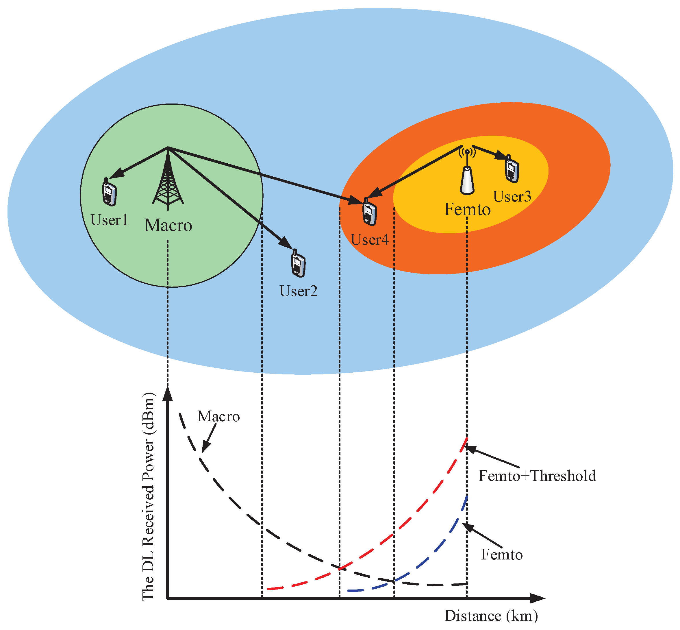
To elaborate, the proposed LA-CTC scheme is shown in Figure 1. User 1 located in the inner region of , and is only associated with . is close enough to guarantee the user 1’s quality of service (QoS). On the other hand, a user located in the outer region of will be associated with , or two tiers of BSs. User 2’s received power from is stronger than that from plus the cooperation threshold, and user 3’s received power from is stronger than that from ; thus user 2 and user 3 are only associated with and , respectively. Although user 4’s received power from is larger than that from , the received power from plus the cooperation threshold is larger. User 4 will be cooperatively served by and by means of jointly transmitting the user’s data; hence the user can be referred to as the CoMP user. Note that the prescribed value D is decided by the MBSs. In the current operation of cellular networks, a user will periodically feed back the measurement reports, including the user’s location information, to its serving BS for assisting the serving BS selection procedure [35]. Thus the MBSs classify the users as MIUs and MEUs through this procedure. Meanwhile, the FBSs use the pilot signals combined with a positive cooperation threshold to convince the vulnerable users to connect to both tiers of the BSs. The BSs use backhaul links (e.g., digital subscriber line (DSL)) [3,36] to exchange/share the users’ data and the control information, namely, the prescribed value D and the cooperation threshold. It is assumed that the users are stationary in this paper, that is, handoffs (HOs) do not occur for the BSs. This assumption is widely adopted in the extensive literature. When taking the mobility of users into account, the HO procedure will occur between different BSs such that different user association schemes are adopted. However, the high mobility users, such as users driving cars on the highways or taking high-speed trains, will have higher HO interruptions, which will degrade the network performance. To mitigate the HO effect, a location-aware HO skipping scheme for the macro tier can be adopted, which is similar to the scheme proposed in [37]. Additionally, our proposed LA-CTC scheme should be revised. In detail, it is assumed that the trajectory within the target MBS footprint is a priori via some trajectory estimation techniques [38,39]. Thus the HO skips associating to the target MBS if the user trajectory passes through the outer region of its target MBS; that is, when the minimum distance between the user trajectory and its target MBS exceeds the same predefined threshold value D, the HO occurs. However, the high-mobility users will skip HOs to the entire femto tier to avoid the excessive HOs because the FBS coverage area is too small [40]. The high-mobility users will be served directly by their un-skipped MBSs which are their trajectories pass through the inner region of the target MBSs.
We let , , and denote the probabilities that a typical user belongs to each of the above four disjoint user sets, respectively. Mathematically, this is , where . On the basis of the ergodicity of the PPP, these probabilities are derived in the following lemma.
Lemma 1.
, , and are given as follows:
If the path loss exponents are equal, that is, , , then can be reduced to a closed-form expression as:
where and .
Proof.
See Appendix A. ☐
2.3. The Signal-To-Interference-Plus-Noise Ratio for a Typical User
In the setup in Equation (1), given that the serving BS is located at , the received signal power for a typical user located at the origin, , can be expressed as:
where , and are Rayleigh-distributed random variables with average unit power, X and Y are the data sequences jointly transmitted by the serving and interfering BSs, respectively, and is a circular-symmetric zero-mean complex Gaussian random variable with variance to model the additive white Gaussian noise (AWGN) at the receiver. It is also assumed that no CSI (channel state information) is at the BSs. Hence, the received signal-to-interference-plus-noise ratio (SINR) of a typical user located at the origin, , is given by:
where is the indicator function that takes the value of 1 if the event A is true, and is the cumulative interference from the ith tier.
3. Analysis of the Coverage Probability and Average Rate
This section is the main technical component. On the basis of the characteristics of the SINR for the typical user, we derive the coverage probability and average rate of the typical user for the proposed LA-CTC scheme. We begin our discussion with the distance distributions to the serving BS for the typical user.
3.1. Statistical Distance to Serving Base Station
We denote , , and to be the distances between the typical user and their serving BSs.
Lemma 2.
The probability density functions (PDFs) of , , and are given as follows:
where
Proof.
See Appendix B. ☐
3.2. Coverage Probability
In the context of this paper, the coverage probability is formally defined as the probability that the typical user can achieve a target SINR threshold. Mathematically, this is , where is the target SINR threshold.
We denote , , and as the conditional coverage probabilities when a typical user belongs to one of the above four disjoint user sets, respectively. Following the law of total probability, the coverage probability of a randomly chosen user is
where , , and are given in Lemma 1.
Theorem 1.
Following the LA-CTC scheme in (1), the conditional coverage probabilities for the typical user are given by Equations (16)–(19).
where , and . The integral can be solved by the Gaussian hypergeometric function as [41]:
Proof.
See Appendix C. ☐
3.3. Average Rate
The average rate simply denotes the average number of nats transmitted per unit time per unit bandwidth (), which can represent the spectral efficiency of a user. Similarly to the conditional coverage probabilities defined in Theorem 1, the average rate for a typical user is given as:
where , , and are the average rates according to the proposed LA-CTC scheme above. The following theorem gives the average rate for a randomly chosen CoMP user. Note that the derivation of the average rate for other types of users can be obtained by following the same procedure, and hence it is skipped.
Theorem 2.
The average rate for a randomly chosen CoMP user is:
Proof.
The average rate for a randomly chosen CoMP user is formally defined as:
Because for , the can be rewritten as:
Using the definition of , we obtain the result in Equation (21). ☐
3.4. The Extension to the Multi-Tier Network
The performance analysis for our proposed scheme in the previous sections can be generalized to a network with more than two tiers. In the K-tier () setup, the small cells within the inner region of each MBS will all be deactivated. Similarly to Equations (1) and (2), a user can be divided into two disjoint sets for their serving tier :
Hence, the users in tier k can be classified into the non-CoMP users and the CoMP users . The set is the set of users in tier k, where . The non-CoMP users are directly served by the nearest BS in tier k, while the CoMP users are jointly served by the satisfactory BSs from two tiers. Together with the nearest BS in tier k, the offloaded BS from tier j () can cooperate to transmit the data for the offloaded users, in order to tackle the dominant interference from their original tier. More precisely, the cooperative BS set is defined as:
Lemma 3.
Let and denote the probabilities that a typical user belonging to tier k operates in the non-CoMP mode and in the CoMP mode, respectively. Then,
Proof.
See Appendix D. ☐
Lemma 4.
Let and denote the distances between the typical user and their serving BSs. Then, the PDFs of and are:
where , ,
and
Proof.
See Appendix E. ☐
Therefore, the coverage probability for a typical user can be derived by generalized forms, which are:
where ,
and
where the interference can be obtained from two parts: the tiers having a BS in cooperation to transmit the user’s data, and the tiers having no BS in cooperation. Then, we have the Laplace function of ():
where and , while the Laplace function of () is:
where and .
4. Numerical Results
In this section, we present the numerical results of the coverage probability and average rate for the proposed LA-CTC scheme, which can provide guidelines for the practical system design. Furthermore, we compare the proposed LA-CTC scheme with the other three user association schemes, which are the conventional MRP scheme [32], the CRE scheme [33] and the LA-CTCT scheme [23].
The transmit powers of MBSs and FBSs were dBm and dBm. The densities of the two tiers were and with . The user density was . The thermal noise power was assumed to be dBm (i.e., the system bandwidth was 10 MHz). For the evaluation of the coverage probability, τ was assumed to be 0 dB.
4.1. Validation of Analysis
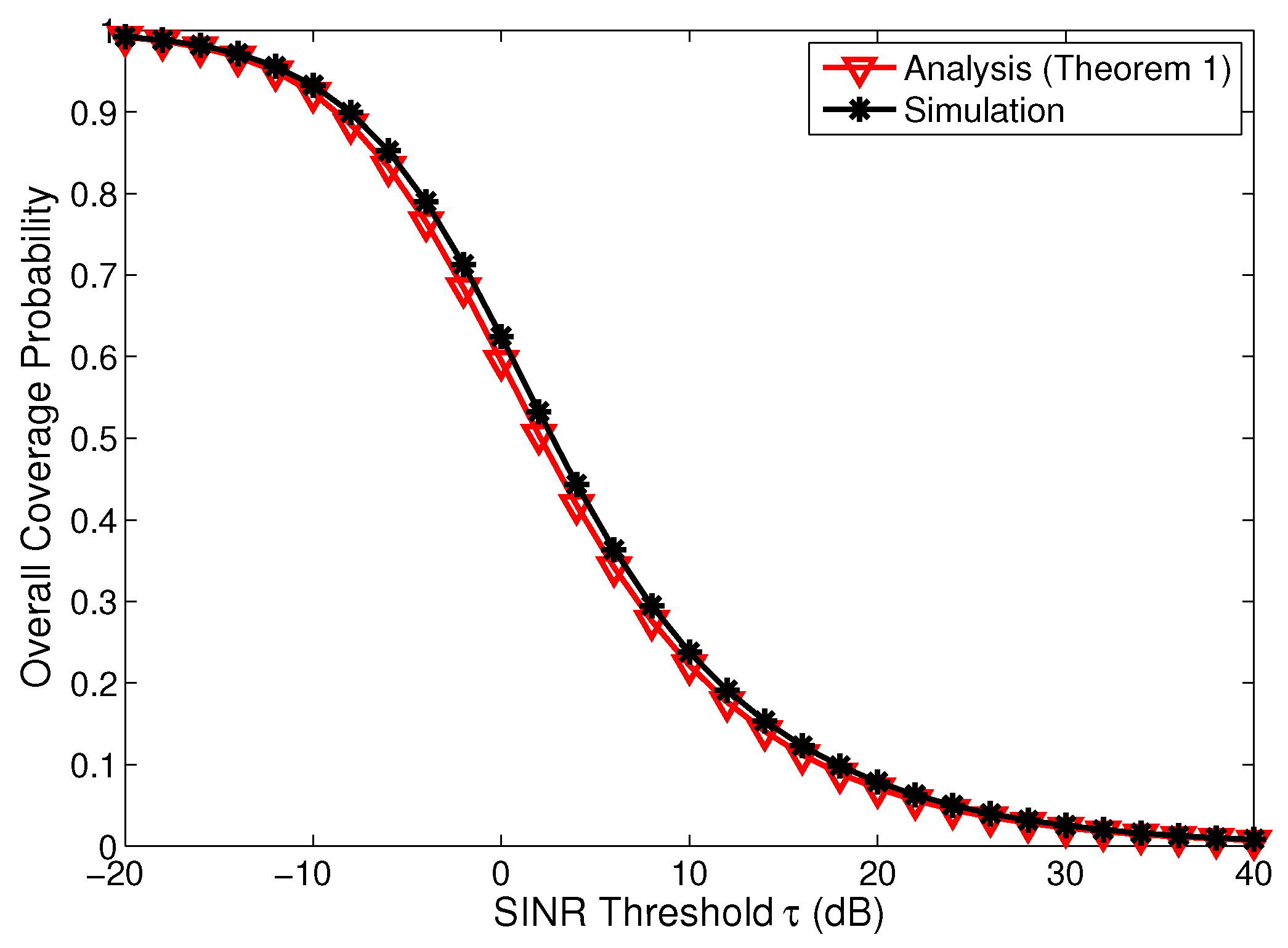
In Figure 2, the overall coverage probability for the LA-CTC scheme was validated by Monte Carlo simulations via MATLAB on a square window of 10 × 10 km. Each simulation result was averaged over iterations. For each realization, the locations of both the BSs and the users were generated by independent PPPs, while the FBSs within the inner region of each MBS were removed or deactivated. Then, the specific serving BS set was selected for each user on the basis of the LA-CTC scheme in Equation (1). The performance (i.e., coverage probability) of each user at each BS (which can be seen for a typical user at the origin) was evaluated. Finally, the mean value of the coverage probability was calculated. The details of the simulation procedure in [42] can be referred to as a pedagogical treatment to enable reproducibility. It can be seen that the analytical results match reasonably well with the simulation results. Hence, the performance trend of the LA-CTC scheme could be well captured by the analytical results. The small gaps were mainly due to the approximation of assuming that the density of the FBSs in the vicinity of the outer region was not changed.
4.2. Performance Evaluation: Trends and Discussion
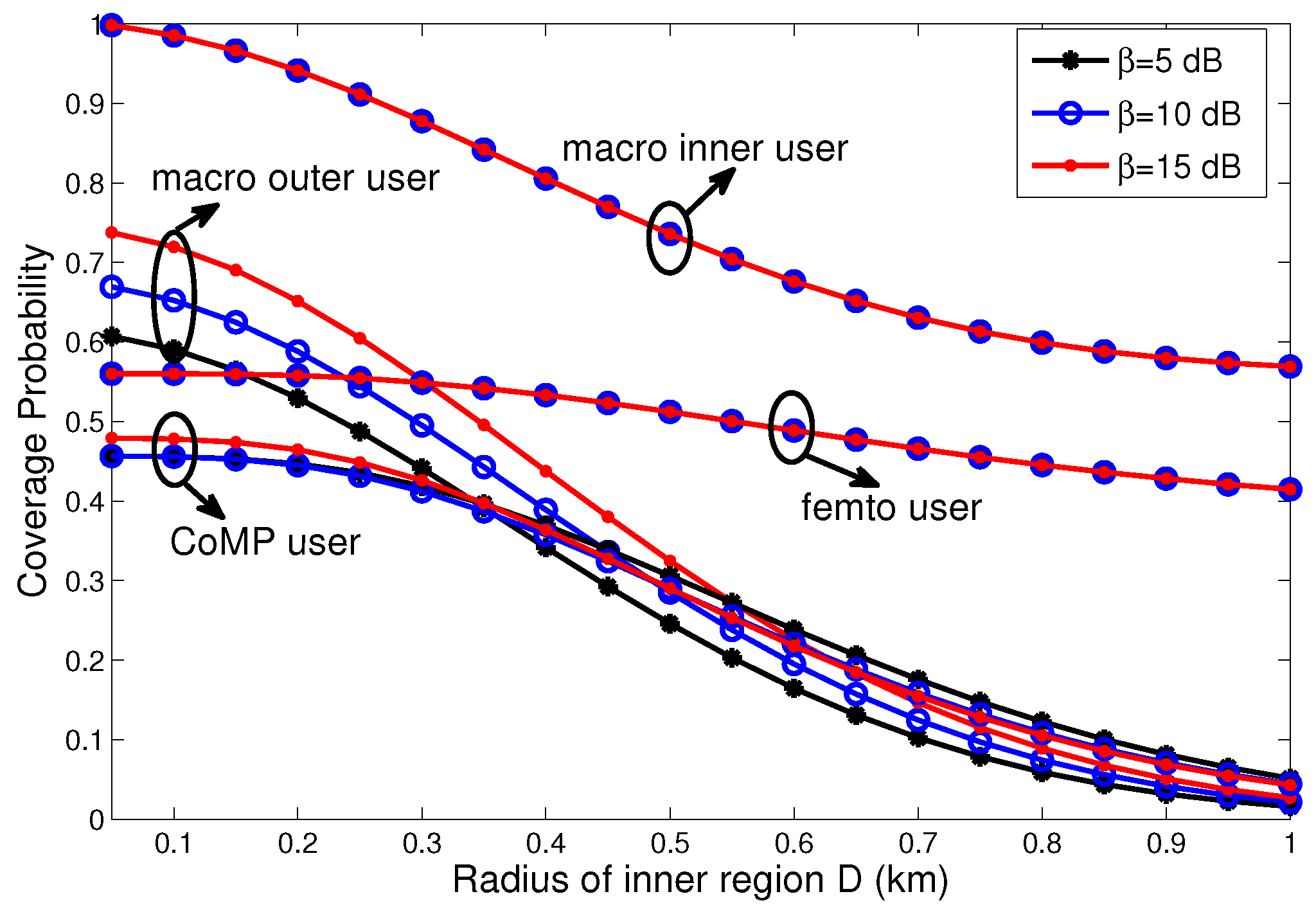
Before numerically analyzing the overall performance of the proposed scheme, we first analyze the conditional coverage probabilities of Equations (16)–(19) to obtain a better understanding of the overall performance trends. In Figure 3, it can be seen that the coverage probabilities of MIUs and femto users (i.e., and ) remained invariant with an increasing cooperation threshold, as and were independent of the cooperation threshold, whereas, as the radius of the inner region D increased, and decreased. This was because more macro users were allocated within the inner region; thus the interference from the macro tier increased. Meanwhile, the performance of femto users was degraded because more FBSs were deactivated. It can also be observed that the coverage probability of macro outer users (i.e., ) increased with an increasing cooperation threshold, as more users were offloaded to the femto tier. However, the coverage probability of the CoMP users (i.e., ) initially increased as the cooperation threshold increased, given an appropriate value of D, but it decreased beyond a certain prescribed distance value. This resulted from the fact that the non-uniform (cell-edge) deployment of FBSs can enhance the performance of CoMP users. When the prescribed distance exceeds a certain value, too many FBSs will be deactivated, which degrades the performance of CoMP users.
Figure 4 on the next page depicts the effect of increasing the radius of the inner region on the overall coverage probability and the average rate for different cooperation thresholds. It can be seen that the performance of the network can be improved by introducing the prescribed distance D (the radius of the inner region) for MBSs. The gains are obtained by the non-uniform deployment of FBSs. That is, the coverage area of FBSs increases and more users are offloaded to FBSs, as FBSs are deployed farther away from the MBSs. Hence, the more efficient deployment of FBSs enhances the performance of the network. For a given cooperation threshold, both the overall coverage probability and the average rate initially increase as the prescribed distance increases, but they decrease beyond a certain prescribed distance value. Hence, an optimal prescribed distance exists. The descending trend of the coverage probability and average rate is mainly due to more and more FBSs being deactivated, which degrades the network performance. This means that selecting an appropriate value of D indeed matters for the network performance.
The variation of the overall coverage probability and the average rate with an increasing cooperation threshold for different prescribed distances is also shown in Figure 4. It is clear that a higher coverage probability and average rate can be achieved by deploying the LA-CTC scheme, given an appropriate value of D. This improvement is due to the joint impact of offloading MEUs to FBSs and the CoMP transmission for the offloaded users. Therefore, the optimal network performance can be achieved by properly selecting the parameters of the LA-CTC scheme.
4.3. Performance Comparison with Other User Association Schemes
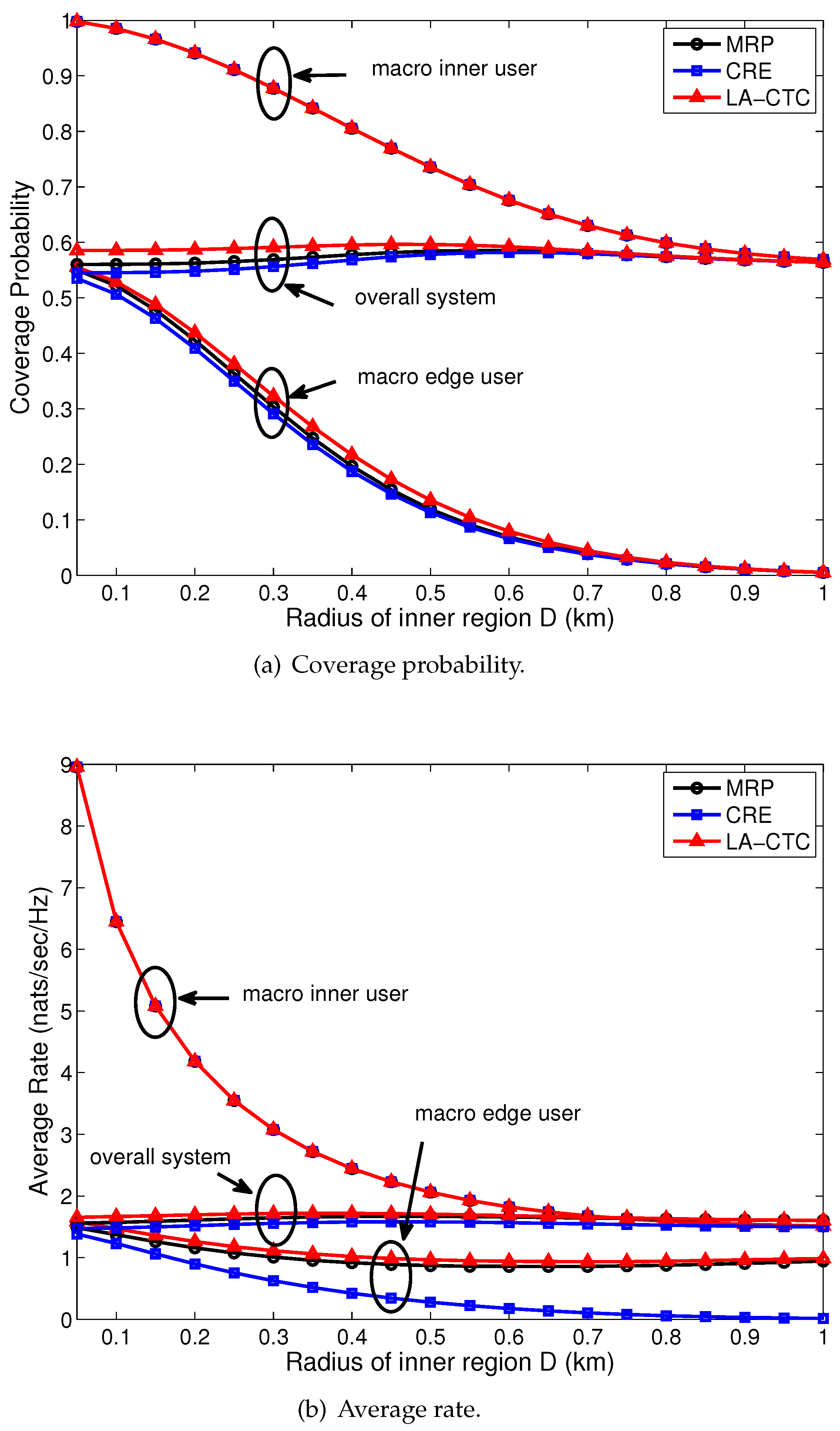
Figure 5 on the next page illustrates the coverage probability and average rate for the typical user with an increasing of the radius of the inner region D for the proposed LA-CTC scheme, for the MRP and for the CRE. From the perspective of MIUs, as the prescribed distance D increases, all schemes degrade the performance of the macro inner region while maintaining the same performance. This is caused by the fact that more users belong to the macro inner region; hence, the interference from the macro tier increases. In terms of the coverage and rate of the edge users and the overall system, the proposed LA-CTC scheme outperforms the MRP and the CRE. Compared to the MRP, the CRE degrades the performance of the macro edge region and the overall system. This is because the offloaded users usually do not experience the strongest received power, which deteriorates the SINR of the users. Note that all these results are obtained from the assumption that each BS has full buffer traffic downlink transmission for its connected user. On the other hand, compared to the CRE, the proposed LA-CTC scheme significantly improves the overall performance. This improvement is due to the offloaded users (i.e., CoMP users) being served by both the BSs, which improves the SINR of these users. The SINR degradation of offloaded users resulting from the CRE can be compensated for by CoMP transmission. Meanwhile, compared to the MRP, the overall performance gain from the proposed LA-CTC scheme results by means of jointly achieving load balancing for all the tiers and by interference mitigation for the offloaded users. The outperformance of the proposed LA-CTC scheme is guaranteed by the backhaul links between the BSs for exchanging the users’ data and the control information.
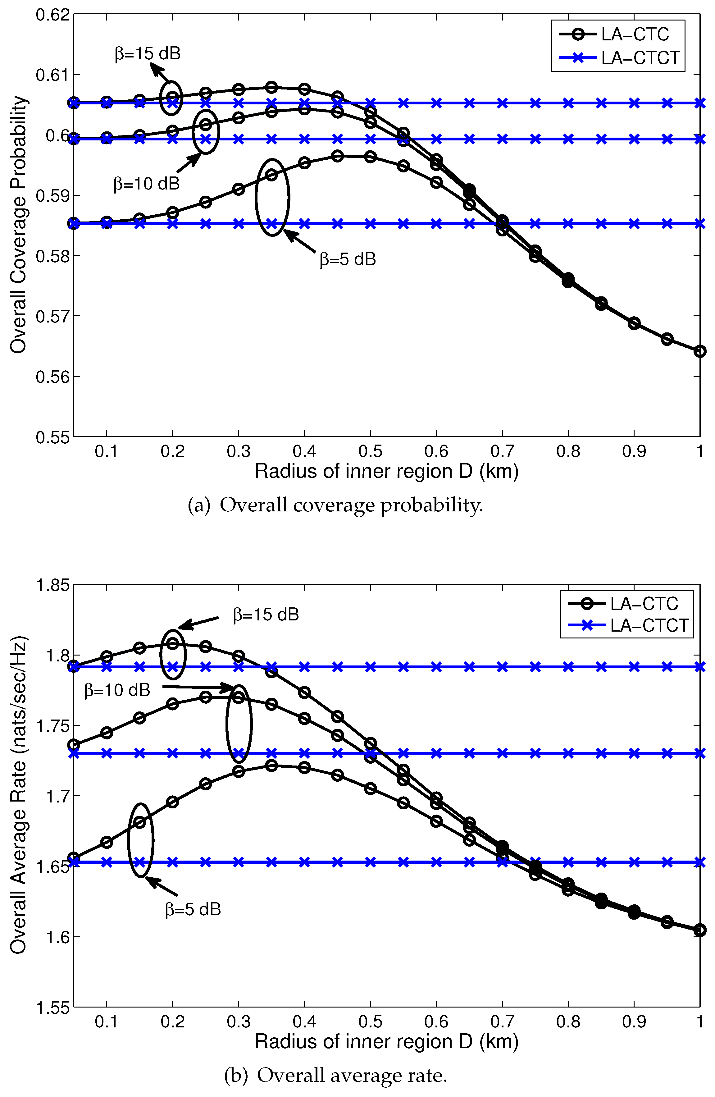
Figure 6 on the next page presents the overall coverage probability and the average rate versus the radius of the inner region D for the proposed LA-CTC scheme and for the LA-CTCT scheme [23]. The LA-CTCT scheme in [23] proposes cross-tier CoMP transmission for offloaded users when the small cells are uniformly deployed over the entire plane, without considering the poor offloading effect of small cells in the vicinity of the MBS. Therefore, by increasing the prescribed distance D, it can be seen in Figure 6 that the overall coverage probability and average rate of the LA-CTCT scheme remains invariant. However, the overall performance of the proposed LA-CTC scheme initially increases as the prescribed distance D increases, but decreases beyond a certain prescribed distance value. Compared to the LA-CTCT scheme, it is apparent that a higher overall coverage probability and average rate can be achieved by the proposed LA-CTC scheme, given an appropriate value of D. This improvement is due to the spatial separation between the MBSs and FBSs by means of deactivating the FBSs within the inner region of the MBSs. The excessive interference from the MBS to the FBS transmissions can be mitigated by this spatial separation.
5. Conclusions
In this paper, using tools of stochastic geometry, we presented an analytical framework to evaluate the coverage probability and the average rate for location-aware CoMP transmission in two-tier HetNets. A novel LA-CTC scheme was proposed and the mathematical coverage probability and average rate expressions were derived. The numerical results showed that the proposed LA-CTC scheme could improve the performance of a network significantly. In addition, the optimal network performance can be achieved by properly tuning the parameters of the proposed scheme. Moreover, the proposed scheme has been compared with the conventional MRP scheme, the CRE scheme and the LA-CTCT scheme, in terms of the coverage probability and the average rate. Numerical comparisons showed that the proposed LA-CTC scheme outperforms the other three schemes.
Acknowledgments
This paper was funded by the National Natural Science Foundation of China (Grant No. 61271263).
Author Contributions
Lili Guo and Shanya Cong conceived the proposed scheme. Lili Guo reviewed the manuscript. Shanya Cong conducted the detailed derivation to evaluate the performance of the proposed scheme and wrote the manuscript. All authors read and approved the final manuscript.
Conflicts of Interest
The authors declare no conflict of interest.
Appendix A
Following the PPP’s void probability [43], the probability a typical user u is located in the inner region can be calculated by:
When the typical user located in is also served by a MBS, the probability is hence derived as:
which: (a) follows the expectation of a measurable function of the random variable X, given by , given that X has a PDF of , and , which can be both obtained from [32], and (b) is obtained by approximating the density of FBSs in the vicinity of the outer region as [31,32,33]. In fact, the locations of FBSs originally drawn from a HPPP form a Poisson hole process (PHP) by the creation of exclusion zones around MBSs [43,44], which makes the characterization for the interference field and for the contact distance distribution of the PHP challenging. To maintain analytical tractability, it makes sense to ignore the effect of holes and to approximate the PHP by its original HPPP [31,32,33,44]. This is because of the fact that it is desirable to derive simple but tight approximations for obtaining useful system design insights. This approach leads to the lower but tight bound on the Laplace transform of the interference power [44].
Accordingly, the probability is similarly derived as:
Following from the law of total probability, the probability is eventually given by Equation (6).
Appendix B
Because the event is the event of on the condition that the typical user is served by the MBS, the probability of can be expressed as:
Then, the PDF of can be obtained by differentiating the foregoing expression.
Similarly, the cumulative distribution function (CDF) of is also given by:
The first term of the numerator in Equation (A1) can be derived as:
Substituting back into Equation (A1) and differentiating the resultant CDF, we have Equation (12).
Then, the CDF of is:
The first term of the numerator in Equation (A2) can be derived as:
Finally, the joint CDF of can be written as:
The first term of the numerator in Equation (A3) can be derived as:
Following the differentiation of Equation (A3), we obtain Equation (14), which completes the proof.
Appendix C
Firstly, we derive the coverage probability of a randomly chosen non-CoMP user, that is, . Using the definition of the coverage probability, then:
where is the range of the distance between the typical user and their serving BS, that is, , and .
Considering the definition of the Laplace transform, we have:
for which: (a) the above is obtained from the independence of , (b) it follows that , and (c) the above follows from the probability generating functional (PGFL) of and by replacing . Moreover, is the lower bound on the distance of the ith tier, which can be obtained by using Equation (2) as:
Using the change of variables with , the integral can be simplified to:
Hence, the Laplace transform of the interference is:
where .
For a randomly chosen CoMP user, that is, , the coverage probability is given by:
which is obtained from the independence assumption [19,23,31]:
where . Thus the received power from two cooperating BSs is approximated by the sum of two independent exponentially distributed random variables with mean because of the Rayleigh fading assumption and the independence of . This assumption gives a lower but tight bound on the Laplace transform of the interference power [19,23,31]. By following the same steps as for deriving Equation (A4), we obtain Equation (19) and complete the proof.
Appendix D
By the definition of association probability
and
The above two equations use the conditional PDFs of , which are:
The remaining derivation of and follows along the same lines as that of Lemma 1, and it is hence skipped.
Appendix E
The CDF of is:
The first term of the numerator in Equation (A5) can be derived as:
Substituting back into Equation (A5), the numerator in Equation (A5) can be derived as:
where
and .
Similarly to the derivation in Lemma 2, and are further given by:
where . Using the product rule for derivatives, the PDFs of and can be obtained by differentiating the foregoing expression.
References
- Andrews, J.G.; Buzzi, S.; Choi, W.; Stephen, V.H.; Lozano, A.; Soong Anthony, C.K.; Zhang, J.C. What will 5G be? IEEE J. Sel. Areas Commun. 2014, 32, 1065–1082. [Google Scholar] [CrossRef]
- Hossain, E.; Hasan, M. 5G cellular: Key enabling technologies and research challenges. IEEE Instrum. Meas. Mag. 2015, 18, 11–21. [Google Scholar] [CrossRef]
- Damnjanovic, A.; Montojo, J.; Wei, Y.; Ji, T.; Luo, T.; Vajapeyam, M.; Yoo, T.; Song, O.; Malladi, D. A survey on 3GPP heterogeneous networks. IEEE Wirel. Commun. 2011, 18, 11–21. [Google Scholar] [CrossRef]
- Liu, D.; Wang, L.; Chen, Y.; Elkashlan, M.; Wong, K.; Schober, R.; Hanzo, L. User association in 5G networks: A survey and an outlook. IEEE Commun. Surv. Tutor. 2016, 18, 1018–1044. [Google Scholar] [CrossRef]
- Kyocera. Potential performance of range expansion in macro-pico deployment (R1-104355). In Proceedings of the 3GPP TSG RAN WG1 Meeting-62, Madrid, Spain, 23–27 August 2010. [Google Scholar]
- Li, Q.; Hu, R.Q.; Qian, Y.; Wu, G. Cooperative communications for wireless networks: techniques and applications in LTE-advanced systems. IEEE Wirel. Commun. 2012, 19, 22–29. [Google Scholar]
- Gesbert, D.; Hanly, S.; Huang, H.; Shitz, S.S.; Simeone, O.; Yu, W. Multi-cell MIMO cooperative networks: A new look at interference. IEEE J. Sel. Areas Commun. 2010, 28, 1380–1408. [Google Scholar] [CrossRef]
- Irmer, R.; Droste, H.; Marsch, P.; Grieger, M.; Fettweis, G.; Brueck, S.; Mayer, H.P.; Thiele, L.; Jungnickel, V. Coordinated multipoint: Concepts, performance, and field trial results. IEEE Commun. Mag. 2011, 49, 102–111. [Google Scholar] [CrossRef]
- Lee, D.; Seo, H.; Clerckx, B.; Hardouin, E.; Mazzarese, D.; Nagata, S.; Sayana, K. Coordinated multipoint transmission and reception in LTE-advanced: Deployment scenarios and operational challenges. IEEE Commun. Mag. 2012, 50, 148–155. [Google Scholar] [CrossRef]
- Andrews, J.G.; Baccelli, F.; Ganti, R.K. A tractable approach to coverage and rate in cellular networks. IEEE Trans. Commun. 2011, 59, 3122–3134. [Google Scholar] [CrossRef]
- Dhillon, H.S.; Ganti, R.K.; Baccelli, F.; Andrews, J.G. Modeling and analysis of K-tier downlink heterogeneous cellular networks. IEEE J. Sel. Areas Commun. 2012, 30, 550–560. [Google Scholar] [CrossRef]
- Korrai, P.; Sen, D. Downlink SINR coverage and rate analysis with dual slope pathloss model in mmWave networks. In Proceedings of the 2017 IEEE Wireless Communications and Networking Conference (WCNC), San Francisco, CA, USA, 19–22 March 2017. [Google Scholar]
- Vien, Q.-T.; Akinbote, T.; Nguyen, H.X.; Trestian, R.; Gemikonakli, O. On the coverage and power allocation for downlink in heterogeneous wireless cellular networks. In Proceedings of the 2015 IEEE International Conference on Communications (ICC), London, UK, 8–12 June 2015. [Google Scholar]
- Jo, H.-S.; Sang, Y.J.; Xia, P.; Andrews, J.G. Heterogeneous cellular networks with flexible cell association: A comprehensive downlink SINR analysis. IEEE Trans. Wirel. Commun. 2012, 11, 3484–3495. [Google Scholar] [CrossRef]
- Singh, S.; Dhillon, H.S.; Andrews, J.G. Offloading in heterogeneous networks: Modeling, analysis, and design insights. IEEE Trans. Wirel. Commun. 2013, 12, 2484–2497. [Google Scholar] [CrossRef]
- Singh, S.; Zhang, X.; Andrews, J.G. Joint rate and SINR coverage analysis for decoupled uplink-downlink biased cell associations in hetNets. IEEE Trans. Wirel. Commun. 2015, 14, 5360–5373. [Google Scholar] [CrossRef]
- Novlan, T.D.; Ganti, R.k.; Ghosh, A.; Andrews, J.G. Analytical evaluation of fractional frequency reuse for OFDMA cellular networks. IEEE Trans. Wirel. Commun. 2011, 10, 4294–4305. [Google Scholar] [CrossRef]
- Novlan, T.D.; Ganti, R.K.; Ghosh, A.; Andrews, J.G. Analytical evaluation of fractional frequency reuse for heterogeneous cellular networks. IEEE Trans. Commun. 2012, 60, 2029–2039. [Google Scholar] [CrossRef]
- Nigam, G.; Minero, P.; Haenggi, M. Coordinated multipoint joint transmission in heterogeneous networks. IEEE Trans. Commun. 2014, 62, 4134–4146. [Google Scholar] [CrossRef]
- Xia, P.; Liu, C.-H.; Andrews, J.G. Downlink coordinated multipoint with overhead modeling in heterogeneous cellular networks. IEEE Trans. Wirel. Commun. 2013, 12, 4025–4037. [Google Scholar] [CrossRef]
- Baccelli, F.; Giovanidis, A. A stochastic geometry framework for analyzing pairwise-cooperative cellular networks. IEEE Trans. Wirel. Commun. 2015, 14, 794–808. [Google Scholar] [CrossRef]
- Tanbourgi, R.; Singh, S.; Andrews, J.G.; Jondral, F.K. A tractable model for non-coherent joint-transmission base station cooperation. IEEE Trans. Wirel. Commun. 2014, 13, 4959–4973. [Google Scholar] [CrossRef]
- Sakr, A.H.; Hossain, E. Location-aware cross-tier coordinated multipoint transmission in two-tier cellular networks. IEEE Trans. Wirel. Commun. 2014, 13, 6311–6325. [Google Scholar] [CrossRef]
- Lopez-Perez, D.; Guvenc, I.; De La Roche, G.; Kountouris, M.; Quek, T.Q.; Zhang, J. Enhanced intercell interference coordination challenges in heterogeneous networks. IEEE Wirel. Commun. 2011, 18, 22–31. [Google Scholar] [CrossRef]
- Singh, S.; Andrews, J.G. Joint resource partitioning and offloading in heterogeneous cellular networks. IEEE Trans. Wirel. Commun. 2014, 13, 888–901. [Google Scholar] [CrossRef]
- Dhungana, Y.; Tellambura, C. Multichannel analysis of cell range expansion and resource partitioning in two-tier heterogeneous cellular networks. IEEE Trans. Wirel. Commun. 2016, 15, 2394–2406. [Google Scholar] [CrossRef]
- Xie, B.; Zhang, Z.; Hu, R.Q.; Qian, Y. Spectral efficiency analysis in wireless heterogeneous networks. In Proceedings of the 2016 IEEE International Conference on Communications (ICC), Kuala Lumpur, Malaysia, 22–27 May 2016. [Google Scholar]
- Merwaday, A.; Mukherjee, S.; Guvenc, I. Capacity analysis of LTE-advanced HetNets with reduced power subframes and range expansion. EURASIP J. Wirel. Commun. Netw. 2014, 2014, 189. [Google Scholar] [CrossRef]
- Khoriaty, J.; Artail, H. Coordinated multipoint in heterogeneous networks with overlapping microcell expanded regions. In Proceedings of the 2015 IEEE 11th International Conference on Wireless and Mobile Computing, Networking and Communications (WiMob), Abu Dhabi, UAE, 19–21 Octomber 2015. [Google Scholar]
- Yang, K.; Zhang, J.; Zhang, X.; Wang, W. Edge aware cross-tier base station cooperation in heterogeneous wireless networks with non-uniformly-distributed nodes. IET Commun. 2016, 10, 1896–1903. [Google Scholar] [CrossRef]
- Wu, H.; Tao, X.; Xu, J.; Li, N. Coverage analysis for CoMP in two-tier HetNets with non-uniformly deployed femtocells. IEEE Commun. Lett. 2015, 19, 1600–1603. [Google Scholar] [CrossRef]
- Wang, H.; Zhou, X.; Reed, M.C. Coverage and throughput analysis with a non-uniform small cell deployment. IEEE Trans. Wirel. Commun. 2014, 13, 2047–2059. [Google Scholar] [CrossRef]
- Muhammad, F.; Abbas, Z.H.; Li, F.Y. Cell association with load balancing in non-uniform heterogeneous cellular networks: coverage probability and rate analysis. IEEE Trans. Veh. Technol. 2016, 99, 1–15. [Google Scholar]
- Muhammad, M.P.; Abbas, Z.H.; Muhammad, F.; Jiao, L. Location-based coverage and capacity analysis of a two tier HetNet. IET Commun. 2017, 11, 1067–1073. [Google Scholar]
- Dahlman, E.; Parkvall, S.; Skold, J.; Beming, P. 3G Evolution: HSPA and LTE for Mobile Broadband, 2nd ed.; Elsevier: Amsterdam, The Netherlands, 2008. [Google Scholar]
- Pantisano, P.; Bennis, M.; Saad, W.; Debbah, M.; Latva-aho, M. On the impact of heterogeneous backhauls on coordinated multipoint transmission in femtocell networks. In Proceedings of the 2012 IEEE International Conference on Communications (ICC), Ottawa, ON, Canada, 10–15 June 2012. [Google Scholar]
- Arshad, R.; Elsawy, H.; Sorour, S.; Y.Al-Naffouri, T.; Alouini, M.-S. Handover management in 5G and beyond: A topology aware skipping approach. IEEE Access. 2016, 4, 9073–9081. [Google Scholar] [CrossRef]
- Milocco, H.R.; Boumerdassi, S. Estimation and prediction for tracking trajectories in cellular networks using the recursive prediction error method. In Proceedings of the 2010 IEEE International Symposium on a World of Wireless Mobile and Multimedia Networks (WoWMoM), Montrreal, QC, Canada, 14–17 June 2010. [Google Scholar]
- Leontiadis, I.; Lima, A.; Kwak, H.; Stanojevic, R.; Wetherall, D.; Papagiannaki, K. From cells to streets: Estimating mobile paths with cellular-side data. In Proceedings of the The 10th ACM International on Conference on emerging Networking Experiments and Technologies, Sydney, Australia, 2–5 December 2014. [Google Scholar]
- Arshad, R.; Elsawy, H.; Sorour, S.; Y.Al-Naffouri, T.; Alouini, M.-S. Velocity-aware handover management in two-tier cellular networks. IEEE Trans. Wirel. Commun. 2017, 16, 1851–1867. [Google Scholar] [CrossRef]
- Mukherjee, S. Distribution of downlink SINR in heterogeneous cellular networks. IEEE J. Sel. Areas Commun. 2012, 30, 54–64. [Google Scholar] [CrossRef]
- Merwaday, A.; Mukherjee, S.; Guvenc, I. On the capacity analysis of HetNets with range expansion and eICIC. In Proceedings of the 2013 IEEE Global Communications Conference (GLOBECOM), Atlanta, GA, USA, 9–13 December 2013. [Google Scholar]
- Haenggi, M. Stochastic Geometry for Wireless Networks; Cambridge University Press: New York, NY, USA, 2012. [Google Scholar]
- Lee, C.-H.; Haenggi, M. Interference and outage in Poisson cognitive networks. IEEE Trans. Wirel. Commun. 2012, 11, 1392–1401. [Google Scholar] [CrossRef]
Figure 1.
Illustration of the proposed location-aware cross-tier cooperation (LA-CTC) scheme.

Figure 2.
Validation of the analytical results for the overall coverage probability via Monte Carlo simulations with D = 0.5 km and dB.
Figure 2.
Validation of the analytical results for the overall coverage probability via Monte Carlo simulations with D = 0.5 km and dB.

Figure 3.
Effect of the radius of the inner region on the conditional coverage probabilities of four types of users for different cooperation thresholds.
Figure 3.
Effect of the radius of the inner region on the conditional coverage probabilities of four types of users for different cooperation thresholds.

Figure 4.
Effect of the radius of inner region on the overall coverage probability and average rate for different cooperation thresholds. (a) Overall coverage probability; (b) Overall average probability.
Figure 4.
Effect of the radius of inner region on the overall coverage probability and average rate for different cooperation thresholds. (a) Overall coverage probability; (b) Overall average probability.
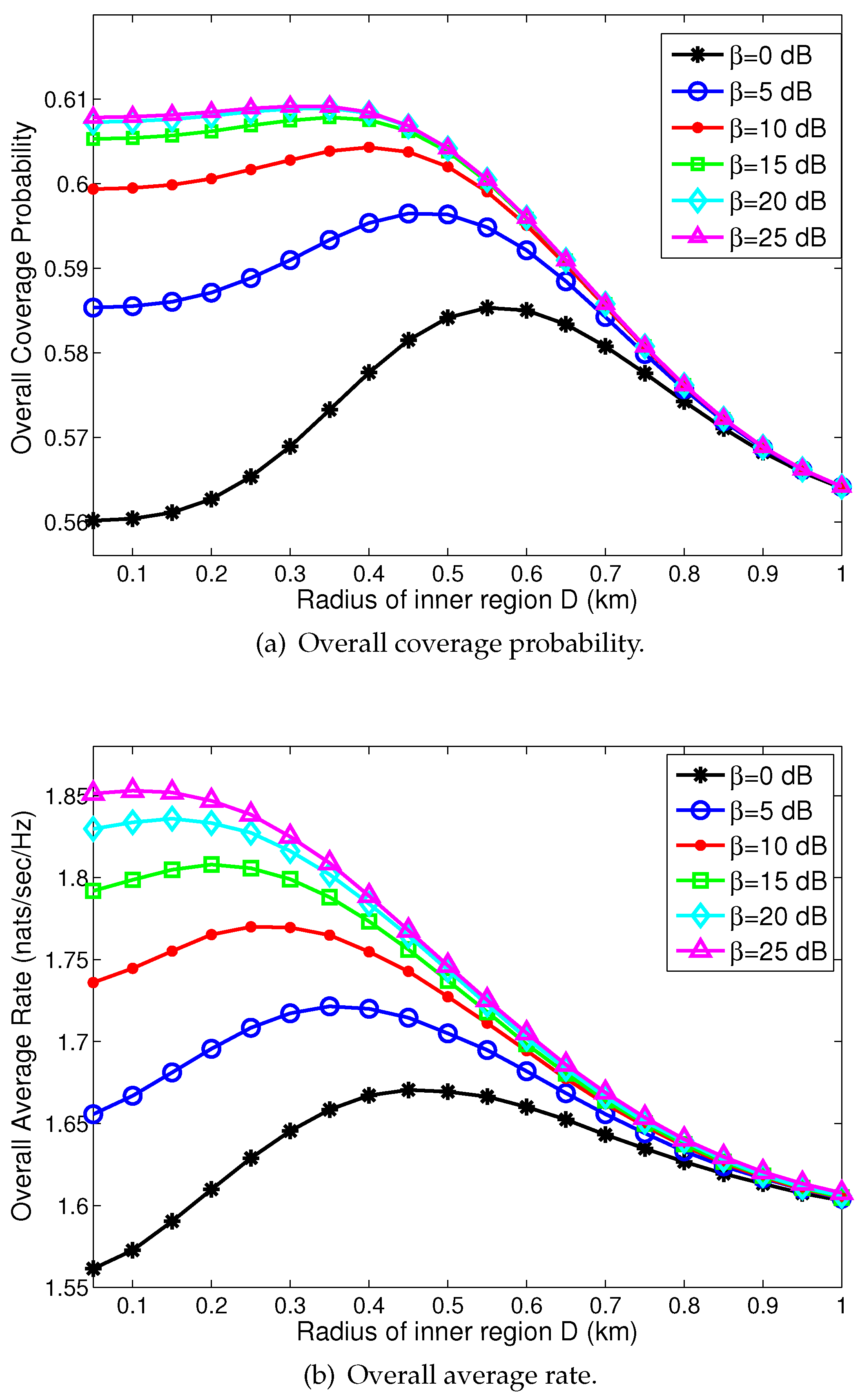
Figure 5.
The coverage probability and average rate for the proposed location-aware cross-tier cooperation (LA-CTC) scheme, the maximum-received-power (MRP) and the cell range expansion (CRE) when the cooperation threshold (bias factor) β = 5 dB. (a) Coverage probability; (b) Average rate.
Figure 5.
The coverage probability and average rate for the proposed location-aware cross-tier cooperation (LA-CTC) scheme, the maximum-received-power (MRP) and the cell range expansion (CRE) when the cooperation threshold (bias factor) β = 5 dB. (a) Coverage probability; (b) Average rate.

Figure 6.
The overall coverage probability and average rate for the proposed location-aware cross-tier cooperation (LA-CTC) scheme and location-aware cross-tier CoMP transmission (LA-CTCT) scheme with different cooperation thresholds. (a) Overall coverage probability; (b) Overall average rate.
Figure 6.
The overall coverage probability and average rate for the proposed location-aware cross-tier cooperation (LA-CTC) scheme and location-aware cross-tier CoMP transmission (LA-CTCT) scheme with different cooperation thresholds. (a) Overall coverage probability; (b) Overall average rate.

© 2017 by the authors. Licensee MDPI, Basel, Switzerland. This article is an open access article distributed under the terms and conditions of the Creative Commons Attribution (CC BY) license (http://creativecommons.org/licenses/by/4.0/).
Share and Cite
MDPI and ACS Style
Guo, L.; Cong, S. Coverage and Rate Analysis for Location-Aware Cross-Tier Cooperation in Two-Tier HetNets. Symmetry 2017, 9, 157. https://doi.org/10.3390/sym9080157
AMA Style
Guo L, Cong S. Coverage and Rate Analysis for Location-Aware Cross-Tier Cooperation in Two-Tier HetNets. Symmetry. 2017; 9(8):157. https://doi.org/10.3390/sym9080157
Chicago/Turabian StyleGuo, Lili, and Shanya Cong. 2017. "Coverage and Rate Analysis for Location-Aware Cross-Tier Cooperation in Two-Tier HetNets" Symmetry 9, no. 8: 157. https://doi.org/10.3390/sym9080157
Note that from the first issue of 2016, this journal uses article numbers instead of page numbers. See further details here.