The Orthogonality between Complex Fuzzy Sets and Its Application to Signal Detection

Abstract

A complex fuzzy set is a set whose membership values are vectors in the unit circle in the complex plane. This paper establishes the orthogonality relation of complex fuzzy sets. Two complex fuzzy sets are said to be orthogonal if their membership vectors are perpendicular. We present the basic properties of orthogonality of complex fuzzy sets and various results on orthogonality with respect to complex fuzzy complement, complex fuzzy union, complex fuzzy intersection, and complex fuzzy inference methods. Finally, an example application of signal detection demonstrates the utility of the orthogonality of complex fuzzy sets.

1. Introduction

Complex fuzzy sets [1] are an important extension of fuzzy set theory. In recent years, complex fuzzy sets have been successfully used in complex fuzzy inference systems for various applications, such as time series prediction [2,3,4,5,6,7,8], function approximation [9,10,11], and image restoration [12,13]. A complex fuzzy set A on a universe of discourse U is a mapping from U to the unit disc in the complex plane. Thus a complex fuzzy set is a set of vectors in the complex plane. This idea of membership vectors greatly inspired how definition of complex fuzzy sets operations [14,15] and complex fuzzy logic systems [16,17,18,19,20,21] and how to measures the difference between two complex fuzzy sets [22,23,24].

Orthogonality is an important concept in mathematics and computer science. For instance, orthogonality in geometry means that two vectors are perpendicular. Orthogonality in programming language design is the ability to use different language features in different combinations with consistent results [25]. Then, a question arises: why do we need to study the orthogonality between complex fuzzy sets?

The literature review shows two main reasons for studying the orthogonality between complex fuzzy sets. (1) Orthogonality is also an important tool in traditional fuzzy systems. Orthogonal transformation method, orthogonal rule, and orthogonal approximation concept are frequently applied to fuzzy rule-based models [26,27,28], fuzzy neural networks [29,30], and fuzzy control [31,32]. Complex fuzzy sets as an extension of fuzzy sets have been studied. When we apply these orthogonal methods to complex fuzzy systems, the concept of orthogonality should be considered. (2) Recently, complex fuzzy sets have been used in image restoration [12,13] and signal processing [1,23]. In these applications, various orthogonal data, such as orthogonal signals and orthogonal images, are often considered. So, the concept of orthogonality also should be considered when we apply complex fuzzy sets to these applications.

Our goal in this paper is to present the concept and properties of orthogonality for complex fuzzy sets. In our view, this is analogous to orthonormal vectors. As mentioned in [16], the membership function of a complex fuzzy set can be viewed as a vector in the complex plane. As is well known, a vector has length and direction. There are various properties concerning the direction of vectors. The orthogonality relation is an important concept in vector theory when a complex fuzzy set is viewed as a set of vectors and a complex fuzzy logic is viewed as a logic of vectors. We should consider the direction properties for complex fuzzy sets and complex fuzzy logic. Having this in mind, we propose the orthogonality for complex fuzzy sets. Then, their implications for the possible choices of complex fuzzy operations are examined. The representation of complex fuzzy set S is given by $r_A\left(x\right)·e^{j{w}_A\left(x\right)}$, the amplitude term $r_A\left(x\right)$ and the phase term $w_A\left(x\right)$ are both real-valued, $r_A\left(x\right)\in [0,1]$, and $j=\sqrt{-1}$. We also can use the form $r_A\left(x\right)\cos \left(w_A\left(x\right)\right)+j{r}_A\left(x\right)\sin \left(w_A\left(x\right)\right)$. This form is based on two orthonormal vectors, $(1,0)$ and $(0,1)$, corresponding to the complex numbers $1+j0$ and $0+j$, respectively. These two vectors are the most used orthonormal basis in complex plane. The concept of orthogonality has been used in complex fuzzy sets naturally, but it has not formed systemic cognition and there has been a lack of standardized study.

The main contribution of the study includes. (1) A concept of orthogonality for complex fuzzy sets; (2) An idea for the possible choices of complex fuzzy operators: a complex fuzzy operation should preserve the orthogonality. In the practical application of complex fuzzy sets, one of the key research issues is how to select a suitable complex fuzzy operation. We investigate this idea in depth, and then examine its implications for the possible choices of complex fuzzy inference; and (3) A signal detection method which involves the orthogonality complex fuzzy sets. Operations used in this method have the orthogonality preserving property.

The remainder of this paper is organized in the following way. In Section 2, the concept of orthogonality of complex fuzzy sets is introduced, and their properties investigated. In Section 3, we discuss whether orthogonality can be preserved for complex fuzzy complement, complex fuzzy union, complex fuzzy intersection and complex fuzzy inference system, and present an application example in signal detection. Discussion and conclusion are presented in Section 4.

2. Materials and Methods

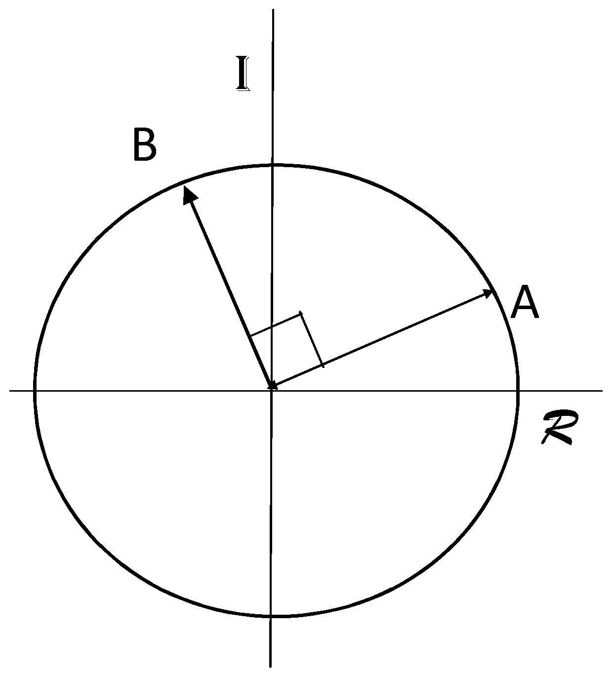
In this section we introduce the concept of orthogonality of complex fuzzy sets, which should be contrasted with the concept of orthogonality in mathematics such as $x\perp y$ between two vectors x and y. By intuition, this is analogous to the orthogonality of vectors, orthogonality is the relation of two complex fuzzy sets where the angle between membership vectors of each element of the universal set are perpendicular. As shown in Figure 1 , two membership vectors A and B of an element of U are orthogonality (perpendicular).

A complex fuzzy set A, defined on a universe of discourse U, is characterized by a membership function ${\mu }_A\left(x\right)$ that assigns any element $x\in U$ a complex-valued grade of membership in A.

Let $F^C\left(U\right)$ be the set of all complex fuzzy sets on U. The complex fuzzy set A may be represented as the set of ordered pairs:

$$A=\left\{(x,{\mu }_A\left(x\right))\right|x\in U\}$$

(1)

where the membership function ${\mu }_A\left(x\right)$ is of the form $r_A\left(x\right)·e^{j{w}_A\left(x\right)}$, $j=\sqrt{-1}$, the amplitude term $r_A\left(x\right)$ and the phase term $w_A\left(x\right)$ are both real-valued, and $r_A\left(x\right)\in [0,1]$.

The inner product $<{\mu }_A\left(x\right),{\mu }_B\left(x\right)>$ of membership vectors of $x\in U$ is defined as:

$$<{\mu }_A\left(x\right),{\mu }_B\left(x\right)>=r_A\left(x\right)·r_B\left(x\right)·\cos \left(\right|w_A\left(x\right)-w_B\left(x\right)\left|\right)$$

(2)

Definition 1.

Let A and B be two complex fuzzy sets on U, and ${\mu }_A\left(x\right)=r_A\left(x\right)·e^{j{w}_A\left(x\right)}$ and ${\mu }_B\left(x\right)=r_B\left(x\right)·e^{j{w}_B\left(x\right)}$ their membership functions, respectively. A and B are said to be orthogonal if $<{\mu }_A\left(x\right),{\mu }_B\left(x\right)>=0$ for each $x\in U$ and it is denoted by $A\perp B$. Similarly, for the subsets $\mathcal{C},\mathcal{D}\subseteq F^C\left(U\right)$, we write $A\perp \mathcal{C}$ if $A\perp \mathcal{C}$ for all $C\in \mathcal{C}$ and $\mathcal{C}\perp \mathcal{D}$ if $C\perp D$ for all $C\in \mathcal{C}$ and all $D\in \mathcal{D}$.

Theorem 1.

The orthogonality of complex fuzzy sets has the following properties:

(i) 

0 $\perp A$ for all $A\in F^C\left(U\right)$,

(ii) 

if $A\perp B$ then $B\perp A$,

(iii) 

if $A\perp A$ then $A=$ 0.

Proof. 

Trivial. ☐

The proof is simple and we omit the details. In this paper, we omit proofs of some results which can be easily obtained.

Remark 1.

0 denote the complex fuzzy set where the membership vectors of each element of the universal set is the zero vector.

In practice, orthogonality may be represented as independent or uncorrelated objects. The orthogonality between complex fuzzy sets may be seen as a theory or method for handling the relativity and dependence among complex data. The following problems are interesting.

Problem 1.

Suppose $A\perp B$ and $A\perp C$, then whether or not $A\perp (B\circ C)$, where $\circ$ is some operation of complex fuzzy sets.

Problem 2.

Suppose $A\perp B$, then whether or not $f\left(A\right)\perp f\left(B\right)$, where f is some complex fuzzy inference method.

3. Results

In this section, we discuss whether orthogonality can be preserved for complex fuzzy complement, complex fuzzy union, and complex fuzzy intersection, i.e., Problems 1 and 2.

The concept of orthogonality preserving is formally expressed as follows.

Definition 2.

Let $f:F^C\left(U\right)\to F^C\left(U\right)$ be a function, f is orthogonality preserving if:

$$A\perp B\Rightarrow f\left(A\right)\perp f\left(B\right)$$

(3)

for any $A,B\in F^C\left(U\right)$.

Obviously, set rotation and reflection operations, described in [1], are orthogonality preserving.

Let A be a complex fuzzy set on U and ${\mu }_A\left(x\right)=r_A\left(x\right)·e^{j{w}_A\left(x\right)}$ its membership functions. The rotation of A by $\theta$ radians, denoted $Ro{t}_{\theta }\left(A\right)$ is defined as:

$$Ro{t}_{\theta }\left({\mu }_A\left(x\right)\right)=r_A\left(x\right)·e^{j(w_A\left(x\right)+\theta )}$$

(4)

The reflection of A , denoted $Ref\left(A\right)$ is defined as:

$$Ref\left({\mu }_A\left(x\right)\right)=r_A\left(x\right)·e^{-j{w}_A\left(x\right)}$$

(5)

Theorem 2.

Let A and B be two complex fuzzy sets on U.

(i) 

If $A\perp B$ then $Ref\left(A\right)\perp Ref\left(B\right)$.

(ii) 

If $A\perp B$ then $Ro{t}_{\theta }\left(A\right)\perp Ro{t}_{\theta }\left(B\right)$ for any θ radians.

Proof. 

Trivial. ☐

3.1. Complex Fuzzy Complement

The complement of a complex fuzzy set is an extension of the definition of the traditional fuzzy complement. Ramot et al. [1] introduced the following three complex fuzzy complements.

Let A be a complex fuzzy set on U and ${\mu }_A\left(x\right)=r_A\left(x\right)·e^{j{w}_A\left(x\right)}$ its membership functions. The complex fuzzy complement of A, denoted $\neg A$ is specified by a function:

$$\begin{array}{cc}\hfill {\mu }_{{\neg }_{1}A}\left(x\right)& =c\left(r_A\left(x\right)\right)·e^{j(-w_A\left(x\right))}\hfill \end{array}$$

(6)

$$\begin{array}{cc}\hfill {\mu }_{{\neg }_{2}A}\left(x\right)& =c\left(r_A\left(x\right)\right)·e^{j\left(w_A\left(x\right)\right)}\hfill \end{array}$$

(7)

$$\begin{array}{cc}\hfill {\mu }_{{\neg }_{3}A}\left(x\right)& =c\left(r_A\left(x\right)\right)·e^{j(w_A\left(x\right)+\pi )}\hfill \end{array}$$

(8)

where $c\left(r_A\left(x\right)\right)=1-r_A\left(x\right)$.

Theorem 3.

Let A and B be two complex fuzzy sets on U and ${\mu }_A\left(x\right)=r_A\left(x\right)·e^{j{w}_A\left(x\right)}$ and ${\mu }_B\left(x\right)=r_B\left(x\right)·e^{j{w}_B\left(x\right)}$ their membership functions, respectively. Support ${\mu }_A\left(x\right)\ne 0$ and ${\mu }_B\left(x\right)\ne 0$ for all $x\in U$. If $A\perp B$, then ${\neg }_{i}A\perp {\neg }_{i}B$, $i\in \{1,2,3\}$.

Proof. 

We only consider the case of $i=1$. For any $x\in U$, by $A\perp B$, we have:

$$<{\mu }_A(x,{\mu }_B\left(x\right))>=r_A\left(x\right)·r_B\left(x\right)·\cos \left(\right|w_A\left(x\right)-w_B\left(x\right)\left|\right)=0$$

Because ${\mu }_A\left(x\right)\ne 0$ and ${\mu }_B\left(x\right)\ne 0$, thus:

$$\cos \left(\right|w_A\left(x\right)-w_B\left(x\right)\left|\right)=0$$

By the definition of the complex fuzzy complement:

$${\mu }_{\neg A}\left(x\right)=(1-r_A\left(x\right))·e^{j(-w_A\left(x\right))},$$

$${\mu }_{\neg B}\left(x\right)=(1-r_B\left(x\right))·e^{j(-w_B\left(x\right))},$$

We obtain:

$$\begin{array}{cc}<{\mu }_{{\neg }_{1}A}\left(x\right),{\mu }_{{\neg }_{1}B}\left(x\right)>& =c\left(r_A\left(x\right)\right)·c\left(r_B\left(x\right)\right)·\cos \left(\right|-w_A\left(x\right)+w_B\left(x\right)\left|\right)\hfill \\ & =c\left(r_A\left(x\right)\right)·c\left(r_B\left(x\right)\right)·\cos \left(\right|w_A\left(x\right)-w_B\left(x\right)\left|\right)\hfill \\ & =0.\hfill \end{array}$$

Thus ${\neg }_{1}A\perp {\neg }_{1}B$ ☐

Example 1.

Assume two complex fuzzy sets A and B are given by:

$$\begin{array}{cc}\hfill A=& 0.1e^{j1.5\pi }/x_1+0.2e^{j0.3\pi }/x_2\hfill \\ \hfill B=& 0.2e^{j\pi }/x_1+0.4e^{j0.8\pi }/x_2\hfill \end{array}$$

We see $A\perp B$. Then we have:

$$\begin{array}{cc}\hfill {\neg }_{1}A=& 0.9e^{j0.5\pi }/x_1+0.8e^{j1.7\pi }/x_2\hfill \\ \hfill {\neg }_{1}B=& 0.8e^{j\pi }/x_1+0.6e^{j1.2\pi }/x_2\hfill \\ \hfill {\neg }_{2}A=& 0.9e^{j1.5\pi }/x_1+0.8e^{j0.3\pi }/x_2\hfill \\ \hfill {\neg }_{2}B=& 0.8e^{j\pi }/x_1+0.6e^{j0.8\pi }/x_2\hfill \\ \hfill {\neg }_{3}A=& 0.9e^{j0.5\pi }/x_1+0.8e^{j1.3\pi }/x_2\hfill \\ \hfill {\neg }_{3}B=& 0.8e^{j2\pi }/x_1+0.6e^{j1.8\pi }/x_2.\hfill \end{array}$$

It is easy to verify ${\neg }_{i}A\perp {\neg }_{i}B$ for any $i\in \{1,2,3\}$

3.2. Complex Fuzzy Union

The complex fuzzy union of complex fuzzy sets are reviewed as follows (see [1]).

Let A and B be two complex fuzzy sets on U and ${\mu }_A\left(x\right)=r_A\left(x\right)·e^{j{w}_A\left(x\right)}$ and ${\mu }_B\left(x\right)=r_B\left(x\right)·e^{j{w}_B\left(x\right)}$ their membership functions, respectively. The complex fuzzy union of A and B, denoted $A\cup B$, is specified by a function:

$${\mu }_{A\cup B}\left(x\right)=(r_A\left(x\right)\oplus r_B\left(x\right))·e^{j{w}_{A\otimes B}\left(x\right)}$$

(9)

where ⊕ represents a t-conorm function.

The functions given below are possibilities for calculating $w_{A\otimes B}$:

$$\begin{array}{cccc}\hfill & \mathrm{Sum}:\hfill & \hfill w_{A\otimes B}& =w_A+w_B\hfill \end{array}$$

(10)

$$\begin{array}{cccc}\hfill & \mathrm{Max}:\hfill & \hfill {\mu }_{A\cup B}& =\max (w_A,w_B)\hfill \end{array}$$

(11)

$$\begin{array}{ccc}\mathrm{Min}:\hfill & \hfill {\mu }_{A\cup B}& =\min (w_A,w_B)\hfill \end{array}$$

(12)

$$\begin{array}{ccc}\mathrm{Winner}\mathrm{Take}\mathrm{All}:\hfill & \hfill w_{A\otimes B}& =\left\{\begin{array}{cc}{w}_A,& r_A>r_B\\ w_B,& r_A<r_B\end{array}\right.\hfill \end{array}$$

(13)

$$\begin{array}{ccc}\mathrm{Weighted}\mathrm{Average}:\hfill & \hfill {\mu }_{A\cup B}& =\frac{r_A{w}_A+r_B{w}_B}{r_A+r_B}\hfill \end{array}$$

(14)

$$\begin{array}{ccc}\mathrm{Average}:\hfill & \hfill {\mu }_{A\cup B}& =(w_A+w_B)/2\hfill \end{array}$$

(15)

$$\begin{array}{ccc}\mathrm{Product}:\hfill & \hfill {\mu }_{A\cup B}& =w_A·w_B\hfill \end{array}$$

(16)

$$\begin{array}{ccc}\mathrm{Difference}:\hfill & \hfill {\mu }_{A\cup B}& =w_A-w_B\hfill \end{array}$$

(17)

Theorem 4.

Let A, B and C be three complex fuzzy sets on U. If ${\mu }_A\left(x\right)\ne 0$ and ${\mu }_B\left(x\right)\ne 0$ for all $x\in U$. Support Sum is used for determining the phase term of the complex fuzzy union. If $A\perp B$, then $A\cup C\perp B\cup C$,

Proof. 

We consider two cases:

Case 1: ${\mu }_C\left(x\right)=0$. Then $<{\mu }_A\left(x\right)\cup {\mu }_C\left(x\right),{\mu }_B\left(x\right)\cup {\mu }_C\left(x\right)>=<{\mu }_A\left(x\right),{\mu }_B\left(x\right)>=0$.

Case 2: ${\mu }_C\left(x\right)\ne 0$. If $r_{A\oplus C}\left(x\right)=0$ or $r_{B\oplus C}\left(x\right)=0$ Then $<{\mu }_A\left(x\right)\cup {\mu }_C\left(x\right),{\mu }_B\left(x\right)\cup {\mu }_C\left(x\right)>=0$.

If $r_{A\oplus C}\left(x\right)\ne 0$ and $r_{B\oplus C}\left(x\right)\ne 0$. Because:

$$\begin{array}{cc}<{\mu }_A\left(x\right)\cup {\mu }_C\left(x\right),{\mu }_B\left(x\right)\cup {\mu }_C\left(x\right)>& =r_{A\oplus C}\left(x\right)·r_{B\oplus C}\left(x\right)·\cos \left(\right|w_{A\otimes C}\left(x\right)-w_{B\otimes C}\left(x\right)\left|\right)\hfill \\ & =r_{A\oplus C}\left(x\right)·r_{B\oplus C}\left(x\right)·\cos \left(\right|w_A\left(x\right)+w_C\left(x\right)-w_B\left(x\right)-w_C\left(x\right)\left|\right)\hfill \\ & =r_{A\oplus C}\left(x\right)·r_{B\oplus C}\left(x\right)·\cos \left(\right|w_A\left(x\right)-w_B\left(x\right)\left|\right).\hfill \end{array}$$

Then we have $\cos \left(\right|w_A\left(x\right)-w_B\left(x\right)\left|\right)=0$ by $A\perp B$. Thus $<{\mu }_A\left(x\right)\cup {\mu }_C\left(x\right),{\mu }_B\left(x\right)\cup {\mu }_C\left(x\right)>=0$. ☐

Example 2.

Assume three complex fuzzy sets A, B, and C are given by:

$$\begin{array}{cc}\hfill A=& 0.4e^{j0.1\pi }/x_1+0.2e^{j0.2\pi }/x_2+0.3e^{j1.2\pi }/x_3\hfill \\ \hfill B=& 0.1e^{j0.6\pi }/x_1+0.7e^{j0.7\pi }/x_2+0.6e^{j0.7\pi }/x_3\hfill \\ \hfill C=& 0.7e^{j1.2\pi }/x_1+0/x_2+0.9e^{j0.3\pi }/x_3\hfill \end{array}$$

We see $A\perp B$.

When using the max union function for calculating $r_{B\cup C}$ and the $Sum$ method in (23) for determining $w_{B\cup C}$, the following results are obtained for $A\cup C$ and $B\cup C$:

$$\begin{array}{cc}\hfill A\cup C=& 0.7e^{j1.3\pi }/x_1+0.2e^{j0.2\pi }/x_2+0.9e^{j0.5\pi }/x_3\hfill \\ \hfill B\cup C=& 0.7e^{j1.8\pi }/x_1+0.7e^{j0.7\pi }/x_2+0.9e^{j\pi }/x_3\hfill \end{array}$$

It is easy to verify $A\cup C\perp B\cup C$.

When using the max union function for calculating $r_{B_1\cup C}$ and the $Max$ method in (24) for determining $w_{B_1\cup C}$, the following results are obtained for $A\cup C$ and $B_1\cup C$:

$$\begin{array}{cc}\hfill A\cup C=& 0.7e^{j1.2\pi }/x_1+0.2e^{j0.2\pi }/x_2+0.9e^{j1.2\pi }/x_3\hfill \\ \hfill B\cup C=& 0.7e^{j1.2\pi }/x_1+0.7e^{j0.7\pi }/x_2+0.9e^{j0.7\pi }/x_3\hfill \end{array}$$

It is easy to verify $A\cup C\cancel{\perp }B\cup C$.

Now, we discuss the problem: whether we have:

$$A\perp B,A\perp C\Rightarrow A\perp f(B,C)$$

(18)

for all $A,B,C\in F^C\left(U\right)$.

Another property, denoted rotational invariance, is introduced in [16], i.e.,

$$Ro{t}_{\theta }\left(A\right)\circ Ro{t}_{\theta }\left(B\right)=Ro{t}_{\theta }(A\circ B)$$

where $\circ$ is a union or intersection operator. Rotational invariance states that a union or intersection operator is invariant (in both amplitude and direction) under a simple rotation.

Theorem 5.

Let A and B be two complex fuzzy sets on U, and ${\mu }_A\left(x\right)=r_A\left(x\right)·e^{j{w}_A\left(x\right)}$ and ${\mu }_B\left(x\right)=r_B\left(x\right)·e^{j{w}_B\left(x\right)}$ their membership functions, respectively. If the Max, Min, or Winner Take All method is used for determining $w_{A\otimes B}$, then $A\perp C\cup D$, if $A\perp B,A\perp C$ for any $A,B,C\in F^C\left(U\right)$.

Proof. 

We only consider the case of $w_{A\otimes B}$ is Max method in (1).

Suppose Max method is used for determining $w_{A\otimes B}$, we consider four cases:

Case 1: ${\mu }_C\left(x\right)=0$. Then $<{\mu }_C\left(x\right),{\mu }_A\left(x\right)\cup {\mu }_B\left(x\right)>=0$.

Case 2: ${\mu }_C\left(x\right)\ne 0$ and ${\mu }_B\left(x\right)=0$. Then $<{\mu }_C\left(x\right),{\mu }_A\left(x\right)\cup {\mu }_B\left(x\right)>=<{\mu }_C\left(x\right),{\mu }_A\left(x\right)>=0$ by $C\perp A$.

Case 3: ${\mu }_C\left(x\right)\ne 0$ and ${\mu }_A\left(x\right)=0$. Then $<{\mu }_C\left(x\right),{\mu }_A\left(x\right)\cup {\mu }_B\left(x\right)>=<{\mu }_C\left(x\right),{\mu }_B\left(x\right)>=0$ by $C\perp B$.

Case 4: ${\mu }_C\left(x\right)\ne 0$, ${\mu }_A\left(x\right)\ne 0$ and ${\mu }_B\left(x\right)\ne 0$. If $r_{A\oplus B}\left(x\right)=0$, then we have $<{\mu }_C\left(x\right),{\mu }_A\left(x\right)\cup {\mu }_B\left(x\right)>=0$. If $r_{A\oplus B}\left(x\right)\ne 0$, then we have $\cos \left(\right|w_C\left(x\right)-\max (w_A\left(x\right),w_B\left(x\right))\left|\right)=0$ from $\cos \left(\right|w_C\left(x\right)-w_A\left(x\right)\left|\right)=0$ by $C\perp A$ and $\cos \left(\right|w_C\left(x\right)-w_B\left(x\right)\left|\right)=0$ by $C\perp B$. Because:

$$\begin{array}{cc}<{\mu }_C\left(x\right),{\mu }_A\left(x\right)\cup {\mu }_B\left(x\right)>& =r_C\left(x\right)·r_{A\oplus B}\left(x\right)·\cos \left(\right|w_C\left(x\right)-w_{A\otimes B}\left(x\right)\left|\right)\hfill \\ & =r_C\left(x\right)·r_{A\oplus B}\left(x\right)·\cos \left(\right|w_C\left(x\right)-\max (w_A\left(x\right),w_B\left(x\right))\left|\right).\hfill \end{array}$$

Thus $<{\mu }_C\left(x\right),{\mu }_A\left(x\right)\cup {\mu }_B\left(x\right)>=0$. ☐

From the above theorem, we see that the complex fuzzy union has the property of function (18) if the Max, Min, or Winner Take All method is used for determining the phase term. However, a complex fuzzy union using one of above three methods in the phase term does not preserve orthogonality. Moreover, a complex fuzzy union using Sum method in the phase term is orthogonality preserving (see Theorem 4) but does not have the property of function (18). Let us consider the following example.

Example 3.

Assume five complex fuzzy sets A ,B, and C are given by:

$$\begin{array}{cc}\hfill A=& 0.1e^{j0.1\pi }/x_1+0.2e^{j0.2\pi }/x_2+0.3e^{j1.2\pi }/x_3\hfill \\ \hfill B=& 0.4e^{j0.6\pi }/x_1+0.7e^{j0.7\pi }/x_2+0.6e^{j0.7\pi }/x_3\hfill \\ \hfill C=& 0.7e^{j1.6\pi }/x_1+0.8e^{j1.7\pi }/x_2+0.9e^{j1.7\pi }/x_3\hfill \end{array}$$

We see $A\perp B$, $A\perp C$.

Using the max union function for calculating and the $Sum$ method in (11) for determining the phase term, the following results are obtained for:

$$\begin{array}{cc}\hfill B\cup C=& 0.7e^{j0.2\pi }/x_1+0.8e^{j0.4\pi }/x_2+0.9e^{j0.4\pi }/x_3\hfill \end{array}$$

It is easy to verify $A\cancel{\perp }(B\cup C)$.

Corollary 6.

Let $A,B_i\in F^C\left(U\right)$, $i=1,2,...,n$. Suppose a complex fuzzy union ∪ has the property of function (19), Let $A\perp B_i$ for each $i=1,2,...,n$, then $A\perp {\bigcup }_{i=1}^n{B}_i$.

Proof. 

Trivial. ☐

Moreover, we discuss this problem: whether we have:

$$A\perp B,C\perp D\Rightarrow f(A,B)\perp f(C,D)$$

(19)

for all $A,B,C\in F^C\left(U\right)$.

Theorem 7.

Let A, B, C, and D be four complex fuzzy sets on U. If ${\mu }_A\left(x\right)\ne 0$, ${\mu }_B\left(x\right)\ne 0$, ${\mu }_C\left(x\right)\ne 0$, and ${\mu }_D\left(x\right)\ne 0$ for all $x\in U$. If $A\perp B$ and $C\perp D$ then $A\cup C\parallel B\cup D$ , when Sum is used for determining phase term of complex fuzzy union.

Proof. 

If $r_{A\oplus C}\left(x\right)=0$ or $r_{B\oplus D}\left(x\right)=0$.

Then $<Ro{t}_{0.5\pi }({\mu }_A\left(x\right)\cup {\mu }_C\left(x\right)),{\mu }_B\left(x\right)\cup {\mu }_D\left(x\right)>=0$. If $r_{A\oplus C}\left(x\right)\ne 0$ and $r_{B\oplus D}\left(x\right)\ne 0$. Because:

$$\begin{array}{cc}& <Ro{t}_{0.5\pi }({\mu }_A\left(x\right)\cup {\mu }_C\left(x\right)),{\mu }_B\left(x\right)\cup {\mu }_C\left(x\right)>\hfill \\ =& r_{A\oplus C}\left(x\right)·r_{B\oplus D}\left(x\right)·\cos \left(\right|0.5\pi +w_{A\otimes C}\left(x\right)-w_{B\otimes D}\left(x\right)\left|\right)\hfill \\ =& r_{A\oplus C}\left(x\right)·r_{B\oplus D}\left(x\right)·\cos \left(\right|0.5\pi +w_A\left(x\right)+w_C\left(x\right)-w_B\left(x\right)-w_D\left(x\right)\left|\right)\hfill \\ =& r_{A\oplus C}\left(x\right)·r_{B\oplus D}\left(x\right)·\cos \left(\right|0.5\pi +(w_A\left(x\right)-w_B\left(x\right))+(w_C\left(x\right)-w_D\left(x\right))\left|\right)\hfill \end{array}$$

Because $\cos \left(\right|w_A\left(x\right)-w_B\left(x\right)\left|\right)=0$ by $A\perp B$, we have $|w_A\left(x\right)-w_B\left(x\right)|=0.5\pi +k\pi$, for some $k=0,1,2,...$. Similarly, we have $\cos \left(\right|w_C\left(x\right)-w_D\left(x\right)\left|\right)=0$ by $C\perp D$, then $|w_C\left(x\right)-w_D\left(x\right)|=0.5\pi +k\pi$, for some $k=0,1,2,...$.

Then we get $|0.5\pi +(w_A\left(x\right)-w_B\left(x\right))+(w_C\left(x\right)-w_D\left(x\right))|=0.5\pi +k\pi$, for some $k=0,1,2,...$. Thus $<Ro{t}_{0.5\pi }({\mu }_A\left(x\right)\cup {\mu }_C\left(x\right)),{\mu }_B\left(x\right)\cup {\mu }_D\left(x\right)>=0$. ☐

Example 4.

Assume four complex fuzzy sets A, B, C, and D are given by:

$$\begin{array}{cc}\hfill A=& 0.4e^{j0.1\pi }/x_1+0.2e^{j0.2\pi }/x_2+0.3e^{j1.2\pi }/x_3\hfill \\ \hfill B=& 0.1e^{j0.6\pi }/x_1+0.7e^{j0.7\pi }/x_2+0.6e^{j0.7\pi }/x_3\hfill \\ \hfill C=& 0.7e^{j1.2\pi }/x_1+0.6e^{j0.1\pi }/x_2+0.5e^{j1.8\pi }/x_3\hfill \\ \hfill D=& 0.2e^{j0.7\pi }/x_1+0.7e^{j0.6\pi }/x_2+0.9e^{j0.3\pi }/x_3\hfill \end{array}$$

We see $A\perp B$ and $C\perp D$.

When using the max union function for calculating the amplitude term and the $Sum$ method in (11) for determining the phase term, the following results are obtained for $A\cup C$ and $B\cup D$:

$$\begin{array}{cc}\hfill A\cup C=& 0.7e^{j1.3\pi }/x_1+0.6e^{j0.3\pi }/x_2+0.5e^{j\pi }/x_3\hfill \\ \hfill B\cup D=& 0.2e^{j1.3\pi }/x_1+0.7e^{j1.3\pi }/x_2+0.9e^{j\pi }/x_3\hfill \end{array}$$

It is easy to verify $A\cup C\cancel{\perp }B\cup D$.

3.3. Complex Fuzzy Intersection

The complex fuzzy intersection of complex fuzzy sets are reviewed as follows (see [1]).

Let A and B be two complex fuzzy sets on U and ${\mu }_A\left(x\right)=r_A\left(x\right)·e^{j{w}_A\left(x\right)}$ and ${\mu }_B\left(x\right)=r_B\left(x\right)·e^{j{w}_B\left(x\right)}$ their membership functions, respectively. The complex fuzzy intersection of A and B, denoted $A\cup B$, is specified by a function:

$${\mu }_{A\cup B}\left(x\right)=(r_A\left(x\right)\star r_B\left(x\right))·e^{j{w}_{A\otimes B}\left(x\right)}$$

(20)

where $\star$ signifies any t-norm function.

Possible choices for calculating $w_{A\otimes B}$ are given in (10)–(17). Then, we have following results.

Theorem 8.

Let A, B, and C be three complex fuzzy sets on U. If ${\mu }_A\left(x\right)\ne 0$ and ${\mu }_B\left(x\right)\ne 0$ for all $x\in U$. Support Sum is used for determining the phase term of the complex fuzzy intersection. If $A\perp B$, then $A\cap C\perp B\cap C$.

Proof. 

Similar to Theorem 4. ☐

Theorem 9.

Let A and B be two complex fuzzy sets on U and ${\mu }_A\left(x\right)=r_A\left(x\right)·e^{j{w}_A\left(x\right)}$ and ${\mu }_B\left(x\right)=r_B\left(x\right)·e^{j{w}_B\left(x\right)}$ their membership functions, respectively. If the Max, Min, or Winner Take All method is used for determining $w_{A\otimes B}$, then $A\perp C\cap D$ if $A\perp B,A\perp C$ for any $A,B,C\in F^C\left(U\right)$.

Proof. 

Similar to Theorem 5. ☐

Corollary 10.

Let $A,B_i\in F^C\left(U\right)$, $i=1,2,...,n$. Suppose a complex fuzzy intersection ∪ has the property of function (19). Let $A\perp B_i$ for each $i=1,2,...,n$, then $A\perp {\bigcap }_{i=1}^n{B}_i$.

Proof. 

Trivial. ☐

Now we give a brief summary of orthogonality preserving of the complex fuzzy union and complex fuzzy intersection. The key is what method is used for determining the phase term of complex fuzzy operations. Our results are listed as follows:

(i)

$A\perp B,\Rightarrow A\circ C\perp B\circ C$: Sum (See Theorems 4 and 7);

(ii)

$A\perp B,A\perp C\Rightarrow A\perp B\circ C$: Max, Min and Winner Take All (See Theorems 5 and 8);

where $\circ$ is a complex fuzzy union or complex fuzzy intersection.

3.4. Complex Fuzzy Inference

Next, we discuss the Problem 2, which also can be known as: whether or not the orthogonality can be preserved for complex fuzzy reasoning, i.e., will the orthogonality of input cause the orthogonality of the output of complex fuzzy reasoning?

First, we recall complex fuzzy inference in [17] for convenience. Let U and V be two universes of discourse. The form of generalized modus ponens (GMP) of complex fuzzy inference may be written as follows:

Premise:	X is $A^{*}$;
Rule:	IF X is A, THEN Y is B;
Consequence:	Y is $B^{*}$ (denote $CFI(A,B;A^{*})$).

The sets $A,A^{*}\in F^C\left(U\right)$ and $B,B^{*}\in F^C\left(V\right)$ are all complex fuzzy sets. In this paper, we only consider the case of GMP form of complex fuzzy inference.

The amplitude term and the phase term of complex fuzzy implication relation ${\mu }_{A\to B}(x,y)$ in [17] are characterized by:

$$\begin{array}{cc}\hfill r_{A\to B}(x,y)=& r_A\left(x\right)·r_B\left(y\right)\hfill \end{array}$$

(21)

$$\begin{array}{cc}\hfill w_{A\to B}(x,y)=& w_A\left(x\right)+w_B\left(y\right)\hfill \end{array}$$

(22)

Then amplitude term and the phase term of $B^{*}$ is given by:

$$\begin{array}{cc}\hfill r_{B^{*}}\left(y\right)=& \underset{x\in U}{\sup }[r_{A^{*}}\left(x\right)\star (r_A\left(x\right)·r_B\left(y\right))]\hfill \end{array}$$

(23)

$$\begin{array}{cc}\hfill w_{B^{*}}\left(y\right)=& f\left[g(w_{A^{*}}\left(x\right),(w_A\left(x\right)+w_B\left(y\right)))\right]\hfill \end{array}$$

(24)

Possible forms of g are the functions (10)–(17). Furthermore, possible forms of f are:

$$\begin{array}{cc}\hfill w_{B^{*}}\left(y\right)=& \underset{x\in U}{\sup }\left[g(w_{A^{*}}\left(x\right),(w_A\left(x\right)+w_B\left(y\right)))\right]\hfill \end{array}$$

(25)

$$\begin{array}{cc}\hfill w_{B^{*}}\left(y\right)=& \underset{x\in U}{\inf }\left[g(w_{A^{*}}\left(x\right),(w_A\left(x\right)+w_B\left(y\right)))\right]\hfill \end{array}$$

(26)

$$\begin{array}{cc}\hfill w_{B^{*}}\left(y\right)=& g(w_{A^{*}}\left(x^{\prime }\right),(w_A\left(x^{\prime }\right)+w_B\left(y\right)))\hfill \end{array}$$

(27)

$$\begin{array}{cc}\hfill w_{B^{*}}\left(y\right)=& \sum _{x\in U}\left[g(w_{A^{*}}\left(x\right),(w_A\left(x\right)+w_B\left(y\right)))\right]\hfill \end{array}$$

(28)

where $x^{\prime }$ in (27) is the value of x for which the supremum, ${\sup }_{x\in U}[r_{A^{*}}\left(x\right)\star (r_A\left(x\right)·r_B\left(y\right))]$ is obtained. Functions (25)–(27) are introduced in [17] and Function (28) is a new adding method.

Similar to Definition 2, the concept of orthogonality preserving complex fuzzy inference is formally expressed as follows.

Definition 3.

A complex fuzzy inference method is an $F^C\left(U\right)\to F^C\left(U\right)$ mapping f, i.e., each input $A^{*}\in F^C\left(U\right)$ corresponds to the output $B^{*}\in F^C\left(V\right)$. A method f is an orthogonality preserving complex fuzzy inference if for any $A^{*},A^{{*}^{\prime }}\in F^C\left(U\right)$:

$$A^{*}\perp A^{{*}^{\prime }}\Rightarrow f\left(A^{*}\right)\perp f\left(A^{{*}^{\prime }}\right).$$

(29)

Theorem 11.

Suppose that $B^{*}$ and $B^{{*}^{\prime }}$ are the results of GFI($A,B;A^{*}$) and GFI($A,B,A^{{*}^{\prime }}$) respectively, if forms of f in (24) is (27) or (28), and forms of g in (24) is Sum in (10), then:

$$A^{*}\perp A^{{*}^{\prime }}\Rightarrow B^{*}\perp B^{{*}^{\prime }}$$

(30)

when $\left|U\right|$ is an odd number.

Proof. 

Trivial from Theorem 8 and corollary 10. ☐

From the above theorem, we see that the results are not only related to the choices of f and g but also the size of U. It is interesting to note that the results are not related to the size of V. Let us consider the following example of the case $\left|U\right|$ is an odd number.

Example 5.

Let:

$$\begin{array}{cc}\hfill A=& 0.5e^{j0.1\pi }/x_1+0.6e^{j0.2\pi }/x_2+1e^{j1.2\pi }/x_3\hfill \\ \hfill B=& 0.4e^{j0.6\pi }/y_1+0.8e^{j0.7\pi }/y_2\hfill \end{array}$$

we get following results from (21) and (22):

$$A\to B=\left[\begin{array}{cc}0.2e^{j0.7\pi }& 0.4e^{j0.8\pi }\\ 0.24e^{j0.8\pi }& 0.48e^{j0.9\pi }\\ 0.4e^{j1.8\pi }& 0.8e^{j1.9\pi }\end{array}\right]$$

Suppose:

$$\begin{array}{cc}\hfill A^{*}=& 0.4e^{j0.1\pi }/x_1+0.2e^{j0.2\pi }/x_2+0.3e^{j1.2\pi }/x_3\hfill \\ \hfill A^{{*}^{\prime }}=& 0.1e^{j0.6\pi }/x_1+0.7e^{j0.7\pi }/x_2+0.6e^{j0.7\pi }/x_3\hfill \end{array}$$

We see $A^{*}\perp A^{{*}^{\prime }}$.

If g is Sum in (10), $\star$ is Min t-norm, form of f is function in (28). Then:

$$\begin{array}{cc}\hfill B^{*}=& 0.3e^{j0.8\pi }/y_1+0.6e^{j1.1\pi }/y_2\hfill \\ \hfill B^{{*}^{\prime }}=& 0.4e^{j1.3\pi }/y_1+0.6e^{j1.6\pi }/y_2\hfill \end{array}$$

Thus $B^{*}\perp B^{{*}^{\prime }}$.

If form of f is function in (25):

$$\begin{array}{cc}\hfill B^{*}=& 0.3e^{j\pi }/y_1+0.6e^{j1.1\pi }/y_2\hfill \\ \hfill B^{{*}^{\prime }}=& 0.4e^{j1.5\pi }/y_1+0.6e^{j1.6\pi }/y_2\hfill \end{array}$$

$B^{*}\cancel{\perp }{B}^{{*}^{\prime }}$.

When $\left|U\right|$ is an even number, let us consider the following example.

Example 6.

Let:

$$\begin{array}{cc}\hfill A=& 0.5e^{j0.1\pi }/x_1+0.6e^{j0.2\pi }/x_2\hfill \\ \hfill B=& 0.4e^{j0.6\pi }/y_1+0.8e^{j0.7\pi }/y_2+1e^{j1.2\pi }/y_3\hfill \end{array}$$

We get following results from (24) and (25):

$$A\to B=\left[\begin{array}{ccc}0.2e^{j0.7\pi }& 0.4e^{j0.8\pi }& 0.5e^{j1.3\pi }\\ 0.24e^{j0.8\pi }& 0.48e^{j0.9\pi }& 0.6e^{j1.4\pi }\end{array}\right]$$

Suppose:

$$\begin{array}{cc}\hfill A^{*}=& 0.4e^{j0.1\pi }/x_1+0.2e^{j0.2\pi }/x_2\hfill \\ \hfill A^{{*}^{\prime }}=& 0.1e^{j0.6\pi }/x_1+0.7e^{j0.7\pi }/x_2\hfill \end{array}$$

We see $A^{*}\perp A^{{*}^{\prime }}$.

If g is Sum in (11), $\star$ is Min t-norm, form of f is function in Equation (30). Then:

$$\begin{array}{cc}\hfill B^{*}=& 0.2e^{j1.8\pi }/y_1+0.4e^{j2\pi }/y_2+0.4e^{j\pi }/y_3\hfill \\ \hfill B^{{*}^{\prime }}=& 0.24e^{j0.8\pi }/y_1+0.48e^{j\pi }/y_2+0.6e^{j2\pi }/y_3\hfill \end{array}$$

It is easy to verify $B^{*}\cancel{\perp }{B}^{{*}^{\prime }}$.

3.5. Example Application

We consider a signal detection example below which involves the orthogonality complex fuzzy sets. For the rationale of using complex fuzzy sets we refer to Ramot et al. [1,17].

The problem is an example that demonstrates the use of complex fuzzy set theory in an application that identifies a particular signal of interest out of several different signals received by a digital receiver.

Ramot et al. [1,17] first used the complex fuzzy set theory in the signal detection application that identifies a given signal of interest out of several different signals received by a digital receiver. Zhang et al. [23] considered this application by using a concept of approximate equality theory of complex fuzzy sets.

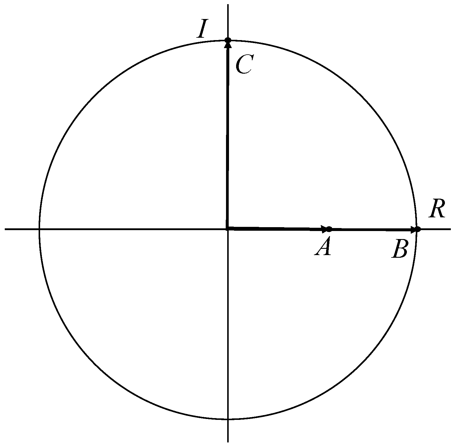
When we identify a particular signal out of several different signals, one of the most important step is measuring the difference between two complex fuzzy sets. Methods in [1,23] are combing the differences in the amplitude terms and the phase terms. For example, let $A=0.5/x$, $B=1/x$, and $C=e^{j0.5\pi }/x$, as shown in Figure 2 . Then we have $d(A,B)=d(B,C)$ by the method in [23]. However, in our point of view, the signal A is easier to be detected than the signal C for a given signal B, since A and B are in the same direction and B and C are orthogonal. To avoid this, our method to calculate the distance of two complex fuzzy sets is combing the differences in the in-phase terms and quadrature terms.

Let $S_l\left(t\right)$ ($1\le l\le L$) be L different signals. R is a given signal. Every $S_l\left(t\right)$ and $R\left(t\right)$ are sampled N times i.e., $1\le t\le N$.

Each signal $S_l\left(t\right)$ can be represented as:

$$S_l\left(t\right)=\frac{1}{N}\sum _{n=1}^N{C}_{l,n}·e^{j\frac{2\pi (n-1)(t-1)}{N}+a_{l,n}}$$

where $C_{l,n}$ are the complex Fourier coefficients $S_l$.

Then $S_l\left(t\right)$ can be rewritten in the form:

$$S_l\left(t\right)=\frac{1}{N}\sum _{n=1}^N{A}_{l,n}·e^{j\frac{2\pi (n-1)(t-1)}{N}+a_{l,n}}$$

where $C_{l,n}=A_{l,n}·e^{j{a}_{l,n}}$, with $A_{l,n}$, $a_{l,n}$ real-valued and $A_{l,n}\ge 0$ for all n ($1\le n\le N$).

Similarly, let $C_{R,n}$ be the Fourier coefficients of R, the signal $R\left(t\right)$ can be represented as:

$$R\left(t\right)=\frac{1}{N}\sum _{n=1}^N{A}_{R,n}·e^{j\frac{2\pi (n-1)(t-1)}{N}+a_{R,n}}$$

where $C_{R,n}=A_{R,n}·e^{j{a}_{R,n}}$, with $A_{R,n}$, $a_{R,n}$ real-valued and $A_{R,n}\ge 0$ for all n ($1\le n\le N$).

Apply the following method to compare the different signals.

Step 1

Normalize the amplitudes of all Fourier coefficients. Let ${\mathbf{A}}_l=(A_{l,1},A_{l,2},...,A_{l,N})$ be the vector of amplitudes of $S_l$’s Fourier coefficients, ($1\le l\le L$). Let ${\mathbf{A}}_R=(A_{R,1},A_{R,2},...,A_{R,N})$ be the vector of amplitudes of $S_R$’s Fourier coefficients, ($1\le l\le L$). Let ${\mathbf{B}}_l$ be the normalized vector $1/norm\left({\mathbf{A}}_l\right)·{\mathbf{A}}_l$, where $norm\left({\mathbf{A}}_l\right)=\sqrt{{\Sigma }_{n=1}^N{\left(A_{l,n}\right)}^2}$. Let ${\mathbf{B}}_R$ be the normalized vector $1/norm\left({\mathbf{A}}_R\right)·{\mathbf{A}}_R$. Then ${\mathbf{B}}_l=(B_{l,1},B_{l,2},...,B_{l,N})$ is the vector of normalized amplitudes of $S_l$’s Fourier coefficients. ${\mathbf{B}}_R=(A_{R,1},A_{R,2},...,A_{R,N})$ is the vector of normalized amplitudes of R’s Fourier coefficients.

Step 2

Composition the t samples $S_l\left(t\right)$, $1\le t\le N$ for each signal $S_l$ ($1\le l\le L$). Define new complex fuzzy sets as:

$$\begin{array}{c}\hfill B_l{e}^{a_l}=B_{l,1}\oplus B_{l,2}\oplus \cdots \oplus B_{l,n}{e}^{a_{l,1}\otimes a_{l,2}\otimes \cdots \otimes a_{l,N}}\end{array}$$

(31)

Similarly, define a new complex set as:

$$\begin{array}{c}\hfill B_R{e}^{a_R}=B_{R,1}\oplus B_{R,2}\oplus \cdots \oplus B_{R,n}{e}^{a_{R,1}\otimes a_{R,2}\otimes \cdots \otimes a_{R,N}}\end{array}$$

(32)

Step 3

For each $B_l$ ($1\le l\le L$), define its in-phase and quadrature terms, respectively, as:

$$\begin{array}{c}\hfill I_l=B_l\cos \left(a_l\right)\end{array}$$

(33)

and

$$\begin{array}{c}\hfill Q_l=B_l\sin \left(a_l\right).\end{array}$$

(34)

Similarly, define R’s in-phase and quadrature terms, respectively, as:

$$\begin{array}{c}\hfill I_R=B_R\cos \left(a_R\right)\end{array}$$

(35)

and

$$\begin{array}{c}\hfill Q_R=B_R\sin \left(a_R\right).\end{array}$$

(36)

Step 4

Calculate the distance between $S_l$ ($1\le l\le L$) and R:

$$\begin{array}{c}\hfill d(S_l,R)=\frac{1}{2}\max \left(\right|I_R-I_l|,|Q_R-Q_l\left|\right)\end{array}$$

(37)

Step 5

In order to conclude if $S_l$ may be identified as R, compare $1-d(S_l,R)$ to a threshold $\delta$. If $1-d(S_l,R)$ exceeds the threshold, identify $S_l$ as R.

Above Step 1 is the same as that in [1]. Other steps are different. Some complex fuzzy operations are used in Step 2. The Sum, Max, Min, and Winner Take All methods may be better than others for ⊗ in Step 2 , since these operations have the orthogonality preserving property (see Theorems 4, 5, 7 and 8). Step 3 is the orthogonal decomposition method, which is known as orthogonal demodulation in digital signal processing.

Example 7.

Two discrete time signals are represented by:

$$\begin{array}{c}\hfill S_1\left(t\right)=\frac{1}{5}\sum _{n=1}^5{A}_{R,n}·e^{j\frac{2\pi (n-1)(t-1)}{5}+\frac{\pi }{6}},t=1,2,...,5,\\ \hfill S_2\left(t\right)=\frac{1}{5}\sum _{n=1}^5{A}_{R,n}·e^{j\frac{2\pi (n-1)(t-1)}{5}+\frac{2\pi }{3}},t=1,2,...,5.\end{array}$$

respectively. The given signal R is:

$$\begin{array}{c}\hfill R\left(t\right)=\frac{1}{5}\sum _{n=1}^5{A}_{R,n}·e^{j\frac{2\pi (n-1)(t-1)}{5}},t=1,2,...,5.\end{array}$$

Assume that ⊕ is $Max$ and ⊗ is $Sum$. By applying Eqs.(31)-(32), we have $1/5e^{\frac{5\pi }{6}}$, $1/5e^{\frac{4\pi }{3}}$ and $1/5$. According to Equations (33)–(36), we obtain:

$$\begin{array}{c}\hfill d(S_1,R)=0.05,d(S_2,R)=0.15\end{array}$$

If $\delta =0.9$, identify $S_1$ as R.

In order to illustrate the superiority of the proposed method, a comparison between the proposed method and the existing methods [1,23] is conducted based on the numerical cases. By the method in Reference [1], we have same distance between $S_l(l=1,2)$ and R in the above Example 7. It is impossible to know which signal is more likely to be identified, which cannot satisfy the application of signal detection. Method in Reference [23] has same problem (see the example of Figure 2). Therefore, we can say that our proposal is a satisfactory method.

4. Discussion and Conclusions

In this paper, we introduced the orthogonality of complex fuzzy sets. We presented several results on orthogonality with respect to complex fuzzy operations and complex fuzzy inference method. The Sum, Max, Min, and Winner Take All methods in determining the phase term of the complex fuzzy union (intersection) have the orthogonality preserving property (see Theorems 4, 5, 7 and 8). A signal detection method was presented. In some special cases where some of the existing methods cannot provide reasonable results, the proposed method shows great capacity for discriminating complex fuzzy sets. Moreover, this method uses the choice of operations that have the orthogonality preserving property. However, our proposed method is not an absolutely perfect one. It is stuck with a lack of theoretical support. Furthermore, we have not show that Equation (37) in our method is a distance measure. Further efforts include continuing to look for a more excellent method (or distance measure) for much better exploration and exploitation on complex fuzzy sets.

Complex fuzzy sets, described in [1], are viewed as vectors in the complex plane, rather than scalar quantities. We should measure the difference of complex fuzzy sets from the viewpoint of vector theory. This idea of membership vectors induces new properties of complex fuzzy sets which are quite different from the properties of fuzzy set. Dick [16] analyzed the idea of rotational invariance for complex fuzzy logic. They also use figure of vector in complex plane to illustrate this point visibility. It is interesting to study complex fuzzy sets and complex fuzzy logic from the viewpoint of vector theory.

As we know, various orthogonal data are often applied in image processing and signal processing. The concept of orthogonality of complex fuzzy sets may be useful in these applications. Therefore, it will be meaningful to further discuss.

References

- Ramot, D.; Milo, R.; Friedman, M.; Kandel, A. Complex fuzzy sets. IEEE Trans. Fuzzy Syst. 2002, 10, 171–186. [Google Scholar] [CrossRef]
- Chen, Z.; Aghakhani, S.; Man, J.; Dick, S. ANCFIS: A Neuro-Fuzzy Architecture Employing Complex Fuzzy Sets. IEEE Trans. Fuzzy Syst. 2011, 19, 305–322. [Google Scholar] [CrossRef]
- Li, C. Complex Neuro-Fuzzy ARIMA Forecasting. A New Approach Using Complex Fuzzy Sets. IEEE Trans. Fuzzy Syst. 2013, 21, 567–584. [Google Scholar] [CrossRef]
- Li, C.; Chiang, T.-W. Complex Fuzzy Computing to Time Series Prediction A Multi-Swarm PSO Learning Approach. Lect. Notes Comput. Sci. 2011, 6592, 242–251. [Google Scholar]
- Li, C.; Chiang, T.-W. Intelligent financial time series forecasting: A complex neuro-fuzzy approach with multi-swarm intelligence. Int. J. Appl. Math. Comput. Sci. 2012, 22, 787–800. [Google Scholar] [CrossRef]
- Li, C.; Chiang, T.-W.; Yeh, L.-C. A novel self-organizing complex neuro-fuzzy approach to the problem of time series forecasting. Neurocomputing 2013, 99, 467–476. [Google Scholar] [CrossRef]
- Ma, J.; Zhang, G.; Lu, J. A method for multiple periodic factor prediction problems using complex fuzzy sets. IEEE Trans. Fuzzy Syst. 2012, 20, 32–45. [Google Scholar]
- Yazdanbakhsh, O.; Krahn, A.; Dick, S. Predicting solar power output using complex fuzzy logic. In Proceedings of the Joint IFSA World Congress and NAFIPS Annual Meeting, Edmonton, AB, Canada, 24–28 June 2013. [Google Scholar]
- Li, C.; Chiang, T.-W. Function Approximation with Complex NeuroFuzzy System Using Complex Fuzzy Sets. A New Approach. New Gener. Comput. 2011, 29, 261–276. [Google Scholar] [CrossRef]
- Li, C.; Chiang, T.-W. Complex fuzzy model with PSO-RLSE hybrid learning approach to function approximation. Int. J. Int. Inf. Database Syst. 2011, 5, 409–430. [Google Scholar] [CrossRef]
- Li, C.; Chiang, T.-W. Complex Neuro-Fuzzy Self-learning Approach to Function Approximation. Lect. Notes Comput. Sci. 2010, 5991, 289–299. [Google Scholar]
- Li, C.; Chan, F. Complex-Fuzzy Adaptive Image Restoration. An Artificial-Bee-Colony-Based Learning Approach. Lect. Notes Comput. Sci. 2011, 6592, 90–99. [Google Scholar]
- Li, C.; Wu, T.; Chan, F.-T. Self-learning complex neuro-fuzzy system with complex fuzzy sets and its application to adaptive image noise canceling. Neurocomputing 2012, 94, 121–139. [Google Scholar] [CrossRef]
- Dick, S.; Yager, R.; Yazdanbahksh, O. On Pythagorean and Complex Fuzzy Set Operations. IEEE Trans. Fuzzy Syst. 2016, 24, 1009–1021. [Google Scholar] [CrossRef]
- Tamir, D.E.; Jin, L.; Kandel, A. A new interpretation of complex membership grade. Int. J. Intell. Syst. 2011, 26, 285–312. [Google Scholar] [CrossRef]
- Dick, S. Towards Complex Fuzzy Logic. IEEE Trans. Fuzzy Syst. 2005, 13, 405–414. [Google Scholar] [CrossRef]
- Ramot, D.; Friedman, M.; Langholz, G.; Kandel, A. Complex fuzzy logic. IEEE Trans. Fuzzy Syst. 2003, 11, 450–461. [Google Scholar] [CrossRef]
- Tamir, D.E.; Kandel, A. Axiomatic theory of complex fuzzy logic and complex fuzzy classes. Int. J. Comput. Commun. Control 2011, 4, 562–576. [Google Scholar] [CrossRef]
- Tamir, D.E.; Last, M.; Kandel, A. Generalized complex fuzzy propositional logic. In Proceedings of the World Conference on Soft Computing, San Francisco, CA, USA, 23–26 May 2011. [Google Scholar]
- Tamir, D.E.; Last, M.; Kandel, A. The Theory and Applications of Generalized Complex Fuzzy Propositional Logic. In Soft Computing: State of the Art Theory and Novel Applications; Springer: Berlin, Germany, 2013; pp. 177–192. [Google Scholar]
- Tamir, D.E.; Teodorescu, H.N.; Last, M.; Kandel, A. Discrete complex fuzzy logic. In Proceedings of the Annual Meeting of the North American Fuzzy Information Processing Society (NAFIPS), Berkeley, CA, USA, 6–8 August 2012; pp. 1–6. [Google Scholar]
- Alkouri, A.U.M.; Salleh, A.R. Linguistic variables, hedges and several distances on complex fuzzy sets. J. Intell. Fuzzy Syst. 2014, 26, 2527–2535. [Google Scholar]
- Zhang, G.T.; Dillon, S.; Cai, K.-Y.; Ma, J.; Lu, J. Operation properties and δ-equalities of complex fuzzy sets. Int. J. Approx. Reason. 2009, 50, 1227–1249. [Google Scholar] [CrossRef]
- Zhang, G.; Dillon, T.S.; Cai, K.-Y.; Ma, J.; Lu, J. Delta-Equalities of Complex Fuzzy Relations. In Proceedings of the IEEE International 24th Conference on Advanced Information Networking and Applications, Perth, Australia, 20–23 April 2010; pp. 1218–1224. [Google Scholar]
- Scott, M. L. Programming Language Pragmatics, 2nd ed.; Morgan Kaufmann: Burlington, MA, USA, 2005. [Google Scholar]
- Alci, M. Fuzzy rule-base driven orthogonal approximation. Neural Comput. Appl. 2008, 17, 501–507. [Google Scholar] [CrossRef]
- Wang, L.; Langari, R. Building Sugeno-type models using fuzzy discretization and orthogonal parameter estimation technique. IEEE Trans. Fuzzy Syst. 1995, 3, 454–458. [Google Scholar] [CrossRef]
- Yen, J.; Wang, L. Simplification of fuzzy rule based systems using orthogonal transformation. In Proceedings of the Sixth IEEE International Conference of Fuzzy Systems, Barcelona, Spain, 5 July 1997; pp. 253–258. [Google Scholar]
- Mastorocostas, P.A.; Theocharis, J.B. An orthogonal least-squares method for recurrent fuzzy-neural modeling. Fuzzy Sets Syst., 2003, 140, 285–300. [Google Scholar] [CrossRef]
- Wang, L.X.; Mendel, J.M. Fuzzy basis functions, universal approximation, and orthogonal least squares learning. IEEE Trans. Neural Netw. 1992, 3, 807–814. [Google Scholar] [CrossRef] [PubMed]
- Kim, C.H.; Lee, C.W. Fuzzy control algorithm for multi-objective problems by using orthogonal array and its application to an AMB system. In Proceedings of the IFSA World Congress and, Nafips International Conference, Vancouver, BC, Canada, 25–28 July 2001; Volume 3, pp. 1752–1757. [Google Scholar]
- Kim, C.H.; Lee, C.W. Self-Organizing Fuzzy Controller for Multi-Objective Problem by Using Orthogonal Array and its Applications. Jpn. Soc. Mech. Eng. 2002, 277–282. [Google Scholar] [CrossRef]
Figure 1.
Orthogonality.
Figure 2.
Membership vectors A, B, and C.
© 2017 by the authors. Licensee MDPI, Basel, Switzerland. This article is an open access article distributed under the terms and conditions of the Creative Commons Attribution (CC BY) license (http://creativecommons.org/licenses/by/4.0/).
Share and Cite
MDPI and ACS Style
Hu, B.; Bi, L.; Dai, S. The Orthogonality between Complex Fuzzy Sets and Its Application to Signal Detection. Symmetry 2017, 9, 175. https://doi.org/10.3390/sym9090175
AMA Style
Hu B, Bi L, Dai S. The Orthogonality between Complex Fuzzy Sets and Its Application to Signal Detection. Symmetry. 2017; 9(9):175. https://doi.org/10.3390/sym9090175
Chicago/Turabian StyleHu, Bo, Lvqing Bi, and Songsong Dai. 2017. "The Orthogonality between Complex Fuzzy Sets and Its Application to Signal Detection" Symmetry 9, no. 9: 175. https://doi.org/10.3390/sym9090175
Note that from the first issue of 2016, this journal uses article numbers instead of page numbers. See further details here.