A Sparse Signal Reconstruction Method Based on Improved Double Chains Quantum Genetic Algorithm


College of Information and Communication Engineering, Harbin Engineering University, Harbin 150001, China
*
Author to whom correspondence should be addressed.
Symmetry 2017, 9(9), 178; https://doi.org/10.3390/sym9090178
Submission received: 11 August 2017
/
Revised: 30 August 2017
/
Accepted: 31 August 2017
/
Published: 2 September 2017
Abstract
:This paper proposes a novel method of sparse signal reconstruction, which combines the improved double chains quantum genetic algorithm (DCQGA) and the orthogonal matching pursuit algorithm (OMP). Firstly, aiming at the problems of the slow convergence speed and poor robustness of traditional DCQGA, we propose an improved double chains quantum genetic algorithm (IDCQGA). The main innovations contain three aspects: (1) a high density quantum encoding method is presented to reduce the searching space and increase the searching density of the algorithm; (2) the adaptive step size factor is introduced in the chromosome updating, which changes the step size with the gradient of the objective function at the search points; (3) the quantum -gate is proposed in chromosome mutation to overcome the deficiency of the traditional NOT-gate mutation with poor performance to increase the diversity of the population. Secondly, for the problem of the OMP algorithm not being able to reconstruct precisely the effective sparse signal in noisy environments, a fidelity orthogonal matching pursuit (FOMP) algorithm is proposed. Finally, the IDCQGA-based OMP and FOMP algorithms are applied to the sparse signal decomposition, and the simulation results show that the proposed algorithms can improve the convergence speed and reconstruction precision compared with other methods in the experiments.
1. Introduction
Signal decomposition and expression comprise a fundamental problem in the theory research and engineering application of signal processing. The traditional signal decomposition methods are decomposing the signals into a set of complete orthogonal bases, such as cosine transform bases, Fourier transform bases, wavelet transform bases, and so on. However, these decomposition methods suffer from inherent limitations for different kinds of signals [1]. For example, due to the lack of resolution ability in the time domain of the Fourier transform, the local component of the non-stationary signal has difficulty finding a correspondence of the Fourier coefficient. Therefore, Mallat et al. proposed a new signal decomposition method based on over-complete bases, which is called sparse decomposition or sparse reconstruction [2]. Compared with complete orthogonal bases, the over-complete bases (or redundant dictionary) are redundant, that is the number of base elements is larger than that of the dimensions. In this case, the orthogonality between the bases will no longer be guaranteed, and the bases are renamed atoms. The purpose of sparse reconstruction is to select as few atoms as possible in a given redundant dictionary to represent the signal succinctly. The selection process of atoms is also called the optimal atomic selection. Because the sparse decomposition can adaptively reconstruct the sparse signals using atoms in the dictionary, it has been widely applied in many aspects, such as signal denoising [3], feature recognition [4], weak signal extraction [5] and data compression [6]. At present, the most commonly-used sparse decomposition methods are the greedy algorithms based on global searching, for instance matching pursuit (MP), OMP, stage-wise orthogonal matching pursuit (StOMP), adaptive matching pursuit (SAMP), regularized orthogonal matching pursuit (ROMP), compressed sampling matching pursuit (CoSaMP), and so on [7,8,9,10,11]. The OMP algorithm and its variants are the theoretic basis of greedy algorithms, and they have become the focus of researchers. However, although sparse decomposition involving the greedy algorithm can reconstruct the original signals with the redundant dictionary, the computational complexity is too heavy to be implemented. Especially in a noisy environment with unknown signal sparsity, each searching step of the optimal atom requires many complex inner products’ calculations, which has become the biggest obstacle to the industrial application of sparse decomposition. There are mainly two kinds of methods that can solve the above problem: one is modifying the OMP algorithm and the redundant dictionary according to the specific characteristics of the signals [12], and the other is combining with artificial intelligence methods to search the optimal atoms [13,14,15,16,17,18,19]. Due to the rapid convergence and general applicability of a variety of signals, most existing sparse decomposition algorithms adopt the latter method.
The artificial intelligence search algorithm is an efficient global optimization method, which has strong universality and adaptability for parallel processing [14,15,16,17]. Each search process of the optimal atom is actually a global optimization problem, so the intelligent search algorithm can be applied to sparse decomposition to improve the search efficiency of the optimal atom. At present, the commonly-used intelligent search algorithms in sparse decomposition are the genetic algorithm (GA) [18,19,20], particle swarm optimization (PSO) [21,22,23] the and quantum optimization algorithm [24,25,26,27,28,29,30]. Among numerous optimization algorithms, the quantum genetic algorithm (QGA) is a new intelligent search algorithm, which combines GA and quantum information theory to complete global optimization [24,25,26,27]. As a branch of the QGA, the DCQGA has been one of the burning research problems in recent years, due to its small population size, strong searching ability and fast convergence speed [28,29,30]. However, the DCQGA has its own shortcomings: first of all, DCQGA with a large encoding space range affects the convergence rate; secondly, the initial iteration step size is needed for the quantum updating strategy, and the selection of the initial step size affects the convergence accuracy; finally, the chromosome mutation is treated by the NOT-gate, but it usually cannot achieve the purpose of increasing the population diversity.
In this paper, aiming at the deficiencies of the DCQGA, we propose an IDCQGA, which modifies the double chains encoding, the chromosome updating and the mutation of DCQGA, respectively. Then, a FOMP algorithm for the noisy signal without known sparsity is proposed. Finally, the IDCQGA is introduced into the optimal atomic selection of the FOMP algorithm to complete the sparse signal decomposition.
2. Data Models of the Redundant Dictionary and FOMP Algorithm
2.1. Redundant Dictionary
A key concern for sparse signal reconstruction is how to design efficient redundant dictionaries. There are many redundant dictionaries such as Gabor, wavelet packets, cascade of wavelets and sinusoidal functions, local cosine, and so on [2,3]. In this paper, we use Gabor atoms to generate the Gabor redundant dictionary for sparse reconstruction. Gabor atoms are chosen because they can provide the global and local characteristics of the time and frequency domains of the sparse signal at the same time [2]. Therefore, it is often applied as the basic structure of the redundant dictionary in the time-frequency atom processing methods. A Gabor atom in the redundant dictionary consists of a modulated Gauss window function:
where represents the Gauss window function. s, u, v and w represent scale, translation, frequency and phase of the atom, respectively. The Gabor redundant dictionary can be formed by stretching (s), translating (u) and modulating (v,w) a Gabor atom. is a set of the time frequency parameters, which can be discretized in the following ways [2]: where ; ; ; ; ; ; ; . The Gabor dictionary has a high redundancy, assuming the signal length is Nand the atomic number is . The purpose of this paper is to design the algorithms for atom selection and signal reconstruction, by selecting as few atoms as possible in the Gabor redundant dictionary to approximate the sparse signal.
2.2. OMP
Matching pursuit (MP) is a typical greedy algorithm that decomposes the signal into a linear expression of the optimal atoms that are selected from a redundant dictionary; while another greedy algorithm, the OMP, inherits the atomic selection rules of the MP algorithm. The difference is that selected atoms are processed by the Gram–Schmidt orthogonal method, and then, the residual signals are projected on the orthogonal atoms, which can improve the convergence of the algorithm [8]. The main procedures of the OMP algorithm are:
Step 1: In the redundant dictionary, we choose the optimal atom that matches the original signal f by:
where represents the inner product operation and is the redundant dictionary.
Step 2: Let ; normalize; then, f can be decomposed into:
where is the projection of f in and represents residual signal after the first decomposition of f.
Step 3: Continue to decompose the residual signal; select the optimal atom in the k-th decomposition:
Step 4: The Gram–Schmidt orthogonal algorithm is applied to :
Step 5: Normalize ; we get ; then, the residual signal can be decomposed into:
As the number of iterations k increases, after the K-th decomposition, the energy of the residual signal converges to zero [8]. The approximate representation of f can be obtained:
From the above steps, we know that the traditional OMP algorithm uses the hard threshold method by setting a large iteration K to get the signal sparse approximation or selects less than a given threshold as the iteration termination condition. However, in complicated noisy environments, the threshold is hard to define to make the energy of the residual signal contain only the noise signal instead of converging to zero. Therefore, an adaptive OMP algorithm is enlightened and proposed in the next section.
2.3. The Proposed FOMP Algorithm
Generally, the noisy sparse signal is composed of the effective signal components and the noise components. The effective signal components are the sparse components in the noisy sparse signal, and the Gabor atoms can be used to reconstruct them [2]. If the signal energy is applied to measure the number of decomposed atoms (iteration times K), for the sparse signal without noise, the greater the number of decomposed atoms, the smaller the energy of the residual signal. However, for the noisy sparse signal, with the continuous extraction of effective signals, too many atoms will reconstruct the noise components. By contrast, if the number of atoms is too small, it will lose some useful information; thus, the reconstructed signal cannot accurately approximate the effective components. To solve this problem, this paper proposes an FOMP algorithm that fully considers the fidelity of the reconstructed signal.
The Gabor atoms dictionary does not contain the atoms that match the Gauss white noise, so when the noisy sparse signal is decomposed, the atom that has the highest correlation with the effective signal is extracted firstly. With the increasing of the number of iterations, the correlation between the residual signal and the dictionary gets weaker and weaker. Assume f and are the noisy sparse signal and residual signal after the k-th iteration, respectively. f can be decomposed into:
where is the effective signal components. is the frequency band of the . and are the noise in the frequency range and the noise outside of the frequency range.
When the OMP method is used to decompose the signal, , and all atoms in the dictionary are orthogonal because is the noise outside of [8], the energy of residual signal after the k-th iteration is:
Similarly, the energy of residual signal after the -th iteration is:
According to the exact refactoring theory of the MP algorithm [2,8], converges exponentially to zero, i.e.,
where K is the iteration times, u is a coherent coefficient of the Gabor atoms dictionary and:
The traditional OMP algorithms select less than a given threshold as iteration termination condition. However, when the signal-to-noise ratio (SNR) is low, the value of the is relatively large, which reduces the the effectiveness of the traditional algorithms. In this paper, we find that the difference between the residual signal of the k-th and -th iterations can eliminate the noise term , and the difference will exponentially converge to zero,
According to Equation (13), we know that the difference between the residual signals can be used as a crucial factor of the iteration termination condition when using the OMP method to decompose the signal. Therefore, we define the fidelity:
where the numerator is the energy of the matched signal in the -th iteration, and the denominator is the energy of residual signal after the -th iteration. If the matched signal is precisely the remaining effective components in the -th iteration, then the residual signal contains only noise components, and is the critical point to separate the effective signal and noise. Therefore, the fidelity represents the energy ratio of the effective and noise components, and is the energy ratio of the noise and residual noise components. When the effective signal energy is much larger than the noise, will be far less than , and in the subsequent iterations, remains stable. Based on the analysis above, set the fidelity threshold ; when , the effective signal is accurately approximated, and the number of decomposed atoms is the sparsity of the original signal.
3. IDCQGA-Based FOMP Algorithm
DCQGA contains three key technologies: quantum bit (qubit) encoding, chromosome updating and mutation. In this paper, aiming at the defects of the three technologies, we propose an IDCQGA with a high density of search space, an adaptive update step size and the quantum -gate, which modifies the encoding method, the chromosome updating and mutation of DCQGA, respectively. The IDCQGA has higher search efficiency and robustness than the traditional DCQGA.
3.1. The Principle of DCQGA
3.1.1. Double Chains Qubit Encoding
DCQGA applies double chains quantum bits for encoding chromosomes. In the quantum computation, the smallest unit of information is the qubit [29]. The state of a qubit can be described as:
where and represent two basis states of the qubit and is the quantum superposition state. and are, respectively, the probability amplitudes of the two basis states and , . In DCQGA, a pair of probability amplitudes is represented by , where , and is a random number between zero and one. Therefore, double chains encoding for the i-th chromosome can be expressed as:
where and are the cosine chain encoding and sine chain encoding, respectively. , , . m represents the population size (the number of chromosomes); n is the number of qubits. The probability amplitudes of the qubit in each chromosome are periodically varied, which repeat in the unit circle in the process of updating, and the value range is with the encoding space being . However, such a large search space will affect the convergence rate of the algorithm.
3.1.2. Quantum Rotation Gate Updating
In DCQGA, the quantum rotation gate is used to update the qubit phase. Quantum rotation gate is defined as:
where is the rotation angle, and the updating process can be expressed as:
where: and: are the probability amplitudes before and after updating the j-th qubit in the i-th chromosome, respectively. The direction and step size of are crucial, which can directly affect the speed and search efficiency of the algorithm. For the direction of , it can be obtained by the following formula:
where and are the probability amplitudes of a qubit in the global optimal solution and and are the probability amplitudes of the corresponding qubits in the current solution. When , the direction of is ; when , the direction of the can be positive or negative.
For the step size of , according to [25,29], we know that the when , the change rate of is very small, which reduces the convergence speed and efficiency of the algorithm. When , it is easy to cause premature convergence. The literature [25,29] gives that the range of is , but does not provide a basis for the selection. Meanwhile, the current literature obtains the step size without considering the differences of the chromosomes and the change trend of the objective function.
3.1.3. Quantum Chromosome Mutation
In order to reduce the probability of prematurity and increase the diversity of the population, the mutation process is introduced by the quantum -gate in the traditional DCQGA. The -gate is defined as:
The mutation effect of the -gate for the j-th qubit in the i-th chromosome is:
Since and , therefore, the -gate mutation method is actually a swap of two bits of the genes in the chromosome and does not effectively increase the diversity of the population.
3.2. The Proposed IDCQGA
3.2.1. High Density Qubit Encoding
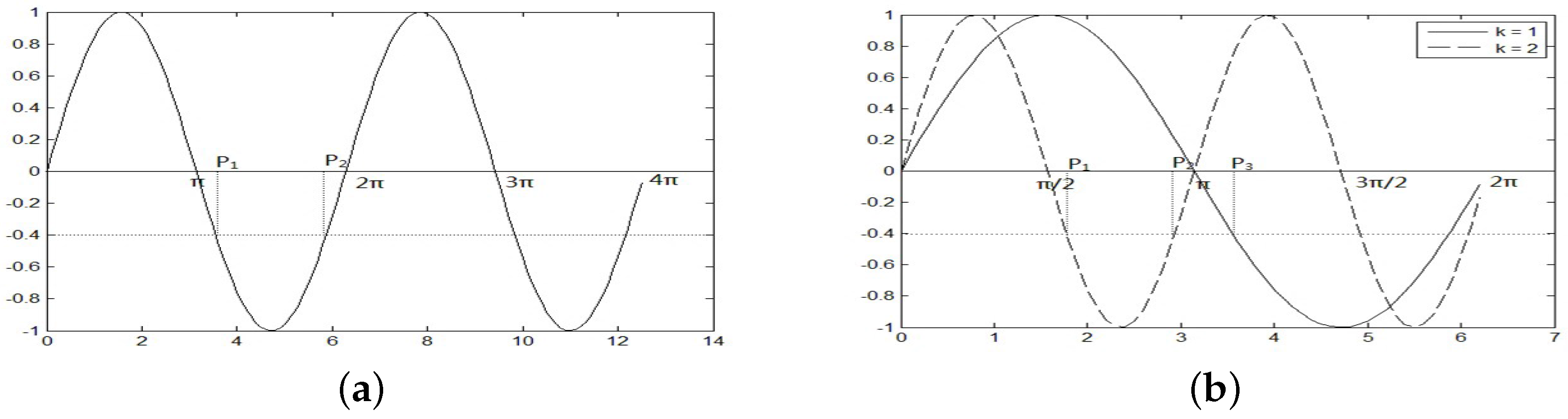
For simplicity, consider the sine chain temporarily. We reduce the range of encoding space firstly by limiting the phase angle of the probability amplitude to , so , and the range of the probability amplitude is still in . The improved encoding method ensures the monotonicity between the phase angle and the probability amplitudes. Meanwhile, it compresses the encoding space, namely it improves the density of the probability amplitude. However, a smaller encoding space will reduce the search probability of the optimal solution, as shown in Figure 1a. From Figure 1a, we know that when the encoding space is , and the corresponding probability amplitude is ; there are two phase solutions and . If the encoding space is , the corresponding phase solution is only , which will reduce the probability of searching the global optimal solution. Therefore, we introduce an adjustment factor kduring encoding to compensate for this deficiency, the improved double chains encoding method is shown as:
where the adjustment factor kis an integer greater than or equal to one. When , Equation (22) is the traditional double chains encoding; when , the adjustment factor compresses the period of the probability amplitude function and improves the probability of searching the global optimal solution. As shown in Figure 1b, when and the encoding space is in the range of , the phase angle corresponding to the probability amplitude of is only ; when , the encoding space is also , the phase angles corresponding to the probability amplitude of are and . This improved encoding method improves the search density and the probability of searching the global optimal solution under the premise of ensuring the search range.
In theory, the probability of searching the global optimal solution increases with the increasing of k. However, when k is too large, it will affect the convergence speed. After weighing the advantages and disadvantages, the adjustment factor k is chosen as three in this paper. The improvement of the encoding method is called high density qubit encoding, which increases the density of the search space and improves the searching probability.
3.2.2. Adaptive Step Size for Updating
In IDCQGA, we propose an adaptive step size quantum gate update method. The rotation angle is adjusted according to the changing of the fitness function at the search point (a single gene chain). When the change rate of the fitness function is large at the search point, the search step size is reduced appropriately. Conversely, it is appropriate to increase the search step size. Considering that the objection function is differentiable, the relative change rate (gradient) of the objective function is introduced into the rotation step size function. Define:
where is the gradient of the objective function at the point , and and are defined as:
where represents the j-th components of the vector in the solution space, m is the population size and n represents the number of bits in a single chromosome.
Based on the above-mentioned strategy of rotation angle and the step size range given by [24,28], in IDCQGA, the rotation angle function is defined as:
The defined rotation angle function possesses two advantages. One is that the defined brings the adaptive step size changes in the effective range of , which can ensure the validity of the chromosome updating. Another is that the step size is adaptively adjusted when the gradient of the objective function changes. In other words, such a modified method can make each chromosome jog in escarpment during the search procedure to avoid missing the global optimum solution and stride in plainness during the search procedure to accelerate convergence.
3.2.3. Quantum -Gate for Mutation
In IDCQGA, the -gate mutation is proposed and defined as follows:
The mutation effect of the -gate for the j-th qubit in the i-th chromosome is:
From the above formulas, we can see that the -gate mutation strategy is also a phase angle rotation, but this rotation changes the amplitude of the qubit, thus increasing the diversity of the population. Besides, although the -gate mutation has achieved promising results in this paper, it is important to note that we are not claiming that is the best angle to mutate the chromosome. Readers can make appropriate adjustments of the angle according to different experiments.
3.3. FOMP Algorithm Combined with IDCQGA
This section gives the implementation steps of the FOMP algorithm based on IDCQGA for sparse decomposition: is the group of parameters to be optimized in atom ; the inner product of the residuals signals and the atoms as the fitness function of the optimization algorithm; the fidelity threshold as the iterative termination condition of the FOMP algorithm.
Step 1: Set the parameters for the FOMP algorithm. Construct the Gabor atoms dictionary according to Equation (1), and initialize the residual signal and fidelity threshold .
Step 2: Initialize the quantum population. According to Equation (22), use the proposed high density encoding method to generate m chromosomes. Set the evolutionary generations and mutation probability .
Step 2.1: Transform the solution space. Each chromosome contains two chains, and each chain contains four probability amplitudes (four parameters in ). Using linear transform, probability amplitudes from the four-dimensional unit space can be mapped to the solution space ( and are the bounds of the parameters) of the optimize problem. After transformation, each chain corresponding to a solution, each probability amplitude corresponding to an optimal variable of the solution.
Step 2.2: Compute the fitness function. Get the inner products of the residuals signal and the atoms, namely obtain the fitness value of each chromosome according to Equation (4). Record the current optimal solution and the corresponding optimal chromosome .
Step 2.3: Update and mutate the chromosome. Update the population by the quantum rotation gate, and mutate the population by the quantum -gate. Determine the rotation angle according to Equation (26). Make the as the object, and update each qubit in the chromosome by using the quantum rotation gate. According to Equation (28) and the mutation probability , the mutation operation is performed on the new chromosome to obtain a new generation of chromosomes.
Step 2.4: Return to Step 2.1 and loop the processes for the new generation of the chromosome until it satisfies the evolutionary generations of IDCQGA.
Step 3: Calculate the fidelity . According to Equation (14), when fidelity , Equations (5) and (6) are applied to update the signal residuals, and then, return to Step 2. Otherwise, the FOMP iterative termination condition is satisfied; output the optimal solution, and restructure the signals.
4. Simulation Results and Analysis
The following experiments are performed in MATLAB 2012(a) using a Pentium(R) Processor G3260 + 3.3-GHz processor with the Windows 7 operating system. In order to prove the validity of the proposed algorithm in the noisy case, the average recovered signal-to-noise ratio (ASNR) and the root mean square error (RMSE) are defined, which are presented as:
where and represent the i-th source and restored signal. A larger ASNR or RMSE indicates higher accuracy of the restored signals.
4.1. Experiment 1 and Analysis: Performance of the IDCQGA
To show the performance of the IDCQGA, an optimization experiment of Shaffer’s F6function is designed, and the IDCQGA is compared with PSO [28], GA [20], QGA [26] and conventional DCQGA [29]. Shaffer’s F6 can be expressed as:
The three-dimensional surface of Shaffer’s F6 function is as shown in Figure 2a. Figure 2b,c is the profiles of and . From Figure 2, we know that there is only one global maximum point and infinitely many local maximum points in the range of both variables, which are both in . The global maximum point and global maximum are and one, respectively. When the function value obtained by the optimization algorithms is more than , we consider that the global maximum is obtained. The parameter setting of IDCQGA and other algorithms is shown in Table 1. In order to make comparisons easier, the initial experimental settings are the same as [26]. For DCQGA and IDCQGA, parameter “bits of gene” is equal to the number of variables (x and y), so it is two. In IDCQGA, the initial rotation angle is not needed because our algorithm is adaptive according to Section 3.2.2. For the PSO algorithm, there are two additional scaling factors and , which represent the weights of the statistical acceleration that push each particle to the optimum position [28].
The optimization results of the five algorithms for Shaffer’s F6 function are shown in Table 2 and Figure 3. The simulation results show that the proposed IDCQGA in this paper has the highest efficiency and the best optimization results in the five algorithms. From Table 2, we know that only IDCQGA and DCQGA perform well, which have reached the convergence criteria. Meanwhile, IDCQGA is superior to the other three algorithms in both convergence speed and convergence accuracy, for which the best values of convergence and generation times are and 22, respectively. The PSO, GA and QGA fall into the local extreme point and lead to premature convergence of the algorithm.
From Figure 3, we can see that the PSO, GA and QGA algorithms fall into the local extrema, which corroborates the above conclusions. QGA is the first to fall into the local extremum. This is predictable because the QGA algorithm has a poor update and mutation effect, which leads to the premature convergence in complex function optimization. The PSO algorithm shows better performance than GA and QGA because of the memory function, but the convergence rate is slow. IDCQGA has a faster convergence rate than DCQGA, which means that the proposed encoding method improves the searching speed. At the same time, IDCQGA obtains the global optimal solution without getting into the local extremum, so demonstrating that the proposed update method and mutation are more reasonable and effective.
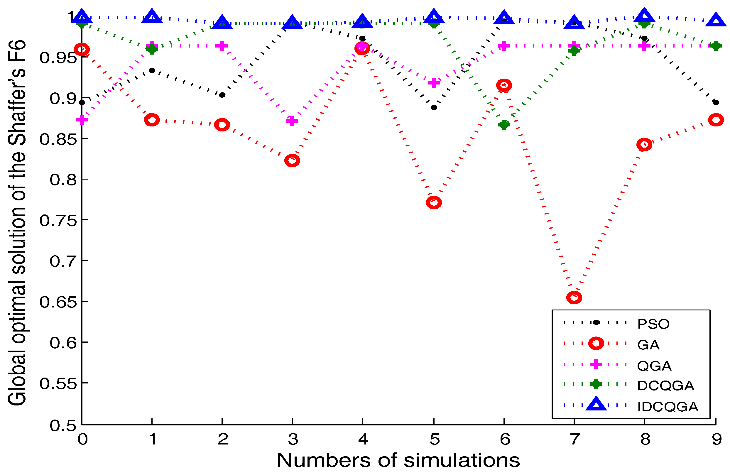
In order to verify the stability of the proposed IDCQGA, Shaffer’s F6 functions are optimized ten times by five algorithms, and the results are compared with the results of Table 3 and Figure 4. From the simulation results, we know that the optimization efficiency of the proposed IDCQGA algorithm is still the highest and basically consistent. Although the PSO and DCQGA algorithms can also achieve the purpose of optimization, the stability is poor. The above analysis shows that the proposed high density encoding, adaptive step size factor and the mutation gate can obviously improve the stability of the optimization algorithm.
4.2. Experiment 2 and Analysis: Performance of the OMP Based on IDCQGA
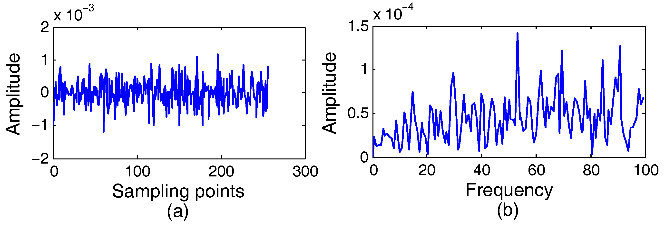
In this experiment, the effectiveness of the IDCQGA-based OMP algorithm is verified by using the real speech signal without noise. The sampling point is 20,000; the population size is 50; the evolution generation of IDCQGA is 100. In order to reduce the memory requirement of the algorithm, the speech signal is divided into frames, and each frame contains 256 sampling points. Take a frame of the speech signal. The original frame signal and the reconstruction frame signal using 100 atoms are shown in Figure 5. Figure 6 indicates the residual frame signal and frequency after the reconstruction. The original speech signal and the reconstructed speech signal are shown in Figure 7. The ASNR and RMSE of the reconstructed signal and the original signal are 38.6 dB and 0.025, respectively. It can be seen from the figures and results that the waveform and frequency of the reconstructed signal are similar to the source signal. The reason is that, in the noise-free signal environment, the more the iterations (more atoms reconstruct the signal) of the OMP algorithm based on IDCQGA, the smaller the residual signal and the more accurate the reconstructed signal.
The complexity analysis: For each frame of the speech signal, the traditional MP algorithm requires 119,756 (N is the number of sampling points) inner products’ operations to search each optimal Gabor atom, while the OMP algorithm needs more (k is the number of atoms in the current decomposition) inner products’ operations because of the orthogonal projection. Therefore, the fast convergence of OMP is based on the increase of the complexity. Because the IDCQGA does not involve the complex inner product operation in the optimization, the IDCQGA-based OMP algorithm requires (50 represents the population size, and 100 is the evolution generation) inner products’ operations to search each optimal Gabor atom, while the traditional OMP algorithm needs 119,756 inner products’ operations. Therefore, the proposed algorithm can obviously reduce the complexity of sparse decomposition with little sacrifice of the optimization quality.
4.3. Experiment 3 and Analysis: Performance of the FOMP Based on IDCQGA
In order to verify the stability of the IDCQGA-based FOMP algorithm in noisy environments, at first, we reconstruct one frame of the speech signal when the signal-to-noise ratio (SNR) is 20 dB and 30 dB. The relationship between the fidelity and the iterations is shown in Figure 8a. It can be seen from the graph that the fidelity presents an obvious jump after 36 iterations and then remains almost stable. This indicates that is greater than . That is, 36 is the adaptive iterative termination critical point when the SNRs are 20 dB and 30 dB. Figure 8b shows the trend of the RMSE between the reconstructed signal and the original signal with the increases of the number of atoms in the 20-dB and 30-dB SNR. It can be seen that the RMSE of the reconstructed signal decreases to the minimum when the atom index = 36. This can be explained by the principles of atomic analysis and FOMP: In each step of matching pursuit, by calculating the inner products of the atoms and residual signals, we choose the matching atoms with the largest (or relatively large) inner product, which is most relevant to the effective component. Therefore, the initially searched atoms must be the main components of the effective signal. With the increase of the number of atoms, the atomic correlation becomes smaller. When the signal is extracted from a certain number of atoms, the residual signal is almost all of the noise, the minimum RMSE is obtained. Additionally, RMSE increases again when the atom increases because too many atoms will reconstruct the noise components. At the same time, in this experiment, we can set the same fidelity threshold in different SNR situations, and this proves the high adaptiveness of the FOMP algorithm.
Under different SNR conditions, the average recovered signal-to-noise ratio (ASNR) is used as the evaluation index. Four algorithms are compared respectively to discuss the ASNR of the reconstructed signal. The results averaged over 50 Monte Carlo trials are shown in Figure 9. From the figures, we know that, in noisy environments, the four algorithms can achieve a similar and higher ASNR. At the same time, the IDCQGA is superior to the other three algorithms in the reconstruction accuracy. While performing this experiment, the CPU time is recorded to measure the computational complexity of each algorithm. The CPU times occupied by GA-FOMP, QGA-FOMP, DCQGA-FOMP and IDCQGA-FOMP in the 20-dB SNR are as follows: 2.30 s, 1.86 s, 1.53 s, 1.36 s. There are two main reasons that explain the above conclusions. One is that the proposed FOMP algorithms can be used to terminate the iteration at the critical point of the signal and noise under the condition of different SNRs. Thus, the four algorithms can all achieve a higher ASNR. The other is that the proposed high density encoding and adaptive update step in IDCQGA reduces the inner product computation and improves the convergence speed of the algorithm under the prerequisite of guaranteeing the optimization precision.
4.4. Experiment 4 and Analysis: The Applicability of the Proposed Algorithms for Radar Signals
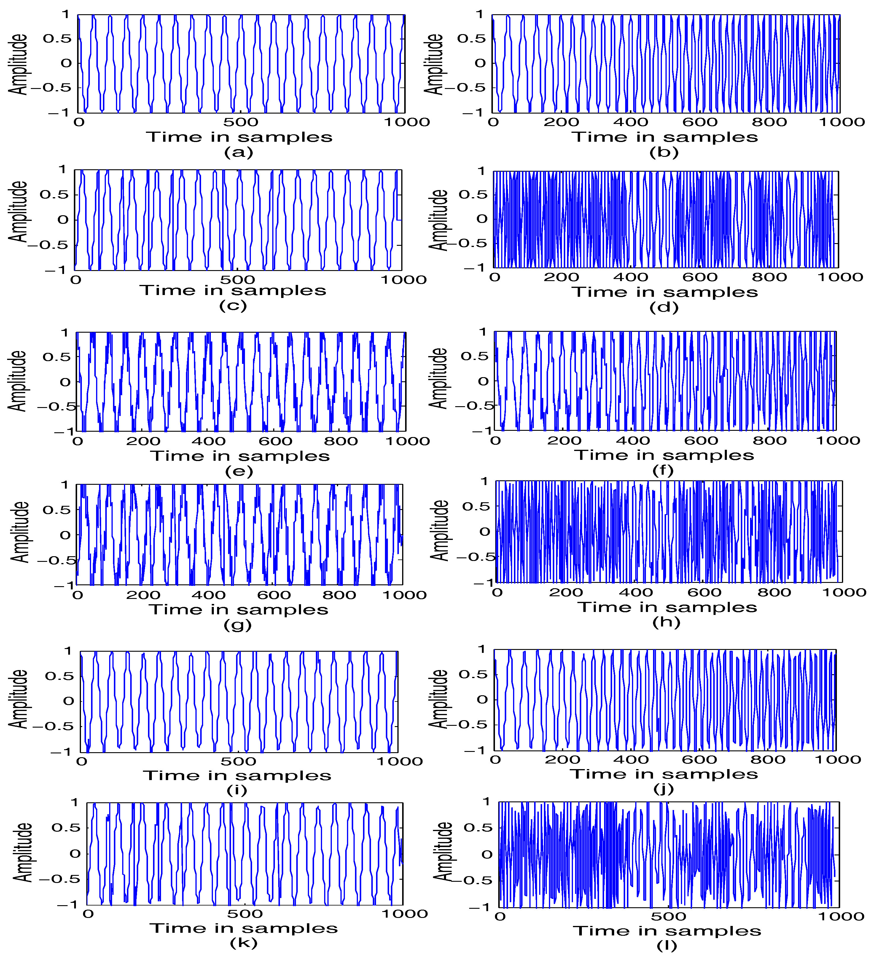
In this experiment, radar signals are utilized to verify the applicability and effectiveness of the Gabor decomposition method and the proposed algorithm. Four typical radar emitter signals,conventional pulse signal (CON), linear frequency modulated signal (LFM), binary phase coded signal (BPSK) and binary frequency coded signal (BFSK), are chosen for sparse reconstruction. The parameter settings are as follows: signal pulse width 10 s, LFM bandwidth 5 MHz; all of the rest of the signal carrier frequency is 2 MHz, except that the BFSK has two frequency points at 5 MHz and 10 MHz. BPSK and BFSK use a 13-bit Barker code. When the SNR is 15 dB, for each typical radar emitter signal, the IDCQGA-based FOMP algorithm is applied to reconstruct the signal with the fidelity threshold of . The original signal, the noisy signal and the reconstructed signal of the radar emitter signals are shown in Figure 10. It can be seen from Figure 10 that under the fidelity threshold conditions, by using the atomic decomposition of the typical radar emitter signals in the redundant dictionary, the extracted Gabor atoms can effectively restore the original signal, which can reflect the main features of the original signal. The applicability of the proposed algorithm to radar signals is verified.
In order to compare the effectiveness of the proposed method of the radar signal in different SNR environments, Table 4 lists the RMSE of the original signal with the noisy signal and the reconstructed signal. From Table 4, we know that the RMSE of the reconstructed signal and the original signal is significantly lower than the RMSE between the noisy signal and the original signal under different SNR conditions. It is proven that the characteristic parameters extracted from the noisy signal can be used to suppress the noise, and the proposed algorithms have better adaptability to the radar signals.
5. Conclusions
In this paper, an FOMP algorithm is proposed to solve the problem of the traditional OMP algorithm not being able to reconstruct effectively the signal in noisy environments. At the same time, due to the shortcomings of the DCQGA, we put forward an IDCQGA with the rapid and accurate optimization characteristics, which modifies the double chains encoding, the chromosome updating and mutation of DCQGA, respectively. Then, the IDCQGA and FOMP algorithm are combined to realize the sparse decomposition of a speech signal and radar signals. Compared with other methods in the experiments, the proposed algorithm can improve the convergence speed of the algorithm on the premise of ensuring the discriminability and fidelity of reconstructed signal. How to achieve better results under lower SNR conditions and how to solve the problem of weak sparse signal reconstruction in blind sources conditions is the next research direction.
Acknowledgments
This work is supported by the National Natural Science Foundation of China (No. 61371172), the International S&T Cooperation Program of China (ISTCP) (No. 2015DFR10220), the Ocean Engineering Project of the National Key Laboratory Foundation (No. 1213), the Fundamental Research Funds for the Central Universities (No. HEUCF1508) and the Natural Science Foundation of Heilongjiang Province (No. F201337).
Author Contributions
Qiang Guo and Guoqing Ruan conceived of and designed the study. Guoqing Ruan and Qiang Guo performed the experiments. Guoqing Ruan wrote the paper. Qiang Guo and Guoqing Ruan reviewed and edited the manuscript. All authors read and approved the manuscript.
Conflicts of Interest
The authors declare that there are no conflict of interests regarding the publication of this paper.
References
- Goodwin, M. Adaptive Signal Models: Theory, Algorithms, and Audio Applications. Ph.D. Thesis, University of California, Berkeley, CA, USA, 1997. [Google Scholar]
- Mallat, S.; Zhang, Z. Matching pursuit with time-frequeney dictionaries. IEEE Trans. Signal Process. 1993, 41, 3397–3415. [Google Scholar] [CrossRef]
- Xu, S.; Yang, X.; Jiang, S. A fast nonlocally centralized sparse representation algorithm for image denoising. Signal Process. 2016, 31, 99–112. [Google Scholar] [CrossRef]
- Xu, K.; Minonzio, J.G.; Ta, D.; Bo, H.; Wang, W.; Laugier, P. Sparse SVD method for high resolution extraction of the dispersion curves of ultrasonic guided waves. IEEE Trans. Ultrason. Ferroelectr. Freq. Control 2016, 63, 1514–1524. [Google Scholar] [CrossRef] [PubMed]
- Tang, H.; Chen, J.; Dong, G. Sparse representation based latent components analysis for machinery weak fault detection. Mech. Syst. Signal Process. 2014, 46, 373–388. [Google Scholar] [CrossRef]
- Wang, H.Q.; Ke, Y.L.; Song, L.Y.; Tang, G.; Chen, P. A sparsity-promoted decomposition for compressed fault diagnosis of roller bearings. Sensors 2016, 16, 1524. [Google Scholar] [CrossRef] [PubMed]
- Blumeusath, T.; Davies, M.E. Gradient pursuits. IEEE Trans. Signal Process. 2008, 56, 2370–2382. [Google Scholar] [CrossRef]
- Tropp, J.; Gilbert, A. Signal recovery from random measurements via orthogonal matching pursuit. IEEE Trans. Inf. Theory 2007, 53, 4655–4666. [Google Scholar] [CrossRef]
- Donoho, D.L.; Tsaig, Y.; Drori, I.; Starck, J.L. Sparse solution of underdetermined linear equations by stage-wise rthogonal matching pursuit. IEEE Trans. Inf. Theory 2012, 58, 1094–1121. [Google Scholar] [CrossRef]
- Needell, D.; Vershynin, R. Signal recovery from incomplete and inaccurate measurements via regularized orthogonal matching pursuit. IEEE J. Sel. Top. Signal Process. 2010, 4, 310–316. [Google Scholar] [CrossRef]
- Needell, D.; Tropp, J.A. CoSaMP: Iterative signal recovery from incomplete and inaccurate samples. Appl. Comput. Harmonic Anal. 2009, 26, 301–321. [Google Scholar] [CrossRef]
- Piro, P.; Sona, D.; Murino, V. Inner product tree for improved orthogonal matching pursuit. In Proceedings of the International Conference on Pattern Recognition, Tsukuba, Japan, 11–15 November 2012; pp. 429–432. [Google Scholar]
- Sun, T.Y.; Liu, C.C.; Tsai, S.J.; Hsieh, S.T.; Li, K.Y. Cluster guide particle swarm optimization (CGPSO) for underdetermined blind source separation with advanced conditions. IEEE Trans. Evolut. Comput. 2011, 15, 798–811. [Google Scholar] [CrossRef]
- Nasrollahi, A.; Kaveh, A. Engineering design optimization using a hybrid PSO and HS algorithm. Asian J. Civ. Eng. 2013, 14, 201–223. [Google Scholar]
- Nasrollahi, A.; Kaveh, A. A new hybrid meta-heuristic for structural design: Ranked particles optimization. Struct. Eng. Mech. 2014, 52, 405–426. [Google Scholar]
- Kaveh, A.; Nasrollahi, A. A new probabilistic particle swarm optimization algorithm for size optimization of spatial truss structures. Int. J. Civ. Eng. 2014, 12, 1–13. [Google Scholar]
- Saremi, S.; Mirjalili, S.; Lewis, A. Grasshopper optimisation algorithm: Theory and application. Adv. Eng. Softw. 2017, 105, 30–47. [Google Scholar] [CrossRef]
- Chen, X.; Liu, X.; Dong, S.; Liu, J. Single-channel bearing vibration signal blind source separation method based on morphological filter and optimal matching pursuit (MP) algorithm. J. Vib. Control 2015, 21, 1757–1768. [Google Scholar] [CrossRef]
- Wang, J.; Wang, L.; Wang, Y. Seismic signal fast decomposition by multichannel matching pursuit with genetic algorithm. In Proceedings of the IEEE International Conference on Signal Processing, Beijing, China, 21–25 October 2012; pp. 1393–1396. [Google Scholar]
- Ventura, R.F.I.; Vandergheynst, P. Matching Pursuit through Genetic Algorithms; LTS-EPFL tech. report 01.02; Signal Processing Laboratories: Lausanne, Switzerland, 2001. [Google Scholar]
- Guldogan, M.B.; Arikan, O. Detection of sparse targets with structurally perturbed echo dictionaries. Digit. Signal Process. 2013, 23, 1630–1644. [Google Scholar] [CrossRef] [Green Version]
- Li, C.; Su, Y.; Zhang, Y.; Yang, H. Root imaging from ground penetrating radar data by CPSO-OMP compressed sensing. J For. Res. 2017, 28, 1–8. [Google Scholar] [CrossRef]
- Xu, C.; Zhang, P.; Wang, H.; Li, Y.; Lv, C. Ultrasonic echo wave shape features extraction based on QPSO-matching pursuit for online wear debris discrimination. Mech. Syst. Signal Process. 2015, 60, 301–315. [Google Scholar] [CrossRef]
- Narayanan, A.; Moore, M. Quantum-inspired genetic algorithms. In Proceedings of the IEEE International Conference on Evolutionary Computation, Nagoya, Japan, 20–22 May 1996; pp. 61–66. [Google Scholar]
- Yang, J.A.; Li, B.; Zhuang, Z.Q. Multi-universe parallel quantum genetic algorithm its application to blind-source separation. In Proceedings of the IEEE international conference on neural networks and signal processing, Nanjing, China, 14–17 December 2003; pp. 393–398. [Google Scholar]
- Dahi, Z.A.E.M.; Mezioud, C.; Draa, A. A quantum-inspired genetic algorithm for solving the antenna positioning problem. Swarm Evolut. Comput. 2016, 31, 24–63. [Google Scholar] [CrossRef]
- Xiong, G.; Hu, Y.X.; Tian, L.; Lan, J.L.; Jun-Fei, L.I.; Zhou, Q. A virtual service placement approach based on improved quantum genetic algorithm. Front. Inf. Technol. Electron. Eng. 2016, 17, 661–671. [Google Scholar] [CrossRef]
- Chen, P.; Yuan, L.; He, Y.; Luo, S. An improved SVM classifier based on double chains quantum genetic algorithm and its application in analogue circuit diagnosis. Neurocomputing 2016, 211, 202–211. [Google Scholar] [CrossRef]
- Li, P.C.; Song, K.P.; Shang, F.H. Double chains quantum genetic algorithm with application to neuro-fuzzy controller design. Adv. Eng. Softw. 2011, 42, 875–886. [Google Scholar] [CrossRef]
- Kong, H.; Ni, L.; Shen, Y. Adaptive double chain quantum genetic algorithm for constrained optimization problems. Chin. J. Aeronaut. 2015, 28, 214–228. [Google Scholar] [CrossRef]
Figure 1.
Schematic diagrams of the coding space. (a) The traditional coding space; (b) the improved coding space when k = 1 and k = 2.
Figure 1.
Schematic diagrams of the coding space. (a) The traditional coding space; (b) the improved coding space when k = 1 and k = 2.

Figure 2.
Shaffer’s F6 function. (a) Three-dimensional surface; (b) profile of y=0; (c) profile of x=0.
Figure 2.
Shaffer’s F6 function. (a) Three-dimensional surface; (b) profile of y=0; (c) profile of x=0.
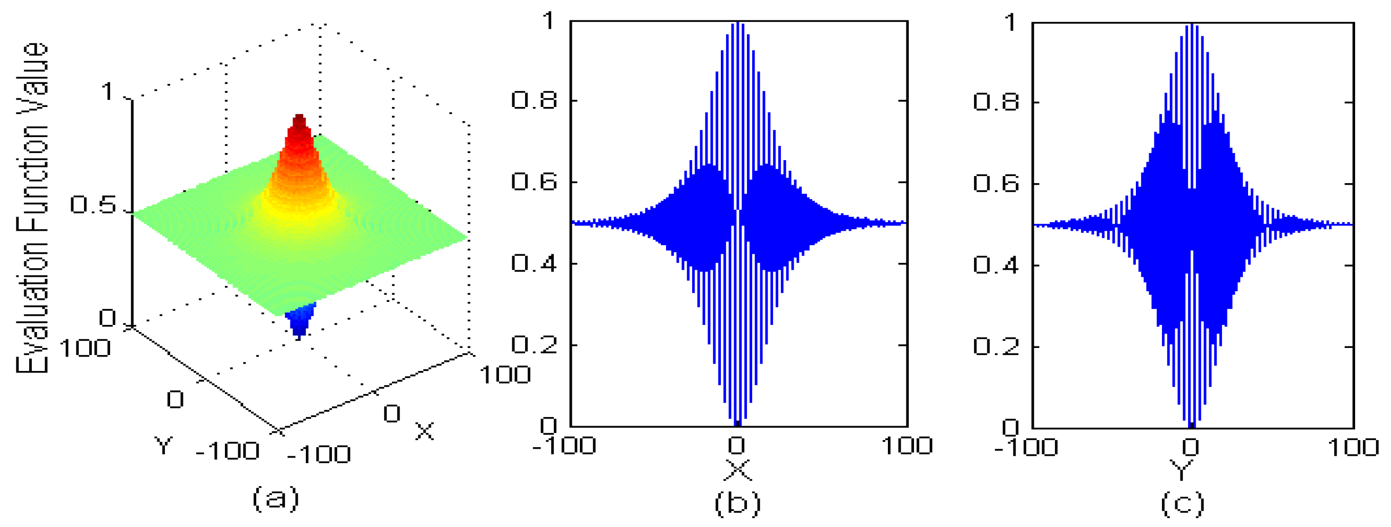
Figure 3.
Relationship between global optimization results and evolutionary generation.
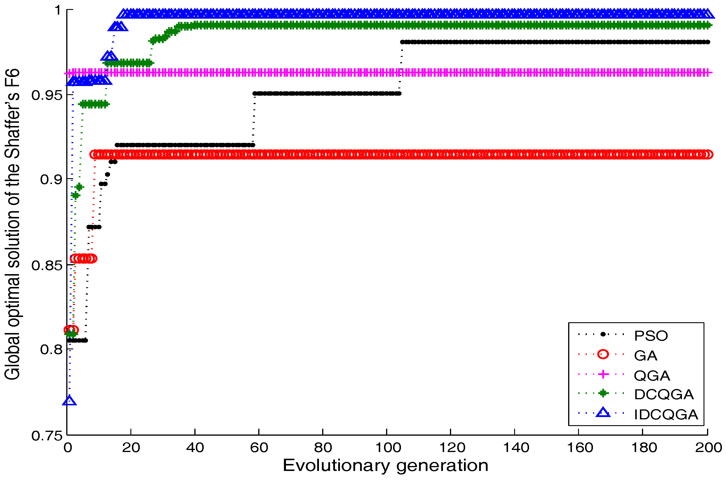
Figure 4.
The comparison of the optimization results of Shaffer’s F6.

Figure 5.
The original frame signal and the reconstruction frame signal using 100 atoms. (a) The original frame signal; (b) the original frequency frame signal; (c) the reconstruction frame signal; (d) the reconstruction frequency frame signal.
Figure 5.
The original frame signal and the reconstruction frame signal using 100 atoms. (a) The original frame signal; (b) the original frequency frame signal; (c) the reconstruction frame signal; (d) the reconstruction frequency frame signal.
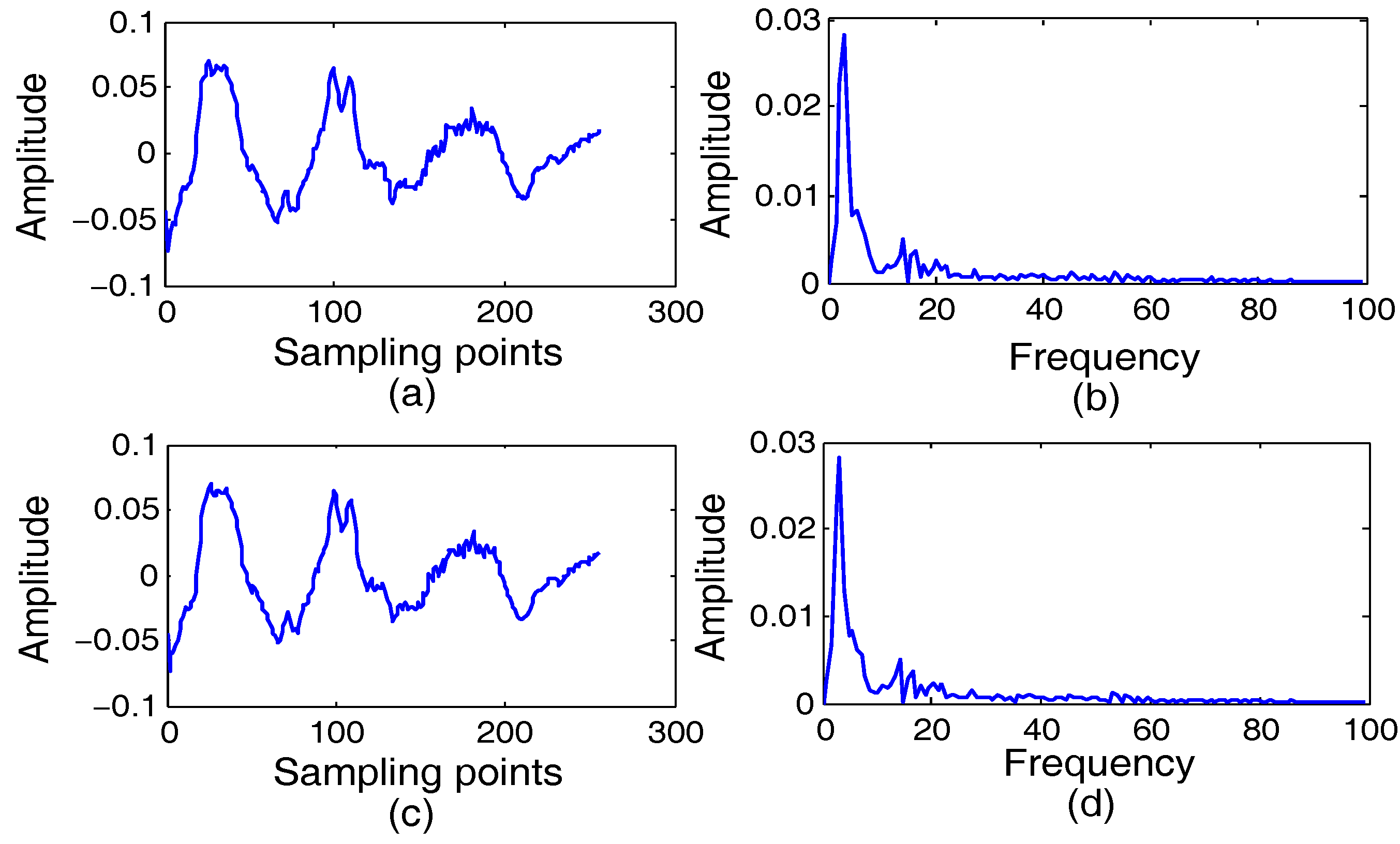
Figure 6.
The residual frame signal and residual frequency after the reconstruction. (a) The residual frame signal; (b) the residual frequency after the reconstruction
Figure 6.
The residual frame signal and residual frequency after the reconstruction. (a) The residual frame signal; (b) the residual frequency after the reconstruction

Figure 7.
The original speech signal and the reconstructed speech signal using the IDCQGA-based OMP algorithm. (a) The original speech signal; (b) the reconstructed speech signal.
Figure 7.
The original speech signal and the reconstructed speech signal using the IDCQGA-based OMP algorithm. (a) The original speech signal; (b) the reconstructed speech signal.
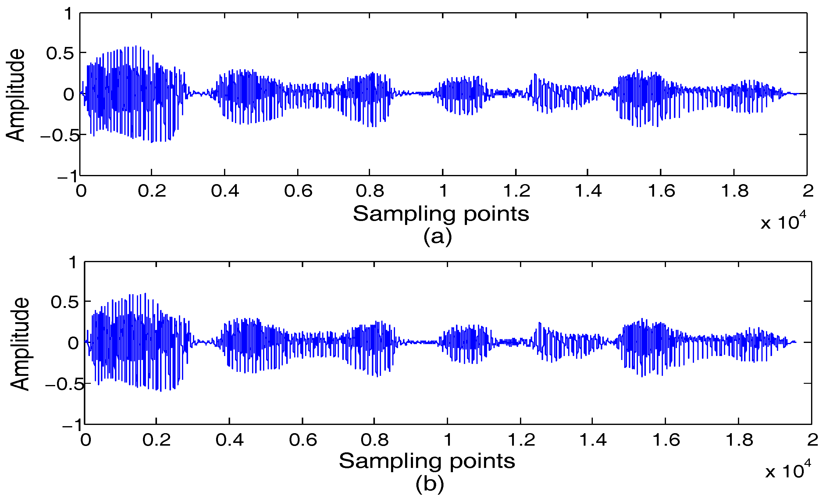
Figure 8.
Performance of the OMP based on IDCQGA. (a) The relationship between the fidelity and the iterations; (b) the relationship between the RMSE and the number of atoms.
Figure 8.
Performance of the OMP based on IDCQGA. (a) The relationship between the fidelity and the iterations; (b) the relationship between the RMSE and the number of atoms.

Figure 9.
The ASNR of the reconstructed signal with different SNRs. FOMP, FOMP.

Figure 10.
The original signal, the noisy signal and the reconstructed signal of the radar emitter signals. (a) The original signal of CON; (b) the original signal of LFM; (c) the original signal of BPSK; (d) the original signal of BFSK; (e) the noisy signal of CON; (f) the noisy signal of LFM; (g) the noisy signal of BPSK; (h) the noisy signal of BFSK; (i) the reconstructed signal of CON; (j) the reconstructed signal of LFM; (k) the reconstructed signal of BPSK; (l) the reconstructed signal of BFSK.

Table 1.
Parameters setting of the improved double chains quantum genetic algorithm (IDCQGA) and other algorithms.
Table 1.
Parameters setting of the improved double chains quantum genetic algorithm (IDCQGA) and other algorithms.
| Algorithm | Population | Bits of | Encoding | Crossover | Mutation | Initial Rotation | Evolutionary |
|---|---|---|---|---|---|---|---|
| Size | Gene | Method | Probability | Probability | Angle | Generation | |
| PSO | 50 | - | - | - | - | - | 200 |
| GA | 50 | 100 | Binary | 0.7 | 0.05 | - | 200 |
| QGA | 10 | 100 | qubit | - | - | - | 200 |
| DCQGA | 10 | 2 | Double chains | - | 0.05 | 200 | |
| IDCQGA | 10 | 2 | High density | - | 0.05 | - | 200 |
Table 2.
The global optimization results of the four algorithms for Shaffer’s F6 function.
| Algorithm | x | y | Best Result | Convergent Generations |
|---|---|---|---|---|
| PSO | 2.7583 | 5.01376 | 0.98327 | 105 |
| GA | 8.0283 | 4.81177 | 0.91128 | 9 |
| QGA | 2.8985 | 5.5678 | 0.96278 | 1 |
| DCQGA | −2.6202 | −1.7276 | 0.99028 | 40 |
| IDCQGA | 1.51263 | 1.39374 | 0.99793 | 22 |
Table 3.
Ten times optimization results of the four algorithms for Shaffer’s F6 function.
| Algorithm | Best Result | Worst Result | Average Result | Number of Convergence |
|---|---|---|---|---|
| PSO | 0.9901 | 0.8925 | 0.9512 | 3 |
| GA | 0.9604 | 0.6545 | 0.8535 | 0 |
| QGA | 0.9628 | 0.8711 | 0.9402 | 0 |
| DCQGA | 0.9903 | 0.8666 | 0.9687 | 6 |
| IDCQGA | 1 | 0.9902 | 0.9946 | 10 |
Table 4.
The RMSE of the original signal with the noisy signal and the reconstructed signal.
| SNR | CON | LFM | BPSK | BFSK | |
|---|---|---|---|---|---|
| 5dB | Noisy signal | 0.6545 | 0.6531 | 0.6572 | 0.6496 |
| Reconstructed signal | 0.0530 | 0.0335 | 0.0402 | 0.0545 | |
| 10dB | Noisy signal | 0.5263 | 0.0372 | 0.0369 | 0.5302 |
| Reconstructed signal | 0.0324 | 0.0372 | 0.0369 | 0.0357 | |
| 15dB | Noisy signal | 0.4179 | 0.3986 | 0.3659 | 0.3982 |
| Reconstructed signal | 0.0213 | 0.0257 | 0.0315 | 0.0268 | |
| 20dB | Noisy signal | 0.3345 | 0.2856 | 0.3549 | 0.3058 |
| Reconstructed signal | 0.0197 | 0.0190 | 0.0204 | 0.0173 |
© 2017 by the authors. Licensee MDPI, Basel, Switzerland. This article is an open access article distributed under the terms and conditions of the Creative Commons Attribution (CC BY) license (http://creativecommons.org/licenses/by/4.0/).
Share and Cite
MDPI and ACS Style
Guo, Q.; Ruan, G.; Wan, J. A Sparse Signal Reconstruction Method Based on Improved Double Chains Quantum Genetic Algorithm. Symmetry 2017, 9, 178. https://doi.org/10.3390/sym9090178
AMA Style
Guo Q, Ruan G, Wan J. A Sparse Signal Reconstruction Method Based on Improved Double Chains Quantum Genetic Algorithm. Symmetry. 2017; 9(9):178. https://doi.org/10.3390/sym9090178
Chicago/Turabian StyleGuo, Qiang, Guoqing Ruan, and Jian Wan. 2017. "A Sparse Signal Reconstruction Method Based on Improved Double Chains Quantum Genetic Algorithm" Symmetry 9, no. 9: 178. https://doi.org/10.3390/sym9090178
Note that from the first issue of 2016, this journal uses article numbers instead of page numbers. See further details here.