An Internet of Things Approach for Extracting Featured Data Using AIS Database: An Application Based on the Viewpoint of Connected Ships

Abstract

Automatic Identification System (AIS), as a major data source of navigational data, is widely used in the application of connected ships for the purpose of implementing maritime situation awareness and evaluating maritime transportation. Efficiently extracting featured data from AIS database is always a challenge and time-consuming work for maritime administrators and researchers. In this paper, a novel approach was proposed to extract massive featured data from the AIS database. An Evidential Reasoning rule based methodology was proposed to simulate the procedure of extracting routes from AIS database artificially. First, the frequency distributions of ship dynamic attributes, such as the mean and variance of Speed over Ground, Course over Ground, are obtained, respectively, according to the verified AIS data samples. Subsequently, the correlations between the attributes and belief degrees of the categories are established based on likelihood modeling. In this case, the attributes were characterized into several pieces of evidence, and the evidence can be combined with the Evidential Reasoning rule. In addition, the weight coefficients were trained in a nonlinear optimization model to extract the AIS data more accurately. A real life case study was conducted at an intersection waterway, Yangtze River, Wuhan, China. The results show that the proposed methodology is able to extract data very precisely.

1. Introduction

The Automatic Identification System (AIS) is a broadcast-style communication system developed for exchanging navigational data automatically and autonomously. It was originally designed for ship collision avoidance and maritime regulatory, and now it is gradually being used as an important connected-ship technique by ship owners to monitor the ship location and cargos. The AIS communication network can be separated into two parts, the ship borne AIS station and the shore station. The ship borne AIS stations broadcast ship related static and dynamic information on Very High Frequency (VHF) band at regular frequency according to the International Telecommunication Union (ITU) specification. The static information, which is manually entered or updated, mainly include identifier, call sign, ship name, dimensions, type, etc. The dynamic information, which is from the Global Navigation Satellite System (GNSS), includes timestamp, Speed over Ground (SOG), Course over Ground (COG), position (present by longitude and latitude), etc. The shore stations are mainly set up by shore authorities. While the ship borne AIS station is sending out messages, ships and shore stations around can receive these messages and displaying them on Electrical Navigation Chart (ENC). Therefore, the AIS enables the communication between ships and shore authorities, and help the maritime administrators, ship owner, and ship pilot to detect the position and state of vessels.

According to the mandatory requirement of the Convention on the Safety of Life at Sea (SOLAS) convention in 2002, all ships of 300 gross tonnage and upwards engaged on international voyages, cargo ships of 500 gross tonnage and upwards not engaged on international voyages, as well as passenger ships irrespective of size shall be fitted with an AIS. Hence, the AIS became one of the most widely used pieces of equipment onboard. Because the AIS provides abundant ship voyage related information, it is recognized as the primary data source in maritime situation awareness. The AIS data is widely used in risk analyses, accident prevention, motion pattern recognition, route prediction, and anomaly detection, etc. Qu et al. [1] introduced the AIS database into quantitatively evaluating the collision risks in the Singapore Strait. Balmat et al. [2] proposed a fuzzy approach to assess the maritime risk at sea based on the decision-making system with the real AIS data. Wang et al. [3] exploited the contextual AIS data in a coupled spatial–temporal perspective microscopic analytical scheme for a two-vessel collision accident investigation. Mou et al. [4] made a statistical analysis for collision involved ships by using AIS data in Rotterdam Port to investigate the accurate and actual behavior of collision-involved ships. Ristic et al. [5] extracted motion patterns by the statistical analysis of the real historic AIS data, in order to construct the corresponding motion anomaly detectors of ships in ports and waterways. Pallotta et al. [6] proposed an unsupervised and incremental learning approach to extract maritime movement patterns, for the purpose of converting raw data to information supporting decisions, such as traffic route extraction and anomaly detection. In these previous studies, the extraction of valid data from the AIS database is always the primary and fundamental step. However, the extraction of valid data is also the most time-consuming and laborious task before conducting studies.

Many researchers gave their solutions on this problem. Demšar et al. [7] introduced a 3D space-time density of trajectories to visualizing the temporal-spatial data, and presented an application to vessels’ trajectories acquired by AIS. Scheepens et al. [8] proposed a method that can explore the attributes along trajectories by calculating a density field for multiple subsets of the data. In order to discover similar groups of sub-trajectories in the spatial database, Debnath et al. [9] proposed a framework to cluster sub-trajectories by combining techniques from grid based approaches, spatial geometry, and string processing. Kim et al. [10] developed a maritime traffic gridded database by projecting traffic data on a geographic coordinate system. However, in general, the grid-based methods for extracting AIS data need a prior definition on optimal grid size, which is difficult to get. To solve this problem, Arguedas et al. [11] proposed an algorithm to automatically produce hierarchical graph-based representations of maritime shipping lanes extrapolated from historical AIS data, but the grid-based method became inefficient as the scale expands. The improvement of grid-based methods on data classification and extraction is the vector-based methods. In this aspect, Gerben et al. [12] applied a piecewise linear segmentation method to compress the trajectories obtained from AIS data. Zhang et al. [13] use the Douglas-Peucker (DP) algorithm to simplify AIS trajectories by extracting the characteristic points. Compared with the grid-based method, the computational burden of the vector-based method decreased a lot indeed. However, these methods didn’t fully utilize the contents of the AIS data, such as the SOG, COG, etc. Xiao et al. [14] proposed a statistical approach to extracting ship traffic behaviors with AIS data, including spatial distribution, speed distribution, course distribution, average speed, and traffic density, the research contributed a lot for data extraction from the AIS database. Liu et al. [15] provides a solution for extracting anomaly movement in the maritime traffic domain based on the clustering, in the study, the position, SOG, and COG were utilized in extracting AIS data in tandem, i.e., the role of position, SOG, and COG in AIS data point are unrelated.

In daily administration, maritime administrators are capable of extracting featured AIS data according to their experience on dynamic attributes of the vessels, such as SOG, COG, and position. However, it is impossible and inefficient to extract the massive AIS data timely by manual labor. Referring to the procedure of vessel classification of maritime administrators, it is feasible to simulate the experiences of administrators based on artificial intelligence that should be able to make conjunctive inference with the SOG, COG, and position. Focused on the extraction of vessel targets in radar images, Ma et al. [16] given the similar cognition of building an artificial intelligence base on Bayesian Network. Therefore, building an artificial intelligence for extracting featured AIS data is a typical probabilistic inference issue applied in vessels’ spatial-temporal data. Based on the above analysis, a probabilistic methodology was proposed to classify ships with AIS dynamic information. The position, SOG, and COG are treated as pieces of evidence to make the final decision in a cooperative way. However, in contrast to the SOG and COG, the position is hard to be converted into pieces of evidence. Nevertheless, as the ship sailing in the waterway, the SOG and COG of the vessels would be featured. In consideration of the two factors, the trajectory evidence was discarded and the AIS data with the SOG and COG evidence was extracted. In this case, the computational burden of the AIS data will be decrease greatly.

The scope of this study is to propose an artificial intelligence for extracting featured data from the AIS database. The paper is organized as follows: Section 2 gives the proposed approach for extracting featured AIS data with validate samples. Section 3 delivers an application of the proposed approach, which located in the Wuhan waterway, middle stream of the Yangtze River. Finally, Section 4 contains the conclusions of this proposal.

2. A Proposed Approach

As mentioned above, this paper is dedicated to introducing the artificial intelligence of maritime administrators into extracting featured AIS data. The maritime administrators make their inferences on featured data according to their experience, which comes from the daily observation of massive vessels. The artificial intelligence is typically a kind of probabilistic inference [16].

Bayesian Inference is one of the most classical methodologies in the probabilistic inference domain, and it is capable of handling the noise data of moving targets [16]. However, the limitation of Bayesian Inference is that it requires the frame of discernment being mutually exclusive and independent. Dempster-Shafer (DS) theory is considered as an improvement of Bayes Inference, it is able to make rigorous probabilistic inference, which constitutes a conjunctive probabilistic process [17,18]. The reliabilities of evidences in DS theory are considered to be fully reliable. Hence, DS theory cannot combine two pieces of evidence in complete conflict [19]. To address this problem, Dezert et al. [20,21] developed the Dezert-Smarandache Theory (DSmT) by introducing coefficient of reliabilities and weights, and makes the DSmT capable of combining pieces of evidence in complete confliction by redistributing the conflicts of evidences. However, DSmT neither keeps the consistencies with the Bayesian rule, nor is acknowledged as rigorous reasoning [22]. Originated from the Dempster’s and Bayesian rule, Yang et al. [22] developed the Evidential Reasoning (ER) rule in which the coefficients of weight and reliability are inherited from DSmT, and their discounting method are modified, hence there is no more deficiency in the inference process, meanwhile keeping the consistency with the Bayesian rule. 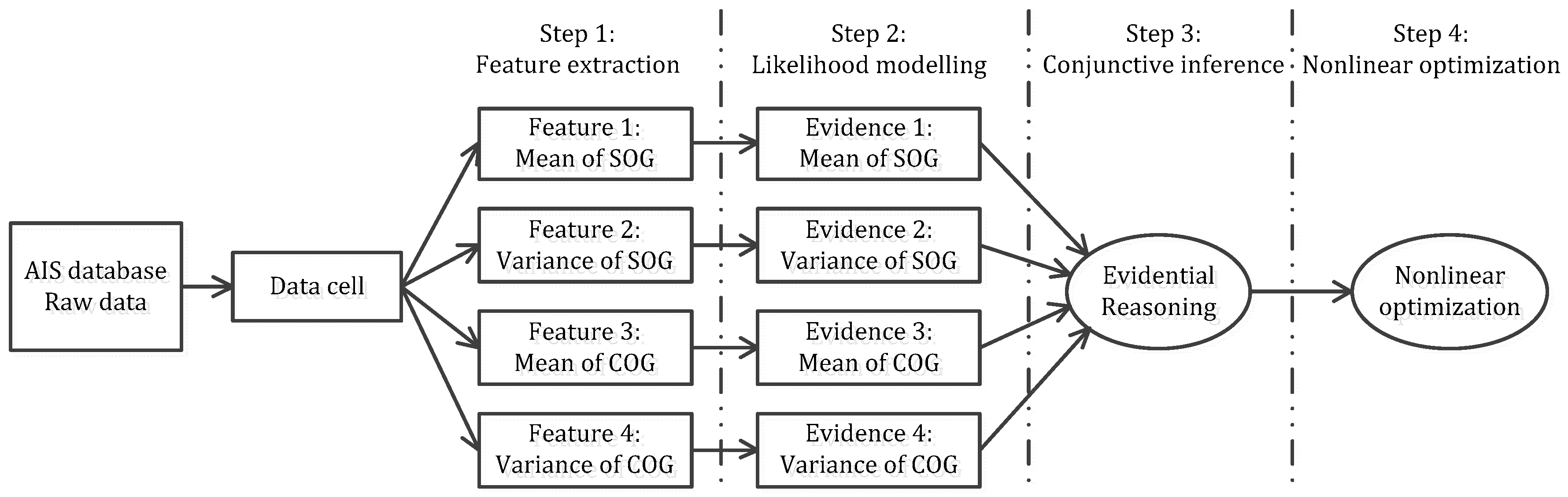Moreover, compared with the conventional Bayesian inference, the ER rule does not need the prior probability of patterns or states, because it constitutes a likelihood modelling [23]. Therefore, the ER rule provides a rigorous way to build the artificial intelligence of experienced maritime administrators. In this section, the details on introducing the ER rule into extracting featured AIS data will be present. The processing flow of the approach is depicted with four steps, including feature extracting, likelihood modeling, conjunctive inference, and nonlinear optimization on weights, as shown in Figure 1.

2.1. Step 1: Feature Extraction

In order to build an efficient probabilistic inference model, a quantity of AIS data samples should be gathered firstly. From the verified AIS data samples, dynamic attributes of vessels, such as SOG and COG, can be quantified and transformed to frequency distributions of mean and variance of SOG, and COG, respectively.

Suppose that there are m categories of data samples, and the data samples can be classified by making conjunctive inference of the mean and variance of SOG, COG. Then, the mean of SOG, variance of SOG, the mean of COG, and variance of COG are treated as four pieces of evidence for classifying data samples. Take the mean of SOG for example, in order to obtain the frequency distribution of mean of SOG of the data samples, the mean of SOG should be discretized. Suppose the minimum mean of SOG is v_min and the maximum mean of SOG is v_max, the range of mean of SOG is equally divided into L parts. Then, $y_i^j$ denotes the frequency or the number of times that the mean of SOG being equal to Value i for Class j, with i = 1, 2, …, L, j = 1, 2, …, m. Then, the total number of data samples for class j can be present as $Q^j={\displaystyle {\sum }_{i=1}^L{y}_i^j}$. As shown in

Table 1. Attribute values for verified sample in the hypotheses.

Classification	Verified Sample Attribute Distribution Value					Total
	Value 1	…	Value i	…	Value L
Class (1)	$y_1^1$	…	$y_i^1$	…	$y_L^1$	$Q^1={\displaystyle {\sum }_{i=1}^L{y}_i^1}$
Class (2)	$y_1^2$	…	$y_i^2$	…	$y_L^2$	$Q^2={\displaystyle {\sum }_{i=1}^L{y}_i^2}$
⋮	⋮	⋮	⋮	⋮	⋮	⋮
Class (j)	$y_1^j$	…	$y_i^j$	…	$y_L^j$	$Q^j={\displaystyle {\sum }_{i=1}^L{y}_i^j}$
⋮	⋮	⋮	⋮	⋮	⋮	⋮
Class (m)	$y_1^m$	…	$y_i^m$	…	$y_L^m$	$Q^m={\displaystyle {\sum }_{i=1}^L{y}_i^m}$

.

Similarly, the frequency distribution of variance of SOG, mean of COG, and variance of COG for the data samples can also be presented like Table 1.

2.2. Step 2: Likelihood Modelling

After acquiring the frequency distributions of ship motion attributes demonstrated present in Table 1, these characterized distributions should then be transferred to support degrees of the categories. That is to say, the mapping functions between support degrees and statistical distributions should be found out.

The concepts description of DS theory is introduced as follows. Suppose $\Theta =\left\{{\theta }_1,{\theta }_2,\cdots ,{\theta }_m\right\}$ is a set of mutually exclusive and collectively exhaustive propositions. Where ${\theta }_1,{\theta }_2,\cdots ,{\theta }_m$ denote to the categories, respectively. Let $\varphi$ represent the empty set. Then, $\Theta$ is referred to as a frame of discernment. The power set of $\Theta$ consists of $2^m$ subsets of $\Theta$, is denoted by $P(\Theta )$. Different from the conventional probabilistic inference methods, a belief degree or a probability might be also assigned to the power set $P(\Theta )$ in the ER rule when there is a reliability problem in evidence [22].

A Basic Probability Assignment (bpa) is a function p: $2^{\Theta }\to \left[0,1\right]$ that satisfies,

$$p\left(\varphi \right)=0,{\displaystyle {\sum }_{\theta \subseteq \Theta }p\left(\theta \right)}=1$$

(1)

where the basic probability $p\left(\theta \right)$ is assigned exactly to a proposition $\varphi$ and not to any smaller subset of $\varphi$. $p\left(\theta \right)$ is generated from the frequency distributions. Referring to the research conducted by Yang et al. [23], the likelihoods based on the frequency distributions can be presented as follows.

The core of likelihood modeling is to find the probabilistic relationships between the values of a frequency distribution and the classification (i.e., Class 1, Class 2, …, Class m) of a AIS data cell. The likelihood transformation approach established by Yang et al. [23] underpins a new likelihood modeling method for classifying vessels, which is described as follows.

Based on the frequency distributions given in Table 1, the likelihood that an attribute is equal to value i for a class j is calculated in Equation (2).

$$c_i^j=y_i^j/Q^{j}i=1,2,\cdots ,L,j=0,1,\cdots ,m$$

(2)

where $c_i^j$ denotes the likelihood to which attribute distribution is expected to be equal to value i in class j.

Let $p_i^j$ denote the probability that an attribute with value i points to class j, which is independent of the prior distribution of the classification. $p_i^j$ is then acquired as normalized likelihood as follows [23].

$$p_i^j=c_i^j/{\displaystyle {\sum }_{k=1}^m{c}_i^k}\hspace{1em}i=1,2,\cdots ,L,j=1,2,\cdots ,m$$

(3)

Belief distributions, given by Equation (3) represent the probabilistic relationships between the motion attributes and its classification. Note that a belief distribution reduces to a conventional probability distribution when $p_i^0$ is equal to zero, or there is no ambiguity about the classification. Following the above procedure, an attribute value can be mapped to a belief distribution, which is regarded as a piece of evidence.

2.3. Step 3: Conjunctive Inference

Subsequently, the ER rule is used to process these pieces of evidence, and it also takes the reliability and weight of evidence into considerations. A piece of evidence e_i is represented as a random set and profiled by a Belief Distribution (BD) as follows:

$$e_i=\left\{\left(\theta ,p_{\theta ,i}\right),\forall \theta \subseteq \Theta ,{\displaystyle {\sum }_{\theta \subseteq \Theta }{p}_{\theta ,i}}=1\right\}$$

(4)

where $\left(\theta ,p_{\theta ,i}\right)$ is an element of evidence e_i, representing that the evidence points to proposition $\theta$, which can be any subset of $\Theta$ or any element of $P(\Theta )$ except for the empty set, to the degree of $p_{\theta ,i}$, referred to as probability or degree of belief in general. $\left(\theta ,p_{\theta ,i}\right)$ is referred to as a focal element of e_i, if $p_{\theta ,i}>0$. In this occasion, $p_{\theta ,i}$ is exactly coming from the probabilities obtained from the quantified characterized distributions of different classification, given by Equations (2) and (3).

In addition, the reliability is associated with evidence e_i, denoted by r_i, which represents the ability of the evidence, where e_i is generated, to provide a correct assessment or solution for a given problem [21]. The reliability of a piece of evidence is the inherent property of the evidence, and in the ER framework it measures the degree of support for, or opposition to, a proposition given that the evidence points to the proposition. In other words, the unreliability of a piece of evidence sets a bound within which another piece of evidence can play a role in support for, and opposition against, different propositions. On the other hand, evidence e_i can also be associated with a weight, denoted by w_i. The weight of a piece of evidence shares the same definition as that of its reliability [22]. When different pieces of evidence are acquired from different sources, or measured in different ways, the weight of evidence can be used to reflect its relative importance in comparison with other evidence and determined according to who uses the evidence.

To combine a piece of evidence with another piece of evidence, it is necessary to take into account three elements of the evidence; its belief distribution (probability), reliability, and weight. In the ER rule, this is achieved by defining a so-called weight belief distribution with reliability as follows:

$$m_i=\left\{\left(\theta ,{\tilde{m}}_{\theta ,i}\right),\forall \theta \subseteq \Theta ;\left(P(\Theta ),{\tilde{m}}_{P(\Theta ),i}\right)\right\}$$

(5)

where ${\tilde{m}}_{\theta ,i}$ measures the degree of support for $\theta$ from e_i with both the weight and reliability of e_i taken into account, defined as follows:

$${\tilde{m}}_{\theta ,i}=\{\begin{array}{cc}0& \theta =\varphi \\ c_{rw,i}{m}_{\theta ,i}& \theta \subseteq \Theta ,\theta \ne \varphi \\ c_{rw,i}\left(1-r_i\right)& \theta =P(\Theta )\end{array}$$

(6)

$$c_{rw,i}=1/\left(1+w_i-r_i\right)$$

(7)

where $c_{rw,i}$ denotes a normalization factor, w_i denotes for weight, and r_i denotes reliability. $m_{\theta ,i}$ is the degree of support for proposition θ from evidence i, which is given by $m_{\theta ,i}=w_i{p}_{\theta ,i}$, with $p_{\theta ,i}$ being the degree of belief that evidence i points to θ. As described previously, $p_{\theta ,i}$ can be obtained using Table 1, Equations (2) and (3) $P(\Theta )$ is the power set of the frame of discernment Θ that contains all mutually exclusive hypotheses in question. It is worth mentioning that $P(\Theta )$ is treated as an independent element in the ER rule [22].

If every piece of evidence is fully reliable, e.g., r_i = 1 for any i, the ER rule reduces to Dempster’s rule. Evidences given by AIS are not fully reliable, so r_i < 1. The combination of two pieces of evidence e₁ and e₂ (defined in Equation (4)) will be conducted as follows:

$$p_{\theta ,e(2)}=\{\begin{array}{cc}0& \theta \subseteq \varphi \\ \frac{{\widehat{m}}_{\theta ,e(2)}}{{\displaystyle {\sum }_{D\subseteq \Theta }{\widehat{m}}_{D,e(2)}}}& \theta \subseteq \Theta \end{array}$$

(8)

$${\widehat{m}}_{\theta ,e\left(2\right)}=\left[\left(1-r_2\right)m_{\theta ,1}+\left(1-r_1\right)m_{\theta ,2}\right]+{\displaystyle {\sum }_{B\cap C=\theta }{m}_{B,1}{m}_{C,2}}\hspace{1em}\forall \theta \subseteq \Theta$$

(9)

where $m_{\theta ,1}$, $m_{\theta ,2}$, $m_{B,1}$ and $m_{\mathrm{C},2}$ are given by Equations (5)–(7); B, C and D denote any elements in the power set $P(\Theta )$ except for the empty set; the $p_{\theta ,e(2)}$ is the synthetic belief distribution to proposition $\theta$ when taking the two pieces of evidence e₁ and e₂ into consideration. Yang et al. [23] proved that the belief distribution here is equivalent to the probability in Bayesian rule if belief is assigned to singleton states only and $p_i^{\theta }$ is calculated by Equation (4). Therefore, the ER rule can be used to obtain the probability of an AIS data cell indicates to which classification, by using the mean and variance of SOG, COG extracted from the AIS data, respectively.

2.4. Step 4: Nonlinear Optimization

Weight coefficients were trained through a non-linear optimization, with verified samples to get a higher accuracy of classification. As discussed, in Equations (6) and (7), the reliability and weight of evidence are parameters used to measure evidence quality. In Step 2, the evidence from normalized likelihoods was generated independently of the prior distribution of hypotheses by assuming that each set of sample data is fully reliable.

In practice, the data provided by AIS is not completely reliable. Hence the evidences are not completely reliable either. As mentioned above, a weight of a piece of evidence is a relative importance which determined by whom is making the inference. In practice, such importance is exactly related to a verified sample and a certain optimization objective [23]. To a group of verified samples, appropriate weights of evidence should make the final result more likely to achieve a setting objective. Hence, appropriate weight coefficients can be obtained only if an objective and verified samples are determined.

A typical objective is set to minimize a global deviation. All of the classification results were compared with the reality, the aim of optimizing the weight coefficient is that, for a certain number of validated samples, the number of incorrect classification divide the number of validate samples, i.e., the error rate, is minimized. In fact, the global deviation in question generally includes the classification on object. Thus, a sign function is often used to determine a discrete state (usually true of false) of object based on their belief distributions (probability) to corresponding hypotheses. However, the sign function is very difficult to be modeled in related algorithms [24]. Hence, in this research, the weight coefficient can be solved in a compromised way as follows.

Let $S_j$ be the verified samples indicate to vessels belong to class j, where j = 1, 2, …, m. And N_j is the number of samples for class j. Let $S_j^k$ denotes the sample k in class j, where k = 1, 2, …, N_j. $p_{{\theta }_j,e}\left(S_j^k,w^T\right)$ denotes the probability to proposition ${\theta }_j$, where ${\theta }_j$ indicates to the class j. $p_{{\theta }_j,e}\left(S_j^k,w^T\right)$ is obtained by the conjunctive reasoning process using the ER rule. Thus, for each judgment on the sample $S_j^k$, the deviation can be presents as 1 − $p_{{\theta }_j,e}\left(S_j^k,w^T\right)$. All of the probability $p_{{\theta }_j,e}\left(S_j^k,w^T\right)$ share the same weight vector w^T = {w₁, w₂, w₃, w₄}, which denotes the weight coefficients of mean of SOG, variance of SOG, mean of COG, variance of COG, respectively. Hence, the global accuracy or sum of inferred probabilities that have been assigned to the correct propositions is presented as,

$$\varphi \left(w^T\right)={\displaystyle {\sum }_{j=1}^m{\displaystyle {\sum }_{k=1}^{N_j}\left[1-p_{{\theta }_j,e}\left(S_j^k,w^T\right)\right]}}$$

(10)

To minimize the deviation, w^T should make Equation (10) minimum. Therefore, the optimization formulation can be presented as,

$$w^T=\arg {\min }_{w^T:feasible}\varphi \left(w^T\right)$$

(11)

As discussed, without a sign function, this optimization can only provide a compromised solution to weights. Since Equation (10) is continuous and derivable, Equation (11) can be solved with the ‘fmincon’ function of MATLAB. With this procedure, more appropriate weights of pieces of evidence can be solved. Actually, the weights of pieces of evidence can also be set through optimizing other objectives, depending on the requirements, for example, to achieve a higher accuracy of class 1. Other optimization objectives will be discussed in the following case study.

3. A Case Study

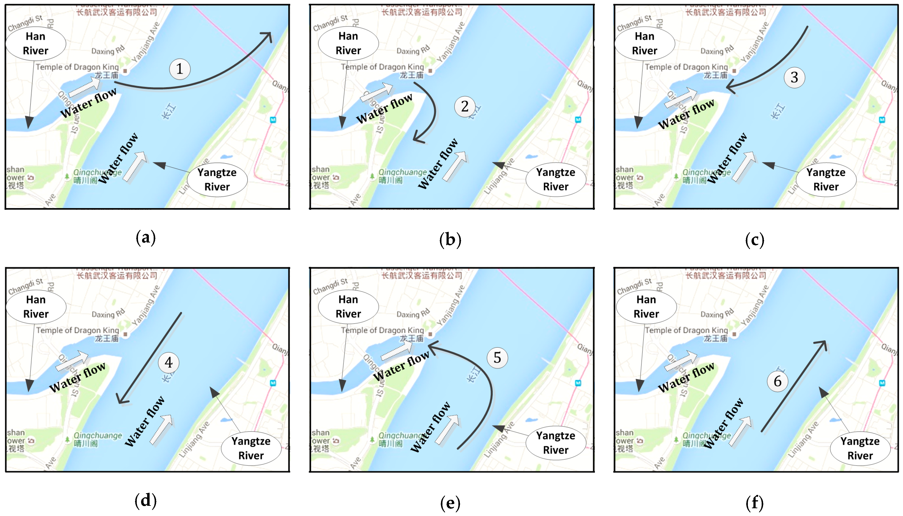
To validate the proposed methodology, a case study was conducted at Wuhan waterway, located at middle stream of Yangtze River, China. For the purpose of following the navigational rules and fuel prudent, captains tend to maneuver their vessels with a fixed pattern which make the SOG and COG of vessels in different routes characterized. The characteristic SOG and COG could be quantified by statistical analysis of dynamic AIS information. Take the marine traffic scene at the intersection waterway in Wuhan, China, for example. As shown in Figure 2, there are six directions of the traffic flow at the intersection waterway, which are labeled by number 1 to 6. For vessels in directions 4 and 6, the vessels will keep the speed and direction steady when they go through the channel of Yangtze River, hence the variance of SOG and COG would be small, and the mean of the COG would be similar to the direction of channel, what is more, for the rush of current, the mean of SOG in direction 4 will be lower than that in direction 6. For vessels in direction 1, i.e., voyaging downstream from Han River to Yangtze River, for the rush of current and turning direction, the mean of SOG should be higher than vessels in direction 3, and the variance of COG should be larger than vessels in directions 4 and 6. For vessels in direction 5, i.e., voyaging from upstream of Yangtze River to the Han River, due to the impact of current, the speed would decrease so that the variance of SOG gets larger, and the variance of COG also become larger. Similarly, other features can be found from the mean and variance of SOG, COG, respectively. In consequence, by statistical analysis of the four attributes of the vessels in different routes, the hidden motion pattern will be exposed, and can be transformed to pieces of evidence to make the inference.

The verified samples were acquired from Wuhan Maritime Administrator from 1 January 2014 to 31 August 2016. The samples from 1 January 2014 to 31 May 2014 (including 5486 verified samples) were applied to obtain the frequency distributions for the four attributes. The samples from 1 June 2014 to 31 October 2014 (including 3015 verified samples) were used to train the weight coefficient of evidence. The samples from 1 November 2015 to 31 August 2016 (including 17,723 samples in total) were invited to validate the accuracy of methodology proposed in Section 2.

3.1. Step 1: Statistical Analysis of the Attributes from Verified AIS Data

In order to extract the frequency distributions from historical AIS data, 220 samples for direction 1, 117 samples for direction 2, 244 samples for direction 3, 2260 samples for direction 4, 108 samples for direction 5, and 2537 samples for direction 6, were selected and analyzed.

• Attribute 1: Mean of SOG

When the accuracy of mean of SOG was set to 0.1, the frequency distributions of mean of SOG for six directions are shown in Figure 3.

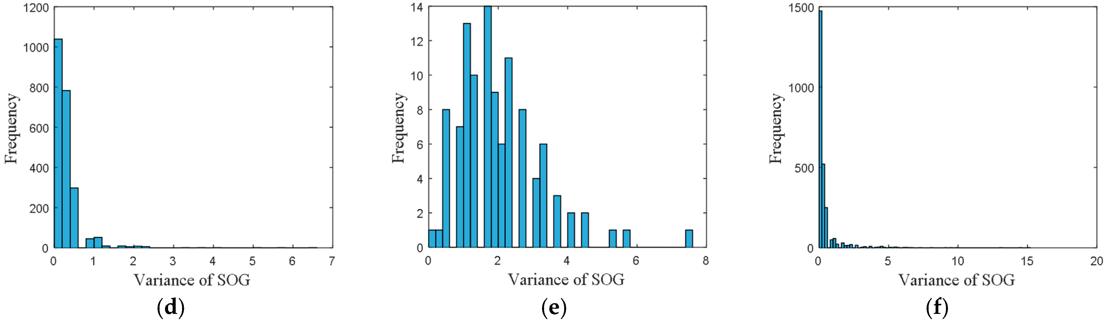
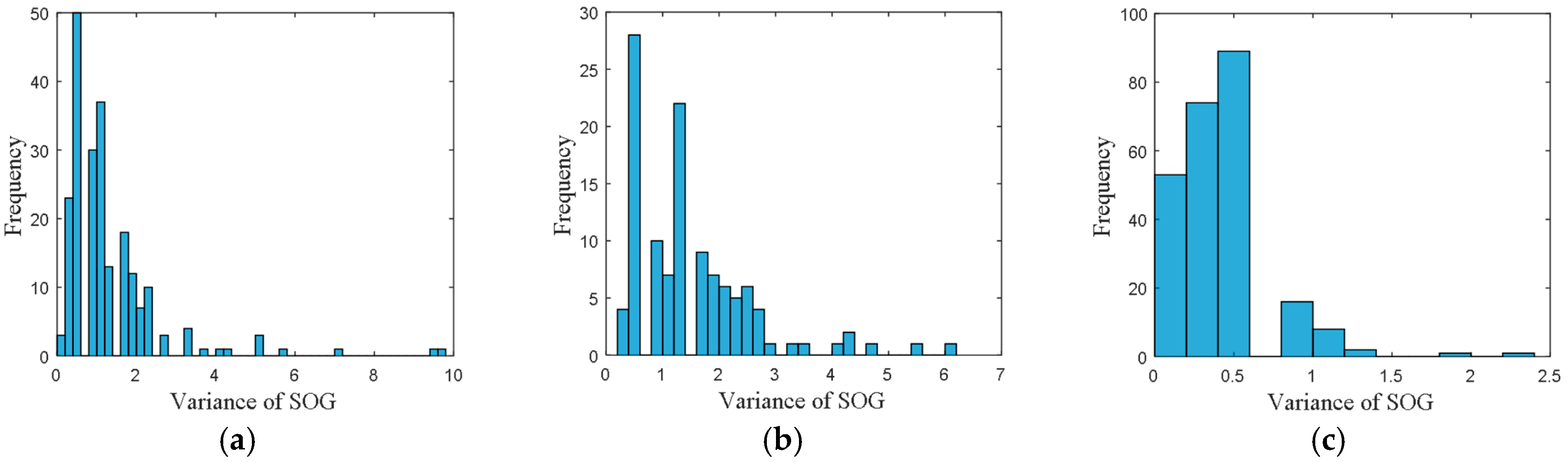
• Attribute 2: Variance of SOG

The frequency distribution of variance of SOG is shown in Figure 4, where the accuracy of variance of SOG was set to 0.2.

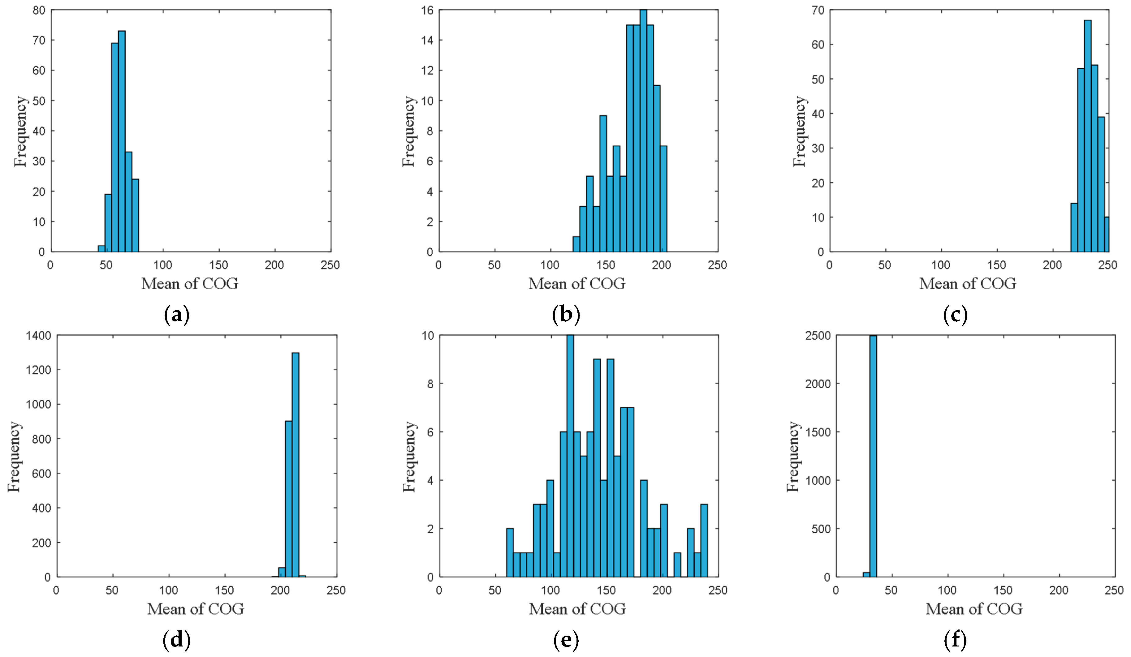
• Attribute 3: Mean of COG

The frequency distribution of mean of COG is shown in Figure 5, where the accuracy of the mean of COG was set to 6.

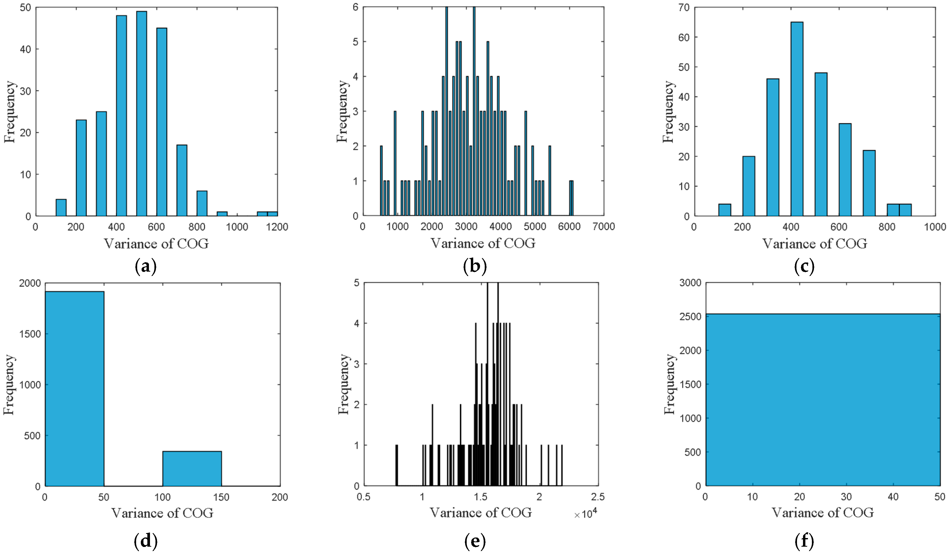
• Attribute 4: Variance of COG

The frequency distribution of variance of COG is shown in Figure 6, where the accuracy was set to 100.

From these frequency distributions, we found that the distributions are quite different for vessels in different directions. The differences of the distributions revealed the navigational pattern as the vessels voyaging along the routes.

3.2. Step 2: Belief Distribution by Likelihood

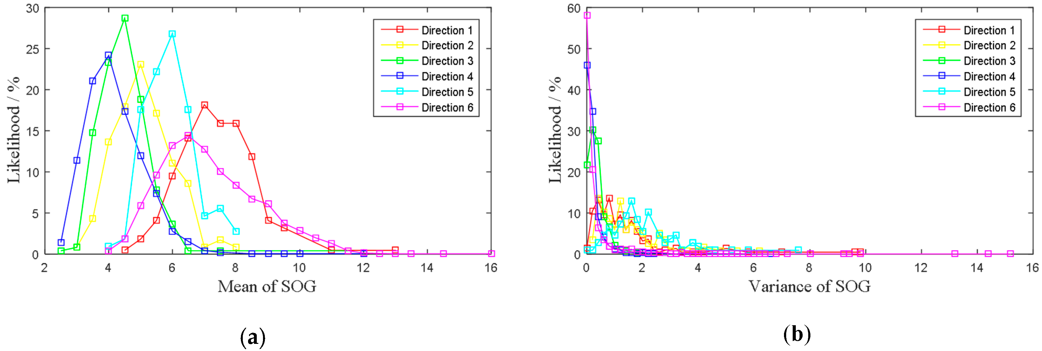
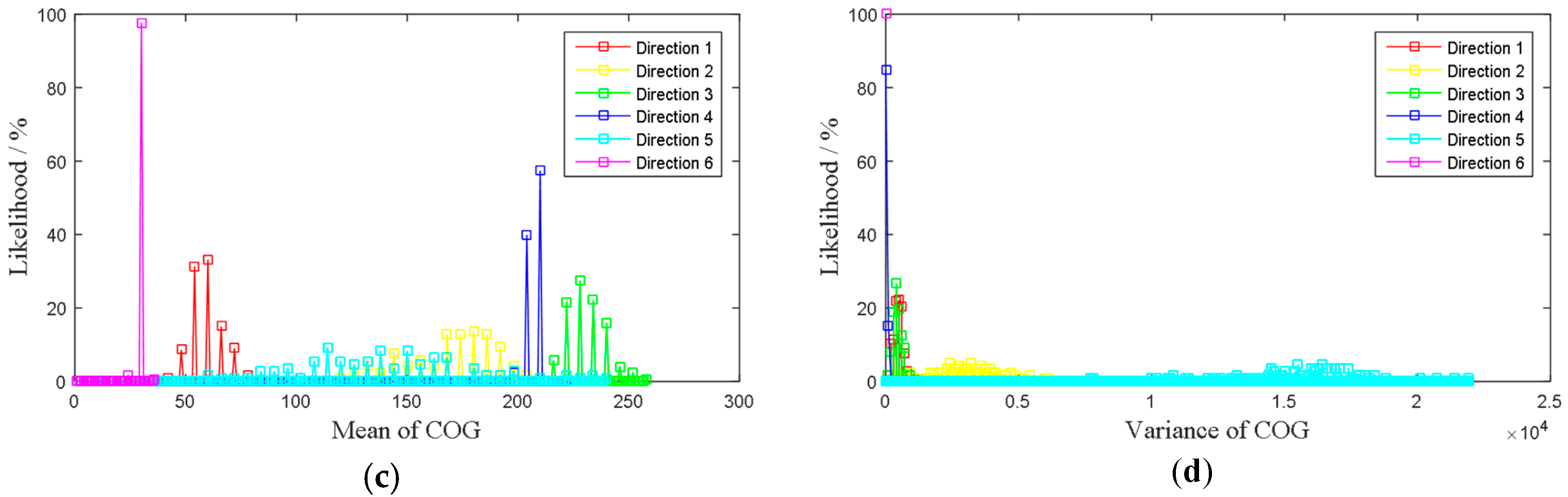
After obtaining the frequency distributions of mean and variance of SOG, COG for each direction, the following step is to find the probabilistic relationships between the distributing values and probabilities of each direction. According to the verified samples for each direction, the likelihoods can be obtained by Equations (2) and (3), with the four attributes distributions. Figure 7 shows the likelihoods distributions for each attribute.

Then, for any posterior AIS data cell, after calculating its four attributes value, the likelihoods of being in which direction can be obtained by Equations (2) and (3), with Figure 7. It is worthy to know that, if all the likelihoods of a posterior AIS data cell obtained from the figure are zero, which means that the verified sample failed to include all of the attributes. In consequence, the algorithm gives an ambiguous result, i.e., the result is unknown which direction it is. To solve this problem, more verified samples should be collected to form a perfect distribution. The suboptimal solution is to reform the distribution with Fitting functions.

3.3. Step 3: Evidence Combination

Through the procedures above, the correlation between the four attributes and the probabilities of vessels, being in which direction can be established, respectively. Then, with these correlations, the frequency distributions of AIS dynamic data can be mapped to pieces of evidence. Eventually, the ER rule is used to combine such evidence with different weights and reliabilities, which are conducted by Equations (6)–(9). As discussed, the reliability and weight coefficients of a piece of evidence that should be equal when there is no verified sample or a certain optimization objective [22]. All of the pieces of quantified evidence are from the AIS dynamic information, which originate from the GPS module. Liu et al. [25] shows that in Wuhan waterway, the error ratio of AIS messages is 27.56%. Since all of the dynamic information was originated from the AIS, the reliability coefficients for four attributes should be equivalent. In this research, all of the reliability coefficients were set to 0.7244. For all of the evidence, their reliability and weight coefficients should be equal in the first place, namely w^T = {w₁, w₂, w₃, w₄} = {0.7244, 0.7244, 0.7244, 0.7244}. Classification results of the verified samples with initial weight coefficient are presented in

Table 2. Classification results of the verified samples with initial weight coefficient.

Directions	Total	Correct Classification	Incorrect Classification	Accuracy
Direction 1	698	692	6	99.14%
Direction 2	812	758	54	93.35%
Direction 3	693	692	1	99.86%
Direction 4	6230	6220	10	99.84%
Direction 5	755	616	139	81.59%
Direction 6	8535	8535	0	100%
Overall	17,723	17,513	210	98.82%

.

Take the AIS data collected from 1 November 2015 to 31 August 2016 as the verified samples, the proposed methodology is validated as follows. Since there are six directions, the classification result should be the direction that the combined probability is largest. In other words, if the reasoning probability of a direction is larger than any other directions, this direction is considered as the final result. It should be mentioned that, if the reasoning probability of each direction is precisely equal, i.e., the classification is ambiguous, the judgment will be considered as a failure. The identification results are presented in Table 2.

From the result presents in Table 2, it can be seen that the developed model with initial weight coefficient produced 17,513 correct classifications out of 17,723 verified samples, leading to a classification accuracy of 98.82% overall.

3.4. Step 4: Non-Linear Optimization of Evidential Weights

Liu et al. [25] show that in Wuhan waterway, the error ratio of AIS messages is 27.56%. Since all of the dynamic information originated from the AIS, the reliability coefficients for four attributes should be equivalent. In this research, all of the reliability coefficients were set to 0.7244. In comparison, to obtain a proper weight coefficient of each piece of evidence is more complicated.

To make the classification more practical, appropriate weight coefficients [26,27,28] can be obtained with a certain objective and verified samples, as discussed in Step 4, Section 2. With the verified AIS data gathered from 1 June 2014 to 31 October 2014, including 106 samples for direction 1, 88 samples for direction 2, 116 samples for direction 3, 1151 samples for direction 4, 82 samples for direction 5, and 1472 samples for direction 6, weight coefficients can be trained based on the Equations (10) and (11).

Particularly, such a procedure can be implemented by the ‘fmincon’ function of MATLAB2015a. This procedure will consume a certain amount of time, and more appropriate weights are solved as w^T* = {w₁, w₂, w₃, w₄} = {0.45, 0.45, 0.45, 0.55}. In this occasion, w^T* is used as the weight vector for the verified samples. The obtained results are presented in

Table 3. Classification results of the verified samples with optimized weight coefficient

Directions	Total	Correct Classification	Incorrect Classification	Accuracy
Direction 1	698	691	7	99%
Direction 2	812	772	40	95.07%
Direction 3	693	692	1	99.86%
Direction 4	6230	6221	9	99.86%
Direction 5	755	623	132	82.52%
Direction 6	8535	8535	0	100%
Overall	17,723	17,534	189	98.93%

.

Compare the results with Table 2, after training the weight coefficient under the constraint of minimum global deviation, the number of incorrect classification decreased by twenty-one, and the overall accuracy raised a little. In fact, other optimization objectives can be taken into consideration, for example, the higher accuracy for vessels in direction 1. The optimization objective depends on the practical needs for the classification of AIS data.

4. Conclusions

This paper proposed an ER rule-based methodology to build the artificial intelligence, which imitates the maritime administrators to classify and extract data from AIS database.

Using likelihoods to establish the mapping functions between frequency distributions and the support degree of evidence is feasible. The likelihood modelling can effectively transform the frequency distributions into pieces of evidence even if the number of samples in different categories is unbalanced.

The ER rule is more rigorous and reasonable than Dempster’s rule, because it takes the reliability and weight of evidence into consideration, which is more accord with the intelligence of human beings. Moreover, the ER rule resolved the paradox in DS theory.

The optimization of the weight coefficient can raise the classification accuracy, but it depends on the quantity and quality of validated samples. It should be mentioned that, if the ER rule with the initial weight coefficient could give high classification accuracy, the optimization of the weight coefficient would be a futile effort.

In the case study, with multiple pieces of evidence extracted from verified AIS data and the ER rule, the classification accuracy for each direction is on a quite high level.

In this paper, the proposed methodology is comprised of four steps, respectively, are attributes extraction, evidence modeling by likelihood, evidential combination by ER rule, and weights optimization with verified samples. To illustrate the methodology, we gave a case study on routes extraction at an intersection waterway, Wuhan, China. The proposed methodology can also be applied in other circumstances, such as routes classification in port areas.