Article

Arsenic Adsorption onto Minerals: Connecting Experimental Observations with Density Functional Theory Calculations

1
Department of Geosciences, The Pennsylvania State University, University Park, PA 16802, USA
2
Division of Science, The Pennsylvania State University, Berks, Reading, PA 19610, USA
3
Earth and Environmental Systems Institute, The Pennsylvania State University, University Park, PA 16802, USA
*
Authors to whom correspondence should be addressed.
Minerals 2014, 4(2), 208-240; https://doi.org/10.3390/min4020208
Submission received: 24 December 2013 / Revised: 25 February 2014 / Accepted: 6 March 2014 / Published: 27 March 2014
(This article belongs to the Special Issue Advances in Low-temperature Computational Mineralogy)

Abstract

:
A review of the literature about calculating the adsorption properties of arsenic onto mineral models using density functional theory (DFT) is presented. Furthermore, this work presents DFT results that show the effect of model charge, hydration, oxidation state, and DFT method on the structures and adsorption energies for AsIII and AsV onto Fe3+-(oxyhydr)oxide cluster models. Calculated interatomic distances from periodic planewave and cluster-model DFT are compared with experimental data for AsIII and AsV adsorbed to Fe3+-(oxyhydr)oxide models. In addition, reaction rates for the adsorption of AsV on α-FeOOH (goethite) (010) and Fe3+ (oxyhydr)oxide cluster models were calculated using planewave and cluster-model DFT methods.

Graphical Abstract

1. Introduction

1.1. Arsenic Chemistry, Geochemistry, Prevalence, and Toxicity

The study of arsenic (As) adsorption on mineral surfaces is necessary to understand both the distribution and mobility of As species in nature as well as to develop remediation strategies for As waste sites. Arsenic is found in a variety of geochemical environments at aqueous concentrations varying from <0.5 to >5000 μg/L, and is found in a variety of geochemical environments [1,2]. Natural and anthropogenically-mediated biogeochemical interactions among arsenic species, biota, and minerals can affect the distribution, mobility, and toxicity of As in the environment [2,3,4,5,6,7,8]. Although recent work has posited that arsenic could be a potential biochemical and astrobiological proxy for phosphorus during biological evolution [9], this hypothesis is controversial [10].
Arsenic can occur in both inorganic (iAs) and organic (oAs) forms; the chemical form of As, or species, as well as the concentration of As, affects the solubility, mobility, reactivity, bioavailability, and toxicity of As [11,12]. iAs occurs predominately as either arsenious acid (HnAsIIIO3n−3; sometimes called arsenous acid) in reducing environments, or arsenic acid (HnAsVO4n−3) in oxidizing environments, where n = 0, 1, 2, or 3 [12,13,14]. Both the oxidation and protonation states of iAs depend on the physiochemical conditions of the sample environment [2]. For example, the three pKa values for arsenic acid are 2.2., 6.9, and 11.5 [15]; therefore, the pH of the environment will affect the protonation state of H3AsO4, which will, in turn, affect the mobility, reactivity, and bioavailability of iAsV. In addition to iAs, methylated AsIII and AsV compounds such as monoarsinic acid (MMAV) and dimethylarsinic acid (DMAV) occur both naturally and due to anthropogenic sources [12,13]. Arsenic toxicity depends on the species present; a general trend of decreasing toxicity is: R3As > H3AsO3 > H3AsO4 > R4As+ > As0, where R is an alkyl group or a proton [12,16].
Arsenic originating from natural water-rock interactions of surface and groundwater [2,6] and from anthropogenic sources such as acid mine drainages [17,18] can lead to drinking water contamination. Biogeochemical processes result in organic As compounds accumulating in oil, shale, and coal [19]. DMA and MMA have been used as herbicides, pesticides, and defoliants and pose a contamination problem to surface and groundwater [20]. Roxarsone (C6AsNH6O6) is used as a supplement in chicken feed and ends up in waste from poultry operations [21]. In addition to natural and anthropogenic groundwater contamination by As, anthropogenic As is contaminating the oceans, and subsequently seafood [16], which could have human health implications.
Human diseases caused by As contamination include various cancers, liver disease, cardiovascular disease, and an increase in mortality from pulmonary tuberculosis [22,23,24,25,26,27,28]. Groundwater that contains As concentrations >10 μg/L limit set by the World Health Organization (WHO) places more than ten million people at risk from arsenicosis. Locales ranging from Southern Bangladesh, India, Argentina, Chile, and Vietnam have groundwater sources with As concentrations >10 μg/L [2,3,6,25,26,28,29,30,31,32,33].
The remediation of arsenic in aquifers can be challenging due to the size of contaminated groundwater systems and varying biogeochemical conditions. For instance, the shallow groundwater of the Chaco Pampean Plain of Argentina spans 106 km2 and contains 10 to 5300 μg As/L [34]. A variety of As remediation methods were reviewed recently [35,36]; these methods have shown varying success rates. For example, an in situ study of an alkaline aquifer showed relatively low adsorption of iAs [37]. Conversely, a permeable reactive barrier study showed As removal to <5 μg/L due to induced sulfate reduction and the presence of zero-valent Fe [38], and experiments with household sand filters in Vietnam were able to reduce As concentrations in drinking water to <10 μg/L with a 40% success rate [39]. Laboratory and field experiments with household zero-valent Fe filters showed similarly effective results in Bangladesh [40]. Field tests with Fe-coated zeolites showed 99% removal of As [41]. Mn-Fe oxide-coated diatomites were able to reduce iAs from >40 μg/L to <10 μg/L in a pilot field-scale study [42]. Although many of these studies show promise for field-scale remediation of As, the biogeochemistry, aqueous geochemistry, and mineralogy of the surface and groundwater can affect the efficiency of the methods; therefore, it is necessary to understand the As adsorption process more thoroughly, so that the remediation methods can be applied more effectively.

1.2. Arsenic Treatment Methods

Due to the prevalence of As contamination worldwide and the threat of arsenicosis [43], research and the development of methods to understand As chemistry and to attenuate As in water are imperative [44]. Methods that have been developed to attenuate As such as electrocoagulation and electrodialysis [45,46], treatment with microorganisms to affect the biogeochemical cycling of As [7], and the adsorption of As onto a variety sorbents [47,48,49]. Among the sorbents used for As attenuation are organic polymers [50], and minerals such as dolomite [51], zeolites [52], and Al minerals such as alumina or gibbsite [53,54]. Alumina has been found to effectively remove iAsV [55], but it is necessary to use activated alumina to efficiently remove iAsIII from solution [56]. A multitude of studies on As adsorbents have been conducted using Fe-based mineral sorbents [57,58], such as magnetite [54,59,60,61,62,63], ferrihydrite [53,54,64,65,66], goethite [48,54,66,67], and zero-valent iron [62].
The focus of the current work is on the chemistry of iAs species adsorbed to Fe-oxide and Fe-hydroxide mineral surfaces. Prior experiments have found that inorganic [64] and organic [64,68,69,70] ligands may adsorb to Fe minerals and compete with As for adsorption sites, but Zn cations [59] may augment As adsorption to Fe sorbents. Therefore, if ligands that inhibit As adsorption can be removed or precipitated and ligands that enhance As adsorption can be added to As-containing site, it could be possible to develop improved As-remediation techniques. Arsenic adsorption may also be enhanced by the addition of magnetite to agricultural waste such as wheat straw [61], but adsorption of As can be reduced by microorganisms [7,66]. If it is possible to control the growth and metabolism of microorganisms present in As-containing water, then it could be possible to enhance As adsorption.

1.3. Studying As Adsorption with Experimental and Modeling Methods

Because of the complex and often uncharacterized biogeochemistry of arsenic-rich environments, it is useful and necessary to use a variety of experimental data and modeling results to characterize these complex matrices. For example, Figure 1 shows models of the monodentate, bidentate, and outer-sphere adsorption of HAsO42− to Fe-(oxyhyr)oxide clusters (Figure 2A–C) and periodic models (Figure 2D–F) models. Experimental and modeling techniques have been employed to determine the geometries, energetics, and spectroscopic properties exhibited by As species adsorbed to mineral surfaces; improved knowledge about the adsorption chemistry of As species can aid in the development of methods for attenuating As in the environment. Although the focus of our work is on the use of quantum mechanics (QM) techniques for studying the properties of As adsorption, it is necessary to frame these results in relationship to experimental and other modeling methods, because QM results can be useful for interpreting experimental data and for parameterizing other modeling methods such as classical force fields [71] and surface complexation models [72,73].
Figure 1. (A) Ferric iron (oxyhydr)oxide cluster model of Fe2(OH)6(H2O)4·4H2O; (B) monodentate mononuclear (MM) cluster model of Fe2(OH)5(H2O)4H2AsO4·4H2O; and (C) binuclear bidentate (BB) cluster model of Fe2(OH)4(H2O)4HAsO4·4H2O.
Minerals 04 00208 g001
Figure 2. (A) and (D) monodentate mononuclear adsorption of HAsO42−; (B) and (E) bidentate binuclear adsorption of HAsO42−; and (C) and (F) outer-sphere complex of HAsO4, on clusters of Fe3+-(oxyhydr)oxide (AC) and periodic α-goethite (010) (DF) models.
Minerals 04 00208 g002

1.4. Studying As Adsorption with Experiments

Vibrational spectroscopy (e.g., Fourier transform infrared spectroscopy (FTIR) or Raman), X-ray absorption near edge structure (XANES), extended X-ray adsorption fine structure (EXAFS) spectroscopies, as well as adsorption isotherm and kinetics experiments are useful for determining the chemistry of As adsorption. FTIR and Raman studies are useful for determining the bonding configurations between As species and mineral surfaces. When As adsorbs as an inner-sphere complex, characteristic vibrational frequency shifts are observable [74,75,76,77,78,79]. XANES spectroscopy can provide information about the oxidation state of As that is adsorbed to mineral surfaces [80,81,82,83,84], and can determine if the oxidation state of As or the surface changes during the adsorption process [78,85]. EXAFS spectroscopy provides information about the coordination chemistry of adsorbed As [46,80,81,82,86,87,88,89,90,91,92]. Coordination state information is useful for determining whether the As adsorbs as a monodentate, bidentate, or outer-sphere complex (Figure 2). Moreover, studies that use two or more instrumental methods such as XANES/FTIR [78] or XANES/EXAFS [82] can increase the reliability of data interpretation. Furthermore, kinetics and isotherm studies provide information about the rates and energetics of As adsorption onto mineral surfaces that further help constrain adsorption mechanisms [55,93,94,95,96,97].
Although experimental techniques have contributed greatly to the understanding of As adsorption chemistry, computational chemistry can be used to help interpret experimental data on the mechanisms of As adsorption to mineral surfaces. In addition, computational chemistry can fill in missing information on the details of adsorption mechanisms and kinetics.

1.5. Studying As Adsorption with Mathematical Models

Surface complexation modeling (SCM) techniques such as the charge distribution multi-site complexation (CD-MUSIC) [76,95,98,99,100,101,102,103,104,105,106], the extended triple-layer model [107], isotherm modeling [108,109], and the ligand and charge distribution model (LCD) [110,111] have been used to model As species in solution and adsorbed to mineral surfaces. In general, SCM models use experimental data or quantum mechanics results such as equilibrium constants, bond lengths, and surface charges to calculate the adsorption isotherms of As on Fe mineral surfaces. When integrated, the CD-MUSIC and LCD SCMs are able to model humic substances interacting with Fe surfaces and the effect they have on As adsorption [111,112]. SCM can be used to interpret interactions among As, mineral surfaces, and organic and inorganic ligands, as well as charge and protonation effects. However, the precision of these models depends on the quality of their parameterization that is obtained from experimental data, which can be difficult to interpret, or with QM results [72,73].

1.6. Studying As Adsorption with Quantum Mechanics Modeling Methods

Numerous studies applying QM, or specifically density functional theory (DFT) methods [113,114], use models similar to those shown in Figure 2A–C. For example, DFT methods have been used to study the thermodynamics [91,115,116,117], vibrational frequencies [75,118,119,120,121], kinetics [120,121,122], ligand effects [87], oxidation-reduction reactions [123], and the coordination of adsorbed As [90,91,117,119,124,125,126,127,128,129,130,131,132].
Many of the previous computational chemistry studies relied on cluster models such as those in Figure 2A–C, but some groups have used periodic models to capture the chemistry of the mineral surface sorbates more precisely [124,125,127]. In this paper, we report structures and kinetics comparisons for the results from both cluster models (Figure 2A–C) and periodic models (Figure 2D–F). These comparisons are necessary to determine if and how the results from the molecular cluster and periodic model calculations differ.
In addition to the use of cluster versus periodic models, other factors can affect the results obtained from DFT calculations. These factors include surface charge, hydration, model convergence criteria, and potentially the software used for the calculation. For example, prior studies used highly charged models [91] to study the adsorption of As to Fe clusters; however, the work that we are presenting used models for the surface clusters with neutral charges, because localized high charges are unlikely. Prior work using the implicit solvation using the conductor reaction field (COSMO) [133,134] suggests that a single water molecule can produce activation energy results that are more precise than the addition of multiple water molecules can [122]. Conversely, other studies have used anhydrous surfaces to model As adsorption to Fe clusters [91]. The work we present herein used both hydrated cluster models and hydrated periodic models in an attempt to model the natural environment of As adsorption more accurately and realistically.
As the processing power and speed of computers increases, the size and complexity of As adsorption models increases, as illustrated by two Fe cluster models from papers dating from 2001 and 2006 [90,129]. The Fe cluster model in the latter paper is larger and likely more realistic than the model in the former paper. Results from prior DFT calculations provide contradictory results about the coordination state of As adsorption. For example, there are DFT results that predict that monodentate [128], bidentate [90,91,119,129], or a mixture of As coordination states are occurring on Fe-mineral surface models [130]. Because both the experimental data and the DFT results are providing ambiguous information about As coordination state, further calculations and experiments are necessary to clarify this topic. Alternatively, As may adsorb in a variety of configurations depending upon which surfaces are present on a given mineral sample [135].
The convergence criteria of the energy minimization calculations for the models could also have an effect on the precision of the calculated results and the ability of the results to reproduce experimental data and provide insight about As adsorption chemistry. For example we use a minimization convergence criteria of 0.03 kJ/mol, whereas, for example, Sherman and Randall [91] used higher tolerance energy minimization criteria 5 kJ/mol; however, tighter convergence criteria again reflects the availability and evolution of computational resources.
In the studies presented here, the thermodynamics, geometries, and kinetics of inner-sphere iAsIII and iAsV adsorbed as monodentate mononuclear (MM) or bidentate binuclear (BB) complexes to solvated Fe clusters were evaluated. The molecular cluster results show how hydration and the initial Fe cluster charge affect iAsIII and iAsV adsorption for BB models, and the results compare the of adsorption energies of BB iAsIII and iAsV onto hydrated neutral Fe clusters. The DFT calculations on the cluster models also compare the calculated As—Fe distances for the BB models with pertinent experimental observations. In addition, inner- and outer-sphere As-Fe complexes were used to determine the activation energies (ΔEa) of the adsorption/desorption process; these calculations were performed using both molecular cluster models and periodic models of the α-FeOOH (goethite) (010) surface.

2. Methods

2.1. Applied Quantum Mechanics Background

The application of QM with quantum chemistry software allows one to calculate chemical properties such as thermodynamics, kinetics, molecular geometries, spectroscopic parameters, transition states structures that might not be experimentally observable, and potentially hazardous chemistries [136,137,138].
Quantum chemistry calculations begin with an initial input of Cartesian coordinates for the molecule of interest, and then these coordinates are subsequently allowed to change during energy minimization calculations. The bond lengths, bond angles, and dihedral angles of the model are systematically perturbed, followed by the calculation of the relative energy of the model. After each energy calculation, subsequent systematic perturbations of the model geometry take place until the force (F), where F = dE/dr and dE and dr are the change in the energy and change in the model coordinates, respectively, converges to at or near “zero” (i.e., “zero” is defined as the convergence criteria by the modeler). When F is zero, the model then resides at a stationary point on a potential energy surface (PES). The user of computational chemistry software can specify the criterion for energy minimization convergence [136,139].
Subsequent calculation of the vibrational frequencies for the model determines the second derivative of energy with respect to atomic coordinates (d2E/dr2). If the calculated vibrational frequencies are all real (positive), then the model is at a PES minimum; if one vibrational frequency is imaginary (negative), then the model is at a transition state or PES maximum; if the model exhibits > 1 imaginary frequency, then the model is unstable and a new input geometry should be used. Obtaining a PES minimum does not guarantee that the model is at a global minimum, only that the model is at a local minimum. Using multiple input models obtained from a conformational analysis can aid in the attainment of a globally minimized final geometry [136,139].
The calculation of the vibrational frequencies (d2E/dr2) also allows the calculation of thermodynamic properties such as enthalpy, Gibbs free energy, and entropy. If one imaginary frequency is present, the model is at a transition state and the results from this model, the initial structure of the model, and the PES minimum model can be used to calculate rate constants for reactions. Note that throughout the manuscript the output from QM calculations is referred to as results and not data, we refer to the output from experiments as data. The vibrational frequency calculation provides infrared and Raman frequencies for the model, and further calculations can provide NMR chemical shifts, UV-Visible wavelengths, isotope effects, and temperature effects [136].
There are numerous methods available for calculating energies and other chemical properties with QM, among the most widely used are Hartree-Fock (HF) method [140], Møller-Plesset perturbation (MP) theory [141], and density functional theory (DFT) [113,114]. All of these methods arose from the development of quantum mechanics and the Schrödinger equation (ĤΨ(r) = EΨ(r)), where Ĥ is a Hamiltonian operator, Ψ(r) is the wave function, and E is the energy of the model. If Ψ(r) is known for a model, it is possible to solve for E and thus obtain the molecular properties for any model of interest. The Schrödinger equation has only to solve for the electronic energy of the model, because the nuclear energy and positions are relatively low and stationary compared to those of the electrons [142]. Thus far, it has been impossible to solve the Schrödinger equation for models that are more complex than H2 because Ψ(r) makes the solution of the equation untenable for larger molecules with a greater number of electrons; therefore, it has been necessary to develop approximations for the Schrödinger equation such as HF and MP theory.
HF theory minimizes the energy of each electron iteratively with respect to the average energy of the other electrons in a model [140]. The shortcoming HF is that it does not account for electron correlation (repulsion) between each electron in the model. Using HF leads to an overestimation of model stability. MP theory accounts for electron correlation by systematically perturbing the molecular Hamiltonian [141]; however, the cost of using MP theory is prohibitive for models of geochemical interest. Furthermore, unlike HF theory, MP theory is not variational [143], so, the calculated energy could be lower than the ground state energy.
Unlike HF and MP theories that calculate electron interaction to obtain molecular energies, DFT calculates the electron density of the molecule to determine the energy [113,114,144]. The shortcoming of DFT is that the theory lacks a method for calculating the exact energy of the electron correlation and exchange term (Exc). The inability to calculate the Exc results in an underestimation of the total energy. Neglecting Exc, as HF theory does, or underestimating Exc, as DFT does, results in an underestimation of the total energy of a given model. For DFT, the lack of a precise correlation energy results because DFT does not account for the columbic interaction (repulsion) between electrons with anti-parallel (opposite) spin. Imprecise exchange energy results because DFT does not account precisely for the fact that electrons with parallel (same) spins cannot reside in the same orbital. Therefore, neglecting or underestimating the Exc violates the Pauli Exclusion Principle. However, a variety of DFT methods have been developed to approximate Exc and these methods can produce precise results [138,145]. Significantly, the computational cost of DFT calculations is substantially less than the cost of MP theory calculations, and the precision of DFT calculations is greater than that of HF calculations. Therefore, although DFT methods account imprecisely for Exc, they are preferable to HF and MP methods.
Many DFT methods are available, and a particular method could be useful for calculating a particular chemical property (e.g., energy) but not for calculating other properties (e.g., NMR chemical shifts); these differences in precision are due to the parameters used for Exc in the DFT methods [138,145]. Additional work is necessary to evaluate the efficacy of DFT methods for calculating properties such as adsorption energies, rate constants, and structures. Although DFT methods such as B3LYP [146,147] can provide accurate results for a variety of chemical properties, we suggest that computational geochemists begin to explore the use of other DFT methods that could provide improved results.
In addition to using an electron correlation method such as MP or DFT, it is necessary to specify a basis set when using molecular orbital (MO) calculations [136,148,149,150,151]; however, when using planewave calculations [152,153,154,155,156,157,158], basis sets are not used.
For DFT calculations on the clusters, the basis sets are equations that define atomic orbitals and are used in linear combinations to create molecular orbitals. When using basis sets, each atomic orbital for a given atom contains one electron [149], so for the C atom, which has six electrons and an electronic configuration of 1s22s22p2, it is necessary to have a minimum of five basis functions (i.e., 1s, 2s, 2px, 2py, and 2pz). Note that because the p-orbitals are energetically degenerate, the 2px, 2py, and 2pz are present as basis functions. The variational principle of quantum mechanics states that Eg ≤ ⟨Ψ(r)∣Ĥ∣Ψ(r)⟩, where Eg is the ground state (lowest) energy of the molecule. The variational principle shows that increasing the accuracy of Ψ(r) will increase the calculated accuracy E relative to Eg; increased basis set size can increase the accuracy of Ψ(r).
Basis set size can be increased by using double zeta (DZ) or triple zeta (TZ) basis sets which double or triple the number of basis sets used, relative to the minimal basis set [148]. For C, the DZ and TZ basis sets have ten and fifteen basis functions, respectively. Another method for increasing the accuracy of a basis set is to use split basis sets, where more basis sets are used for the bond-forming valence electrons, while the non-bond-forming core electrons are treated with minimal basis sets. For C, this would involve one 1s orbital and two each of the 2s, 2px, 2py, and 2pz basis sets for a total of nine basis sets.
Further increases in basis set size and precision can be obtained by the addition of polarization and diffuse basis functions [148]. Polarization functions increase the angular momentum basis sets on a particular atomic orbital; for example, in methane each H atom has a 1s orbital, but in the C-H bonds, the H atoms receives some p-orbital character from the C atom; therefore, including p-orbital polarized functions on the H atoms increases the accuracy of the orbital description. In addition, diffuse basis sets are used increase the electronic radius where electrons can reside. Diffuse basis sets are useful for calculations with anions and for weak interactions such as van der Waals interactions.

2.2. Molecular Orbital Theory Calculations with Fe Clusters

For the cluster model DFT calculations, all models were constructed in Materials Studio (Accelrys Inc., San Diego, CA, USA) and the energy minimization, Gibbs free energy, and transition-state calculations were performed in the gas phase using Gaussian 09 software [136]. All energy minimization calculations on the cluster models were performed without symmetry or atomic constraints. Energy minimizations, frequency, and kinetics (transition state) calculations were performed using the hybrid density functional B3LYP with the 6-31G(d) basis set [148,149,150,151]. B3LYP accounts for Exc and the 6-31G(d) basis set is a DZ basis set with p-polarization functions on the non-H atoms. Energy convergence was set to 0.03 kJ/mol during the energy minimization calculations. The frequency calculations using B3LYP/6-31G(d) ensured that each model was at either a potential energy minimum (no imaginary frequencies) or at a transition state (one imaginary frequency) [136]; however, the frequency calculation does not ensure the model is at a global energy minimum.
For Gaussian calculations, it is necessary to specify an electron correlation method (e.g., B3LYP), a basis set, the type of calculation (e.g., optimization), the Cartesian coordinates of the atoms in the model, the charge of the model, and the spin multiplicity of the model [136]. The electron configuration of Fe3+ is [Ar]3d5. For the energy minimization calculations, we used high-spin Fe3+, where each 3d electron occupies one of the five d-orbitals, and where the electrons are all either spin up or spin down; this means that each of the two Fe atoms in the cluster has five unpaired electrons. The multiplicity is = 2S + 1, where S is the spin of an unpaired electron and can be +½ or –½. Therefore, for our high-spin clusters there are 10 unpaired electrons, each having a spin of +½, so the multiplicity = 2(10/2) + 1 or 11. For the rate constant calculations, we experimented by using high-spin multiplicity for both Fe atoms (i.e., 11), and a combination of up spin for one Fe atoms (i.e., +5) and down spin for the other (i.e., −5).
Fe model surface complex clusters were designed to minimize surface charge because charge buildup on the actual mineral surfaces is believed to be relatively small. However, surface models with charges were also calculated to demonstrate the effect of model charge on calculated energetics, and to compare with prior studies that used charged models [91]. In addition, explicit hydrating H2O molecules were included for the aqueous species, the surface Fe-OH groups, and the adsorbed arsenic acid (iAsV) molecules. Figure 1 shows examples of a tetrahydrated Fe (oxyhydr)oxide cluster, (Fe2(OH)6(H2O)4, A, without adsorbed HAsO42−, B, monodentate mononuclear (MM) adsorbed HAsO42−, and C, bidentate binuclear (BB) adsorbed HAsO42−. Hydration can be a key in accurately predicting structures and frequencies of anionic surface complexes because they are both a function of the hydration state of the sample [75,157]. The interatomic distances calculated in each model surface complex were compared to As-O bond lengths and As—Fe distances obtained from EXAFS spectra [46,80,81,82,86,87,88,89,90,91,92].
Gibbs free energies (G) of each species were estimated by calculating G in a polarized continuum the permittivity for water of 78.4 at 298.15 K. The integral equation formalism of the polarized continuum model (IEFPCM) [159] was used to calculate the Gibbs free energy in solution. The polarized continuum places the model in the cavity of a field with a constant permittivity, in this case for water; this field is used as a proxy for the solvent of interest. Single-point energy calculations were performed with the B3LYP functional and the 6-31+G(d,p) basis set [148,149,150,151]; the TZ basis set with augmented functions on the non-H atoms, and d-polarized and p-polarized functions for the non-H atoms and H-atoms, respectively, was used in order to improve the accuracy of the energy that was calculated using B3LYP/6-31(d) during the energy minimizations; this is a standard practice. The ΔGads was then determined from stoichiometrically balanced reactions. Configurational entropy terms are neglected in this approach; hence, we emphasize that these are Gibbs free energy estimates. We do not expect the precision of ΔGads to be better than ±10 kJ/mol.
To illustrate the potential effect that a chosen DFT method can have on geometry and thermodynamics, we report the As—Fe, As-OH, As=O, and As-OFe bond distances for the Fe2(OH)4(OH2)4HAsO4·4H2O model and ΔGads for the reaction:
H2AsO4·8H2O + Fe2(OH)6(OH2)4·8H2O → Fe2(OH)4(OH2)4HAsO4·4H2O + OH·4H2O + 5H2O
For this reaction, we used either B3LYP, PBE0 [160,161,162], and M06-L [163] DFT methods to minimize each structure in the reaction with the 6-31G(d) basis set, and the 6-311+G(d,p) basis with the self-consistent reaction field (SCRF) IEFPCM and the solvent water to calculate the single-point energy of each structure. The PBE0 and M06-L methods were chosen to compare with the results from the often-used B3LYP method, because the PBE0 function was the method used for the periodic planewave calculations for this work, and the M06-L method was specifically parameterized for use with transition metals such as Fe [162].
For the transition-state calculations on the clusters, the outer-sphere complexes of AsO43− on an Fe3+-(oxyhydr)oxide clusters were obtained by constraining one Fe—As distance and allowing all other atoms to relax. The constrained distance was increased incrementally, allowing for energy minimization of the system at each new distance. The reaction path was graphically visualized. The change in energy for the adsorption reactions (ΔEads) were inferred by using the total electronic energy plus the zero-point correction obtained from the inner-sphere frequency calculations [163].

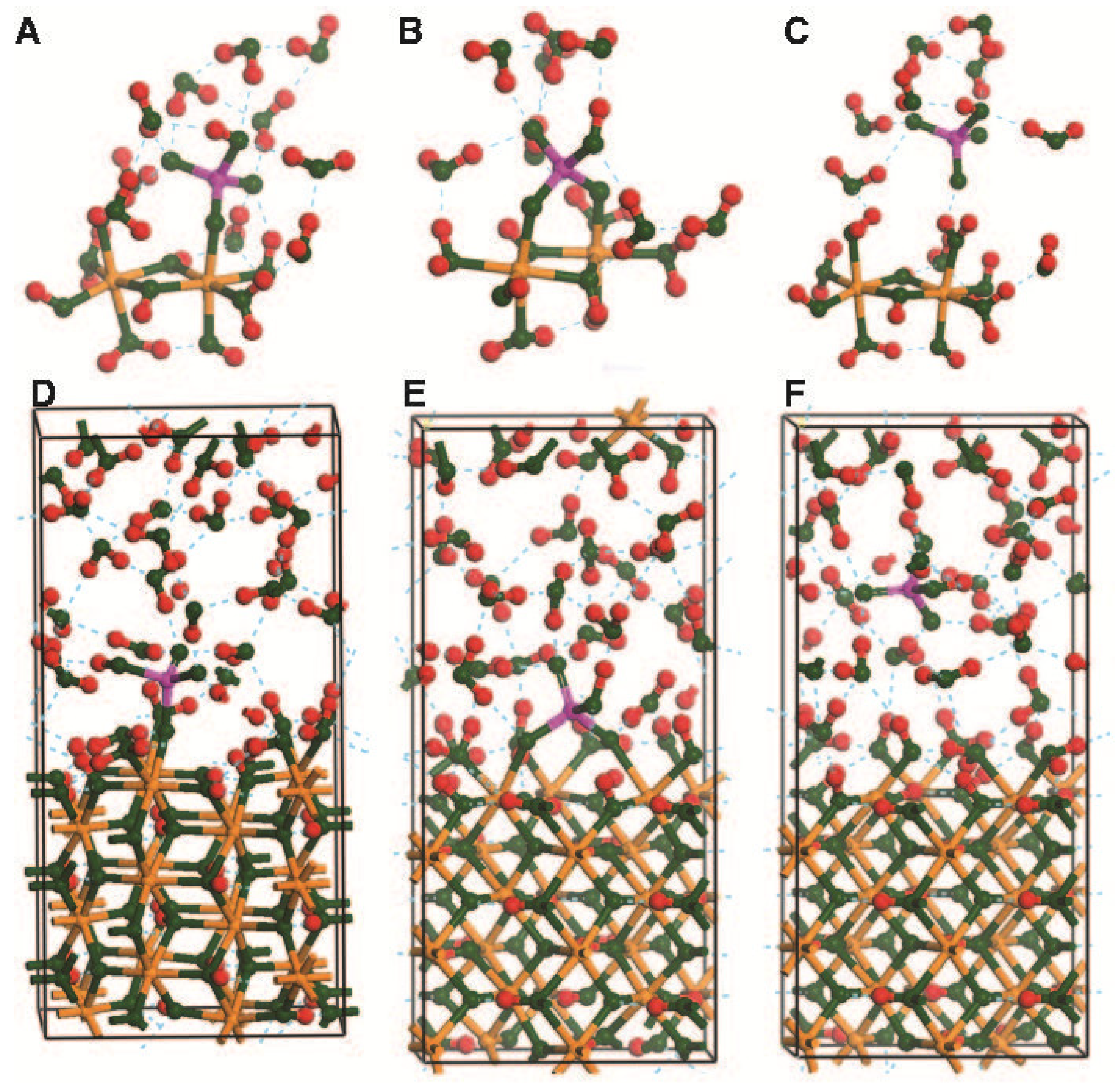
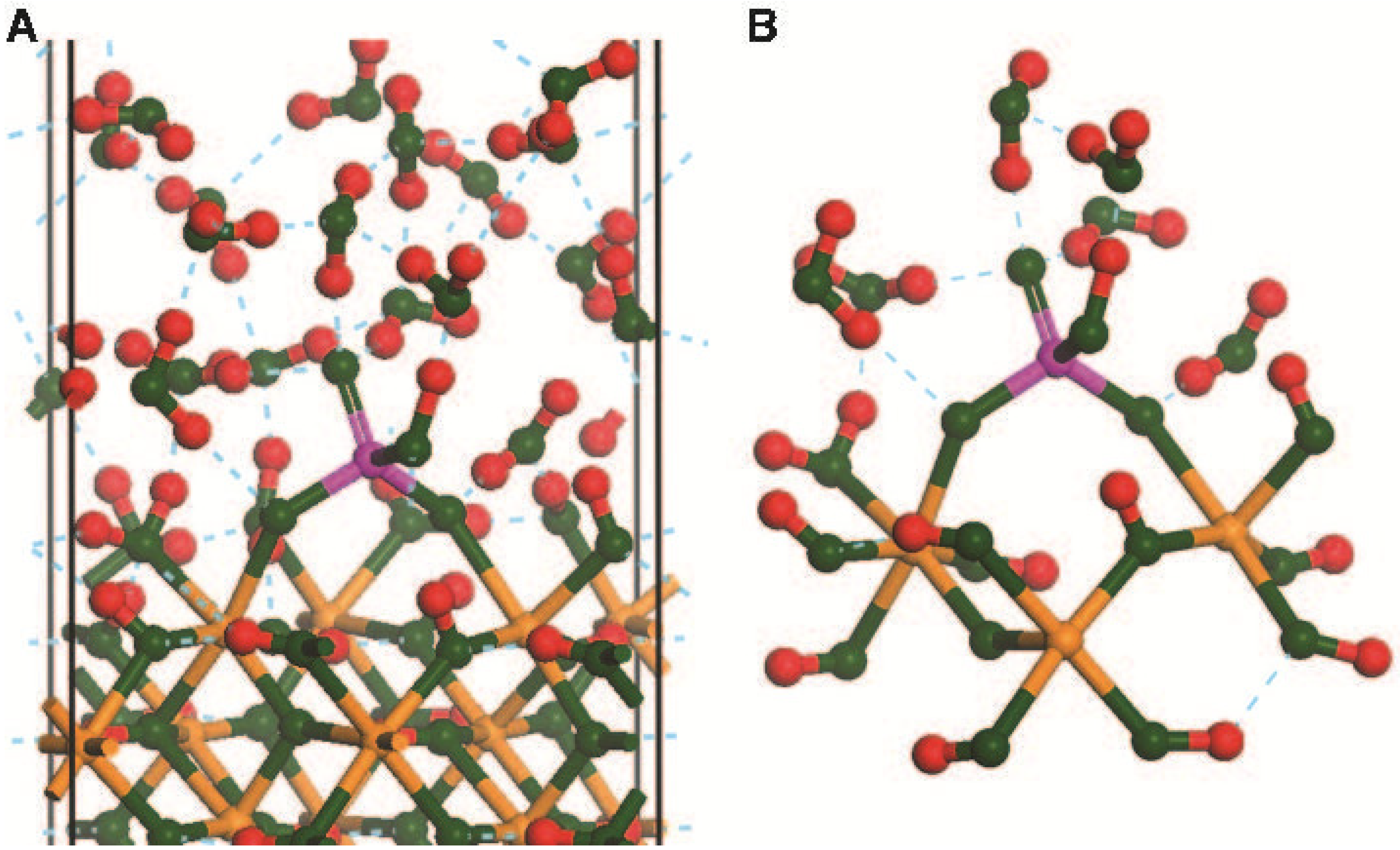
2.3. Planewave Calculations Using α-FeOOH (010)

The starting configuration for the periodic bidentate, binuclear HAsO42− on the goethite (α-FeOOH) (010) surface was taken from previous simulations of HPO42− on the same surface [135]. Phosphate and arsenate structures and chemistries are similar, so this starting configuration is a reasonable approximation. An energy minimization was performed on this starting configuration to allow the atoms to relax as necessary for the As for P substitution. Energy minimizations were carried out with the lattice parameters constrained the experimental values (9.24 × 9.95 Å2) [164] and with a vacuum gap between surface slabs of 10 Å. The model stoichiometry was 24FeOOH, HAsO42−, 29H2O, and 2H3O+ (Fe24O83H89As). The small model system size and the high percentage of H+ per H2O molecules severely limits the realism of the model compared to experimental systems, so the results from these calculations should be considered exploratory of model system behavior rather than an accurate portrayal of arsenate adsorption thermodynamics and kinetics.
Projector-augmented planewave calculations [152,165] with the Perdew-Erzenhof-Burke exchange correlation functional [160] were performed with the Vienna Ab-initio Simulation Package (VASP 5.2) [153,154,155,156,157]. The PBE0 exchange correlation functionals were Fe pv (14 valence e), O (6 valence e), H (1 valence e) and As (5 valence e) as labeled in the VASP exchange correlation functional library. Energy cut-offs (ENCUT in VASP input files) of 500 eV and 400 eV were used for energy minimizations and molecular dynamics simulations, respectively. The precision of the self-consistent field calculation of electron density was (PREC = Accurate = 700 eV/ROPT = −2.5 × 10⁻⁴) for energy minimizations and (PREC = Medium = 700 eV/ROPT = −2.5 × 10⁻³) for molecular dynamics simulations. The PREC-flag determines the energy cutoff (ENCUT) when no value is given for ENCUT in the central input file of VASP, INCAR, and the ROPT-tag controls the real-space optimization. The lower accuracies of the molecular dynamics (MD) simulations were chosen for practical reasons. Thousands of configurations and their energies need to be calculated for MD simulations, so the less stringent electron density grid speeds up the energy calculation at each step. The assumption here is that although the MD simulations are less accurate, they are not dramatically in error for predicting atomic structure. Thus, the MD simulations can be used to relax the atomic positions to achieve an approximate configuration and energy, and then energy minimizations can be performed to obtain structures and energies that are more precise. Without the MD simulations, the likelihood of the energy minimizations becoming trapped in a local potential energy minimum is much greater.
Periodic DFT calculations were run with 1 k-point created with the Monkhorst-Pack mesh. The DFT+U correction [166,167] was employed with a U = 4 eV for Fe and 0 eV for all other elements. Spin states were ordered according to the experimental observed magnetic ordering of goethite [168]. These selections have worked reasonably well in a previous study on goethite and goethite-water [73]. No dispersion-corrections were employed in these calculations although the results of DFT calculations of adsorption onto mineral surfaces may be affected by Van der Waals forces and how they are approximated [86]. The MD simulations were run at a temperature of 300 K maintained by the Nosé-Hoover thermostat [169]. Time steps were 0.5 fs (POTIM = 0.5). POTIM is a time-step variable and its value depends on the type of calculation being performed. Note that because some DFT methods may over structure and freeze water at 300 K, some authors have used higher temperatures to overcome this problem [170]. Another method is to use D instead of H [171], so that a 1 fs time step can be used instead of a 0.5 fs time step. Both are accepted practices, but we prefer to use the actual temperature and H atoms. This may cause error, but these errors are intrinsic to the method and as such not different in character from other computational uncertainties. Introducing errors by giving the atoms extra kinetic energy or mass may mask the discrepancies with experiment. Instead, highlighting these discrepancies is important and points to the need to improve computational methods.
Calculation of the periodic surface complex structures also allows for creation of more realistic molecular clusters that are surface specific. Figure 3 shows how an extended cluster (Figure 3B) can be extracted from the periodic model (Figure 3A). By selecting all the O atoms bonded to the Fe atoms connected to the As surface complex, a molecular cluster is created that retains surface-specific structure. The O atoms at the edge of the cluster are then terminated with H+ in order to satisfy valence and adjust the overall charge of the cluster as desired. Positions of hydration H2O molecules can be included in the extended cluster (Figure 3B) to better mimic the aqueous phase. The combination of periodic and molecular cluster DFT results can take advantage of the strengths of each approach. For example, the periodic calculations should provide more accurate surface structures and adsorption energies, but molecular cluster models can be used to predict IR, Raman, and NMR spectra [135].
Figure 3. (A) Periodic model of goethite and (B) an extended cluster extracted from the periodic model.
Minerals 04 00208 g003

3. Results and Discussion

The molecular cluster results show how the initial cluster charges affect Gibbs free energy of adsorption (ΔGads) of iAsV and iAsIII, the effect of hydration on ΔGads for the iAsV models, and compare the of adsorption energies of triprotic iAsIII, and monoprotic or diprotic iAsV onto hydrated neutral Fe clusters. The molecular cluster calculations also compare the calculated As—Fe distances with EXAFS data. In addition, calculations to determine the rate constant for iAsV adsorption on Fe clusters and periodic models are discussed.

3.1. Effect of Cluster Charge on ΔGads

Reactions (1)–(7) in Table 1 show the ΔGads of H3AsO3 (Reaction (1) and (2)), HAsO42− (Reaction (3) and (4)), and H2AsO4 (Reaction (5)–(7)) onto either a neutral (Fe2(OH)6(OH2)40) or +4 charged (Fe2(OH)2(OH2)84+). Reaction (7) is stoichiometrically equivalent to one previously reported; however, for our calculation we used an energy minimization convergence criteria of 0.03 kJ/mol, whereas Sherman and Randall [91] used 5 kJ/mol. Significantly, Sherman and Randall [91] reported that the reaction:
Fe2(OH)2(OH2)6H2AsO43+ (BB) + H2O → Fe2(OH)2(OH2)7H2AsO43+ (MM)
was endothermic and required +95 kJ/mol of energy; however, our results predict that this conversion would require +17 kJ/mol of Gibbs free energy. Both calculations predict that the BB structure is energetically favorable, but our results show energy difference between the BB and MM structures is not as large, and that these structures could co-exist in nature. The possibility of the presence of both BB and MM agree with prior research [130], but the lower ΔGads of the BB is inconsistent with the claim that MM adsorption is dominant [128]. The methodologies used to calculate the conversion of BB to MM could account for the calculated energy differences; the methods differ by:
  • Model convergence criteria;
  • Implicit solvation (our work) and gas-phase results from Sherman and Randall [91];
  • Electronic energies (ΔE) from Sherman and Randall [91] and ΔG for our work;
  • Use of a single, gas-phase minimized H2O model to balance Equation (2) [91], whereas we used 1/8 the energy of an implicitly solvated model with eight H2O molecules.
Throughout this work, unless otherwise noted, we used explicitly hydrated models for all of the reactants and products for the energy minimization calculations, and those same models for the implicitly solvated (i.e., IEFPCM) single-point energy calculations.
Table 1. Effect of Fe cluster charge on the ΔGads of iAsIII and iAsV.
Reaction #ReactionΔGads (kJ/mol)
(1)H3AsO3 + Fe2(OH)6(OH2)40 → Fe2(OH)4(OH2)4HAsO3 + 2H2O−60
(2)H3AsO3 + Fe2(OH)2(OH2)84+ + 16H2O → Fe2(OH)2(OH2)6HAsO32+ + 2H3O+·8H2O−159
(3)HAsO42− + Fe2(OH)6(OH2)40 + 8H2O → Fe2(OH)4(OH2)4HAsO4 + 2OH·4H2O+14
(4)HAsO42− + Fe2(OH)2(OH2)84+ → Fe2(OH)2(OH2)6HAsO42+ + 2H2O−263
(5)H2AsO4 + Fe2(OH)6(OH2)40 + 3H2O → Fe2(OH)4(OH2)4HAsO4 + OH·4H2O−309
(6)H2AsO4 + Fe2(OH)2(OH2)64+ + 7H2O → Fe2(OH)2(OH2)6HAsO42+ + H3O+·8H2O−336
(7)H2AsO4 + Fe2(OH)2(OH2)84+ → Fe2(OH)2(OH2)6H2AsO43+ + 2H2O−338
Comparing Reactions (1) with (2), (3) with (4), and (5) with (6) shows that the adsorption of iAs onto the more highly charged surfaces is more energetically favorable. However, it is unlikely that a +4 localized charged would occur in nature, and the results for ΔGads for the 0 charged Fe clusters are more realistic for exergonic adsorption of H3AsO3 and the endergonic adsorption of HAsO42−. The adsorption of H2AsO4 is energetically favorable, regardless of the initial Fe cluster charge (Reactions (5)–(7)).

3.2. Effect of Fe Cluster Hydration on ΔGads for Anhydrous and Octahydrated H2AsO4

Reactions (8)–(13) in Table 2 give examples of the effect of neutral Fe cluster hydration on the ΔGads of H2AsO4. The reactions differ only by the number of H2O molecules of hydration that are present on the initial Fe cluster (i.e., 0, 4, 8, or 8 for Reactions (8)–(11), respectively) and the HAsO42−-Fe cluster (i.e., 0, 4, 4, and 8, for Reactions (8)–(11), respectively). Reactions (12) and (13) used octahydrated H2AsO4 as the reactant. Note that we used a tetrahydrated hydroxide model to mass and charge balance Reactions (8)–(11).
Table 2. Effect of Fe cluster hydration (Reactions (8)–(11)) and iAsV hydration (Reactions (12) and (13)) on ΔGads of iAsV.
Reaction #ReactionΔGads (kJ/mol)
(8)H2AsO4 + Fe2(OH)6(OH2)4 + 3H2O → Fe2(OH)4(OH2)4HAsO4 + OH·4H2O−186
(9)H2AsO4 + Fe2(OH)6(OH2)4·4H2O + 3H2O → Fe2(OH)4(OH2)4HAsO4·4H2O + OH·4H2O−195
(10)H2AsO4 + Fe2(OH)6(OH2)4·8H2O → Fe2(OH)4(OH2)4HAsO4·4H2O + OH·4H2O + H2O−217
(11)H2AsO4 + Fe2(OH)6(OH2)4·8H2O + 3H2O → Fe2(OH)4(OH2)4HAsO4·8H2O + OH·4H2O−223
(12)H2AsO4·8H2O + Fe2(OH)6(OH2)4·4H2O → Fe2(OH)4(OH2)4HAsO4·4H2O + OH·4H2O + 5H2O−64
(13)H2AsO4·8H2O + Fe2(OH)6(OH2)4·8H2O → Fe2(OH)4(OH2)4HAsO4·4H2O + OH·4H2O + 5H2O−86
As the H2O molecules of hydration increases from Fe2(OH)6(OH2)4 to Fe2(OH)6(OH2)4·8H2O (Reactions (8)–(11)), the ΔGads of H2AsO4 becomes more negative. Reactions (10) and (11) differ only by the numbers of H2O molecules present on the cluster product, the HAsO42−-Fe cluster, four for Reaction (10) and eight for Reaction (11). The ΔGads for Reactions (10) and (11) differ by 6 kJ/mol, which is less than the ±10 kJ/mol error associated with thermodynamics calculations, so the results are indistinguishable. Using eight hydrating H2O molecules on the HAsO42−-Fe cluster rather than four significantly increased the time need to minimize the model. Significantly, Reactions (12) and (13), where iAsV is present as octahydrated H2AsO4 exhibit ΔGads that are likely more realistic than those seen for ΔGads of anhydrous H2AsO4 (Reactions (8)–(11)). Reactions (8)–(11) are shown here to emphasize the cluster hydration results. Therefore, we used the anhydrous H2AsO4 reactant in Reactions (8)–(11) because these calculations are focusing on the hydration state of the clusters and are used here as a teaching tool. To attain results that are meaningful with respect to nature and experimental conditions, all of the products and reactants should be hydrated.
Recently [122], a claim was made that using a single explicit H2O molecule and implicit solvation with the self-consistent reaction field (SCRF) COSMO [133,134] could produce superior results to using multiple H2O molecules. This argument is based on calculations that used small, monohydrated organic and inorganic molecules in the COSMO SCRF that showed better agreement with experiment when a single, rather than multiple H2O molecules were used to hydrate the models [172]. However, the work that modeled iAsV interacting with ferric hydroxide clusters assumed that the result from simple organic and inorganic molecules would be applicable for the cluster calculations [122]; they did not test models with more than one H2O molecule.
One argument for the addition of multiple H2O molecules is that the model would better approximate the aqueous environment in which As adsorption occurs. However, if the multiple H2O molecules are arranged in a way that does not lead to an observable PES minimum (i.e., becoming trapped in a local minimum), then using more than one H2O molecule could lead to errors. On the other hand, the results for Reactions (12) and (13) suggest that multiple H2O of hydration for all products and reactants could lead to results that are chemically more realistic than reactions with anhydrous reactants and products. Furthermore, chemical properties such as vibrational frequencies [75] are dependent on hydrogen bonding, so the inclusion of additional explicit H2O molecules could be necessary to calculate precise spectroscopic and structural results.
Our work used the IEFPCM, and not the COSMO reaction field used by Farrell and Chaudhary [122]. A particular quantum chemistry method such as the SCRF, DFT method, or basis set can be useful for precisely calculating particular chemical properties, such as energies, but may produce other chemical properties that are imprecise. In this instance, the COSMO SCRF was parameterized to work most successfully with limited explicit hydration, but other SCRF such as IEFPCM may require the addition of more H2O molecules to obtain precise results. Furthermore, particular DFT methods have been developed that are useful for calculating energies, geometries, and kinetics [138,173,174], whereas other DFT methods are useful for calculating spectroscopic properties such as NMR chemical shifts for H and C [175,176]. Because the exact Exc for DFT is unknown, it is not yet possible to use one DFT method to calculate every chemical property. Therefore, it is necessary when doing DFT calculations to read the literature to find methodologies that are efficient for calculating the chemical properties of interest and to be willing to experiment with variations of those methods, if the calculated results are imprecise when compared with experimental data. This procedure is similar to those an experimentalist takes when deciding how to study a chemistry of interest.

3.3. Effect of As Oxidation State and DFT Method on ΔGads

Reactions (14)–(19) in Table 3 show the ΔGads of octahydrated H3AsO3, HAsO42−, and H2AsO4 onto tetra- and octahydrated Fe2(OH)6(OH2)40. The ΔGads for iAsIII is more favorable than it is for iAsV; this is fortunate, if correct, because iAsIII is more toxic than iAsV is. The results for the preferential adsorption of iAsIII over iAsV at the point-of-zero charge for the Fe cluster are supported by experimental data that shows the same trend [101]. Under acidic or basic conditions, the Fe clusters would have charges, and neutral H3AsO3 might not adsorb to Fe surfaces as favorably. Conversely, although these reactions show less favorable adsorption of octahydrated HAsO42− and H2AsO42− to the neutral Fe cluster than for iAsIII, under acidic or basic conditions when the cluster is charged, the charged iAsV ions could adsorb more favorably than uncharged iAsIII. Although the products and reactants are anhydrous, Reactions (1)–(7) support this assertion, where neutral H3AsO3 adsorbs more strongly to the neutral cluster (Reaction (1)) than to the +4-charged cluster (Reaction (2)). Conversely, the charged iAsV reactants in Reactions (3)–(7) adsorb more strongly to the +4-charged clusters than they do to the neutral clusters. These results that show weaker adsorption of H3AsO3 and stronger adsorption of charged iAsV to charged Fe clusters are also supported by experimental data [101]. Furthermore, the results for Reactions (14) and (15) show that HAsO42− would adsorb less favorable to the neutral Fe cluster than does H2AsO4. Note that a tetrahydrated hydroxide model was used to mass and charge balance Reactions (14)–(17); the hydroxide was not necessary to mass charge balance Reactions (12) and (13).
Table 3. Effect of As oxidation state on BB adsorption to neutral Fe clusters. For Reaction (16), the density functional theory (DFT) methods used to calculate ΔGads were: a, B3LYP; b, PBE0; and c, M06-L.
Reaction #ReactionΔGads (kJ/mol)
(12)H3AsO3·8H2O + Fe2(OH)6(OH2)4·4H2O → Fe2(OH)4(OH2)4HAsO3·4H2O + 10H2O−124
(13)H3AsO3·8H2O + Fe2(OH)6(OH2)4·8H2O → Fe2(OH)4(OH2)4HAsO3·4H2O + 10H2O−146
(14)HAsO42−·8H2O + Fe2(OH)6(OH2)4·4H2O → Fe2(OH)4(OH2)4HAsO4·4H2O + 2OH·4H2O+15
(15)HAsO42−·8H2O + Fe2(OH)6(OH2)4·8H2O → Fe2(OH)4(OH2)4HAsO4·4H2O + 2OH·4H2O + 4H2O−6
(16)H2AsO4·8H2O + Fe2(OH)6(OH2)4·4H2O → Fe2(OH)4(OH2)4HAsO4·4H2O + OH·4H2O + 5H2O−64 a, −35 b, −3 c
(17)H2AsO4·8H2O + Fe2(OH)6(OH2)4·8H2O → Fe2(OH)4(OH2)4HAsO4·4H2O + OH·4H2O + 5H2O−86
For Reaction (16), we compared the ΔGads calculated with the B3LYP, PBE0, or M06-L DFT methods. The ΔGads calculated with B3LYP (−64 kJ/mol), M06-L (−3 kJ/mol), and PBE0 (−35 kJ/mol) results all predict favorable, exergonic reactions. These results show that calculated thermodynamic results are dependent on the chosen DFT method. Because the adsorption of iAsV is experimentally observed over a wide pH range [101], the results from B3LYP, PBE0, or M06-L could be correct. Thermodynamic results from DFT calculations are typically precise within ±10 kJ/mol; therefore, the B3LYP results would range from −74 to −54 kJ/mol and the PBE0 results would range from −45 to −25 kJ/mol; these results do not overlap, so the precision of the results from B3LYP and PBE0 differ. Within the ±10 kJ/mol error range of DFT methods, the M06-L results would range from −13 to +7 kJ/mol; therefore, because iAsV adsorption is favorable, the M06-L results could be erroneous.

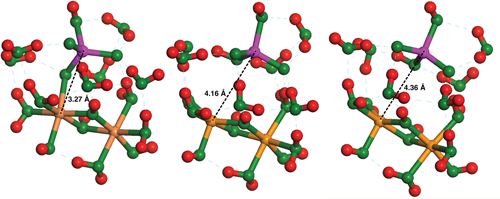
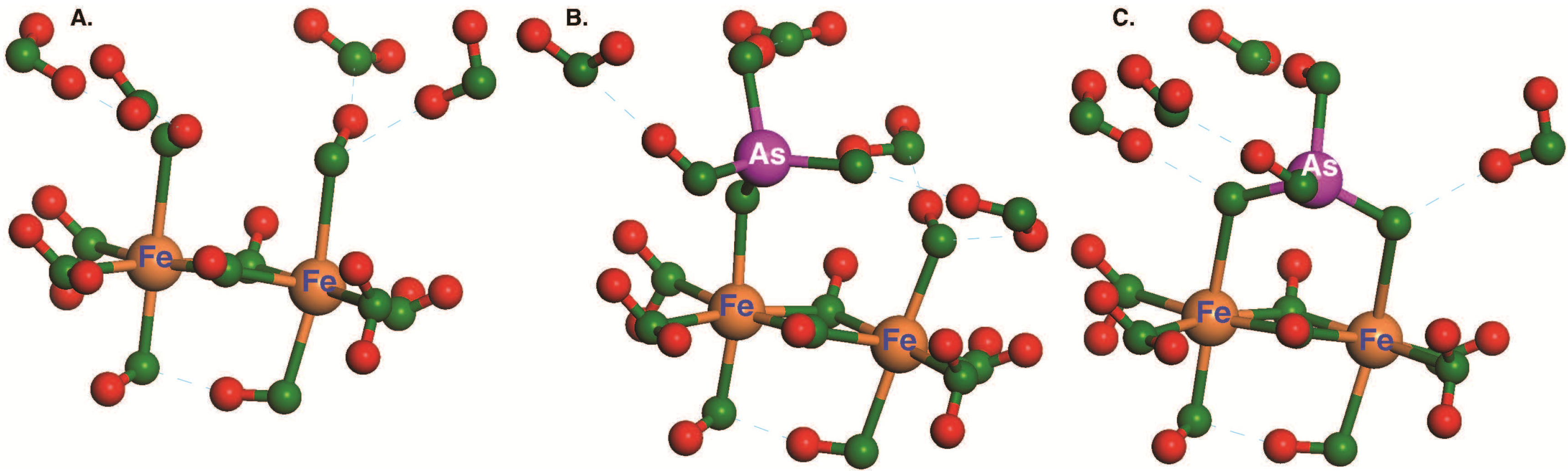
3.4. As—Fe Distance and As-O Bond Length Data from Experiments Compared with Cluster and Periodic Model Results

Table 4 shows the BB As—Fe distances and As-O bond distances calculated from this work for AsIII and AsV, the calculated BB results of Sherman and Randall [91] for AsV, and EXAFS data for AsIII and AsV on four mineral surfaces.
Notably, that the Fe2(OH)2(OH2)6H2AsVO43+ (BB) model [91] exhibits four As-O bonds, two of which are As-OH bonds that are 1.73 Å. Sherman and Randall [91] observed a 1.62–1.64 Å As-O bond with EXAFS that is not present in their models where H2AsO4 has two As-OH single bonds to the As atom. We argue that the 1.62–1.64 Å As-O bond is an As-O double bond (As=O) that our calculations predict to be 1.63 Å due to HAsO42− being adsorbed to the Fe surface (model Fe2(OH)4(OH2)4HAsVO4 (BB)), rather than a As-OH single bond, and that iAsV is not present on Fe surfaces as H2AsO4 with two As-OH single bonds. However, we also note that the Fe2(OH)4(OH2)4HAsVO4 (BB) model is not hydrated with explicit H2O molecules and that when the model is hydrated with either four or eight explicit H2O molecules, the As=O bond length increases from 1.63 to 1.67 Å, which is slightly longer than the observed 1.62–1.64 Å As=O length, but is still shorter than the 1.73 Å bond lengths from the model of Sherman and Randall [91]. In Table 4, we report the results for the +3-charged model that was energy minimized using the methods described in this work. The As-OFe and As-OH bond distances calculated here differ by 0.01 Å from those reported by Sherman and Randall [91], whereas the As—Fe distances calculated here are both 0.05 Å shorter than those reported by Sherman and Randall [91]. The difference in As—Fe distances likely occur due to differences in methodology, but the results from both models lie within the range of experimental uncertainty.
Table 4. As—Fe interatomic distance, As-OFe bond distance, and As-O bond distance results from this work compared to previous calculations and extended X-ray adsorption fine structure (EXAFS) data for AsV and AsIII adsorption onto ferrihydrite (Fh), hematite (Hm), goethite (Gt), and lepidocrocite (Lp). For Fe2(OH)4(OH2)4HAsVO4·4H2O (BB), the DFT methods used to calculate ΔGads were: x, B3LYP; y, PBE0; and z, M06-L.
AsV ComplexAs—Fe (Å)As—Fe (Å)As-OFe (Å)As-OFe (Å)As-OH (Å)As-OH (Å)As=O (Å)
Fe2(OH)4(OH2)4HAsVO4 (BB)3.133.251.711.731.83 1.63
Fe2(OH)4(OH2)4HAsVO4·4H2O (BB)3.20 x, 3.19 y, 3.08 z3.28 x, 3.24 y, 3.29 z1.69 x, 1.68 y, 1.69 z1.72 x, 1.71 y, 1.72 z1.76 x, 1.75 y, 1.79 z 1.67 x, 1.66 y, 1.65 z
Fe2(OH)4(OH2)4HAsVO4·8H2O (BB)3.303.301.701.701.76 1.67
Goethite (010) periodic model (BB)3.563.681.721.721.78 1.73
Fe2(OH)2(OH2)6H2AsVO43+ (BB)3.243.241.701.701.721.72
Fe2(OH)2(OH2)6H2AsVO43+ (BB) a3.293.291.711.711.731.73
AsV on Fh (BB) a3.273.381.701.701.67 1.64
AsV on Gt (BB) a3.303.301.701.701.70 1.63
AsV on Lp (BB) a3.303.321.711.711.66 1.63
AsV on Hm (BB) a3.243.351.701.701.70 1.62
AsV on Fh (BB) b3.25 (±0.02)
AsV on Gt (BB) b3.28 (±0.01)
AsV on Lp (BB) c3.31 (±0.014) 1.69 (±0.004)
AsV on Gt (BB) c3.30 (±0.008) 1.69 (±0.004)
AsV on Fh (BB) d3.27
Goethite (010) periodic model (MM)3.545.00 †1.781.751.71 ‡ 1.68
AsV on Gt e3.25 § 1.689 1.679
AsIII ComplexAs—Fe (Å)As—Fe (Å)As-O (Å)As-O (Å)As-O (Å)As=O (Å)
Fe2(OH)4(OH2)4HAsIIIO3·4H2O (BB)3.263.411.771.74 1.90na
Fe2(OH)4(OH2)4HAsIIIO3·8H2O (BB)3.293.391.781.72 1.90
AsIII on Lp (BB) c3.41 (±0.013) 1.78 (±0.014)
AsIII on Gt (BB) c3.31 (±0.013) 1.78 (±0.012)
AsIII on Fh (BB) d3.41–3.44
AsIII on Fh and Hm (BB) f3.35 (±0.05)
AsIII on Gt and Lp (BB) f3.3–3.4
AsIII on Gt (BB) g3.378 (±0.014)
Notes: a Sherman and Randall [91]; b Waychunas et al. [89]; c Farquhar et al. [82]; d Gao et al. [87]; e Loring et al. [128]; f Ona-Nguema et al. [92]; g Manning et al. [81]. This As—Fe distance does not agree with that reported by Loring et al. [128] for a MM. For the MM periodic model, there is one As-OH bond and two As partial double bonds (1.71 and 1.68 Å), because HAsO42− is adsorbed to the surface. § For the Loring et al. [128] model, both As-O bonds are aprotic and should have partial double bonds.
For the iAsV models, the two calculated As—Fe distances within each configuration differ by 0.12, 0.08, and 0.00 Å from each other for the Fe2(OH)4(OH2)4HAsVO4, Fe2(OH)4(OH2)4HAsVO4·4H2O, and Fe2(OH)4(OH2)4HAsVO4·8H2O models, respectively. Sherman and Randall [91] reported two As—Fe distances for ferrihydrite (Fh), lepidocrocite (Lp), hematite (Hm), and goethite (Gt), whereas the other data report a single As—Fe distance for the adsorption onto Fh, Gt, or Lp. The AsV—Fe distance results from the Fe2(OH)4(OH2)4HAsVO4·8H2O model agree within experimental uncertainty with the Gt and Lp data of Sherman and Randall [91], the Gt and Fh data of Waychunas et al. [89], and the Gt and Lp data of Farquhar et al. [82]. The data for the AsV—Fe distances overlap for the minerals used for these studies; therefore, determining the type of mineral to which the iAsV is bonding could be difficult; however, we can state that the Fe cluster models are predicting As—Fe distances that are indicative of BB adsorption of AsV. Similarly, the calculated experimental and AsV—OFe bond distances agree precisely.
For the BB results for the periodic structures of α-FeOOH (010), the As-OFe bonds (1.72 Å) show precise agreement with experiment and correlate well with the cluster results. However, the As—Fe distances (3.56 and 3.68 Å) both overestimate the experimental data, and the As-OH and As=O bonds both overestimate the experimentally observed bond distances. For the MM periodic model, the calculated As—Fe distance is overestimating the 3.25 Å distance measured distance of Loring et al. [128] by 0.29 Å. The errors associated with the periodic calculations could be due to systematic errors in the planewave calculations or could be because the α-FeOOH (010) surface is not the surface where As adsorption predominately occurs.
The two AsIII—Fe bond distances in the Fe2(OH)4(OH2)4HAsIIIO3·4H2O model differ by 0.15 Å and by 0.10 for the octahydrated version of that model., The longer calculated As—Fe distances (ca. 3.4 Å) agree with most of the AsIII data within uncertainty, whereas the shorter calculated As—Fe distance agrees well with the data of Gao et al. [87]. Again, because of the data overlap and due to the uncertainty in the As—Fe distances observed for AsIII adsorption onto Hm, Gt, Lp, and Fh, it is difficult to resolve different sorption mechanisms of various Fe-oxide and Fe-hydroxide minerals; however, it is possible to state the BB adsorption is occurring. Furthermore, it is possible to differentiate AsIII—Fe and AsV—Fe BB adsorption, because the former distances are approximately 3.4 Å, whereas the latter are approximately 3.3 Å. Significantly, these distances are seen both experimentally and computationally. Moreover, there is good agreement between the calculated AsIII-OFe distance and the EXAFS data of Sherman and Randall [91].
For the Fe2(OH)4(OH2)4HAsVO4·4H2O (BB) model, we compared the As—Fe distance results obtained from the B3LYP, PBE0, and M06-L methods. For the As—Fe distances, the B3LYP (3.20 Å) and PBE0 (3.19 Å) results correlate for one of the As—Fe distance, and the B3LYP (3.28 Å) and M06-L (3.29 Å) results agree for the other As—Fe distance. The As-O and As=O bond lengths agree well among the DFT methods and agree precisely with the experimental data in Table 4. This type of DFT method testing helps eliminate the possible effects of exchange-correlation functional errors on the results.
The Fe2(OH)4(OH2)4HAsVO4·4H2O (BB) model used for these DFT method comparisons is the adsorption product of Reaction (16), and the M06-L ΔGads results for Reaction (16) ranged from −13 to +7 kJ/mol, suggesting thermodynamic adsorption results from M06-L that are potentially unfavorable, relative to the results from B3LYP and PBE0 (Table 3). In addition, the 3.08 Å As—Fe distance from the M06-L minimized model (Table 4) is predicts is significantly shorter than the experimental data and the results from B3LYP and PBE0. Therefore, because the As—Fe distance calculated with M06-L is imprecise, it is likely that the ΔGads results from M06-L is also imprecise.
Notably, the PBE0 As—Fe distance results from the cluster and periodic calculations differed distinctly. The cluster results underestimated the As—Fe distance data by approximately 0.1 Å, whereas the periodic calculation results overestimated those data by approximately 0.25 Å. The PBE0 method, like many DFT methods, may contain different parameters, depending on which software package implements it (e.g., VASP, Gaussian 09, etc.), so the results obtain with a particular DFT method using different software packages might not be directly comparable. In addition to the potential differences in the DFT methods, model sizes could also contribute to the discrepancies in the calculated distances obtained from the periodic and cluster models. One would presume that the larger periodic models would provide results that are more precise relative to the data than the smaller cluster models do; however, neither model size produced precise As—Fe distances. Differences between periodic and cluster model results have been discussed previously [73,135].

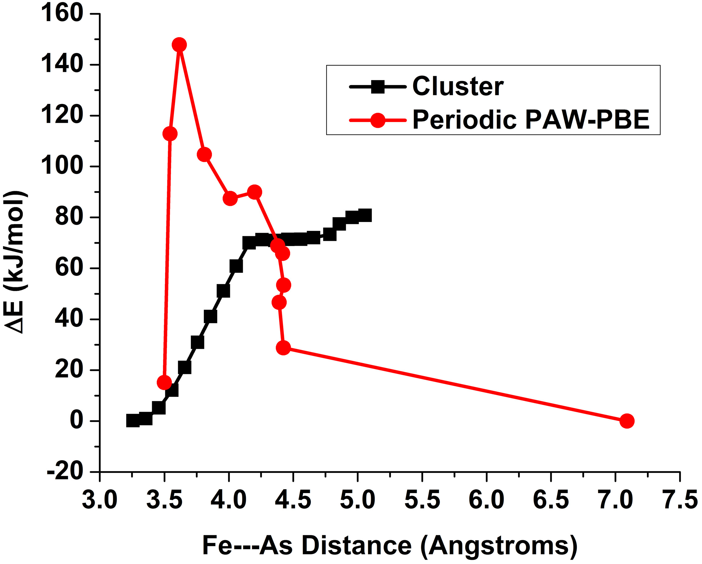
3.5. Sorption Kinetics for iAsV on Cluster and Periodic Models

Calculations were completed to show a possible reaction pathways for desorption of the monodentate inner-sphere complex of HAsO42− from Fe3+-(oxyhydr)oxide cluster and from the periodic goethite (010) surface. Although the bidentate binuclear complex is likely to be more stable [88,91], the monodentate species is an intermediate between the bidentate and outer-sphere species. Figure 4 shows desorption of iAsV from a Fe2(OH)4(H2O)5-HAsO4 cluster model, where the model begins as a MM structure with a As—Fe distance of 3.27 Å (Figure 4A), moves through a transition state structure (Figure 4B), and reaches the outer-sphere structure (Figure 4C) where the As—Fe distance is 4.36 Å. The Fe—As distances were increased manually and then held constant in each calculation until there ceased to be a bonding interaction. The energies of the monodentate reaction pathway are portrayed as a function of the Fe—As distance in the Figure 4 for both periodic and cluster models.
Figure 4. Desorption of iAsV from Fe clusters showing (A) the initial MM model, (B) the transition state model, and (C) the outer-sphere, final structure model.
Minerals 04 00208 g004
Based on the results shown in Figure 5, ΔEa for the breaking of the first bond in monodentate complex requires approximately +133 and +70 kJ/mol in the periodic and cluster models, respectively. (Note that there is a small increase in energy of the model system near a Fe—As distance of 4.2 Å, but this energy increase is insignificant compared to the first barrier.) The energy barrier for the reverse reaction is higher, +148 kJ/mol, in the periodic model because the outer-sphere complex is lower in energy in this model. The higher energy of the inner-sphere complex and the high-energy barrier of adsorption suggest that adsorption would not occur to the goethite (010) surface under these conditions; this result corroborates with the discussion the long As—Fe distances reported in the previous section for the periodic models. In the molecular cluster models, the adsorption reaction barrier is insignificant, i.e., +1 kJ/mol. We strongly remind the reader, however, that the conditions of this model are not realistic compared to experimental conditions where lower H+ activity, lower arsenate concentrations and greater volume of water would exist and affect the results. On the other hand, the cluster models exhibit almost no energy barrier to adsorption from outer-sphere to monodentate with the inner-sphere complex having a lower energy (Figure 5).
Figure 5. Constrained scan of Fe—As distances starting from monodentate configuration to outer-sphere using periodic and molecular cluster DFT calculations results in ΔEa of adsorption of +148 and +1 kJ/mol, respectively and desorption of +133 and +70 kJ/mol, respectively.
Minerals 04 00208 g005
The discrepancies between the two types of models are illustrative of some of the problems that can be encountered by each type of approach. First, although the periodic models were run for short (i.e., 6000 steps × 0.5 fs = 3 ps) molecular dynamics simulations at 300 K to relax the atoms, the complex nature of the periodic model all but ensures that a global minimum configuration will not be obtained. This is an example of a general problem, i.e., adding more atoms to the simulation may make it more realistic but increases the number of potential energy minima dramatically. Thus, the transition state may overestimate the ΔEa because the system is not in the lowest possible potential energy configuration, especially with respect to the configuration of H2O molecules.
There are numerous possibilities for overcoming the metastable minimum problem. Longer simulation runtimes are one option. These longer simulations could be performed with tight-binding DFT (i.e., DFT-B; see REF for a review of DFT-B) or classical force fields. However, one problem with classical simulations is that it is difficult to created accurate parameterizations that allow for bond-making and bond-breaking, especially for configurations far from equilibrium such as transition states (see [71] for a review). Replicate MD simulations are another option for exploring configuration space. These require multiple simulations at different temperatures to be run simultaneously such that higher and lower temperature configurations can be switched with potential energies overlap. Again, however, this method requires a significant expansion of computational effort to run the multiple MD simulations.
Alternatively, the cluster model allows the “surface” atoms to relax without constraint from the remainder of the crystal, which may help explain the lower ΔEa. The “outer-sphere” configuration is higher in energy in this case because the HAsO42− is not completely solvated by the six extra H2O molecules in the model. In addition to the loss of solvation energy, protonation of the HAsO42− does not occur in the cluster whereas in the periodic model H2AsO4 is the product.
Even with these discrepancies in the energies and products between the periodic and cluster models, the structures of the reactants and transition states are similar. A combined approach using insights from both periodic and cluster models is useful at this time because each has strengths and weaknesses. These first simulations of the reaction path can be reiterated by performing longer MD simulations at various steps and by searching for lower energy points along the reaction path. In addition, lower energy transition states determined via the cluster approach can be used to guide construction of transition states in the more realistic (but more complex) periodic simulations.
The main problem in this case, however, is likely to be that the (010) surface is not the dominant face responsible for adsorbing arsenate onto goethite. Thus, extensive calculations of any type could prove futile in terms of reproducing the observed ΔEa of adsorption/desorption. Other surfaces could be examined, because the (010) surface may not be the most preferred surface for adsorption of arsenate onto goethite. We had selected the (010) surface for arsenate adsorption onto goethite based on the analogy with chromate adsorption [177,178]. Recent DFT calculations have been used to suggest that the (210) surface adsorbs phosphate more strongly than the (010) surface [135]. None of the three just-mentioned studies included arsenate, however, so we are using the other oxyanions as analogs for arsenate. Our future computational work will focus on arsenic sorption reaction mechanisms onto the (210) surface, and this work would benefit from experiments similar to those that used chromate [177]. This point emphasizes that realistic model construction is one of the most important considerations in performing computational geochemistry. Too often, missing components are some inaccuracy in the original model creation leads to discrepancies with observation that cannot be resolved with even the most accurate quantum mechanical calculations.

4. Conclusions

This work explored the effect of cluster charge, hydration, As oxidation state, and DFT methods on the Gibbs free energy of adsorption (ΔGads) of inorganic arsenic (iAs) species onto Fe3+-(oxyhydr)oxide models. In general neutral clusters and hydrated models produced ΔGads results that are likely more realistic than models with charged clusters and anhydrous models. As shown with experiments [101], iAsIII adsorption onto neutral Fe3+-(oxyhydr)oxide cluster models was more exergonic than iAsV adsorption onto the same cluster models. For the DFT calculations on the clusters, the results showed that both ΔGads and As—Fe distances depend on the DFT method used to calculate those properties; however the As—Fe distance results from these calculations generally agreed precisely with the experimental data cited.
The cluster model As—Fe distance and As-O bond distance results showed relatively precise agreement with the experimental data. Conversely, the periodic planewave calculation results for iAsV adsorption onto α-FeOOH (010) generally overestimated the As—Fe distance and As-O bond length data for iAsV adsorption onto goethite. Other α-FeOOH surfaces could produce results that are more precise.
Sorption kinetics calculations using DFT with cluster and a periodic model of α-goethite (010) showed discrepancies in the calculated activation energies of iAsV adsorption. One major difference for the discrepant results could be that the relatively large periodic model did not reach an energy minimum during the DFT MD simulation, whereas the cluster model was smaller than the periodic model and did attain a PES minimum. Although the calculated activation energies for the two methods differed, the initial and transition state structures for both calculations were structurally similar. Longer DFT MD simulations and periodic structures other than the (010) surface of α-FeOOH could produce results that are more precise.
The calculated reaction rates, thermodynamics, and structural results presented in this work provide results that could lead to a better understanding of the adsorption of arsenic to Fe (oxyhydr)oxide minerals. However, further studies are necessary to better determine which DFT methods produce the most precise results, the effect of model size on model precision, and the effects of model hydration and surface charge on As adsorption to Fe (oxyhydr)oxide models. Furthermore, basis set size, which was not addressed herein, could potentially affect the precision of the results for the cluster models; therefore, future studies should include the evaluation of basis set effects. Furthermore, increased collaborative efforts among experimental and computational (geo)chemists could lead to improved knowledge about arsenic adsorption on Fe minerals.

Acknowledgments

The authors would like to thank Hind A. Al-Abadleh, Associate Director at the Laurier Centre for Women in Science (WinS) for her help with editing and improving this paper. We also thank Benjamin Tutolo for running preliminary calculations on arsenate desorption who was supported by a research experience for undergraduates grant from the National Science Foundation under Grant No. CHE-0431328 (the Center for Environmental Kinetics Analysis, an NSF-DOE environmental molecular sciences institute). Computational support was provided by the Research Computing and Cyberinfrastructure group at The Pennsylvania State University. Lorena Tribe acknowledges support of the Research Collaboration Fellowship funded by The Pennsylvania State University.

Author Contributions

Heath D. Watts did the work reported in Section 3.1, Section 3.2, Section 3.3 and Section 3.4. James D. Kubicki and Lorena Tribe did the work reported in Section 3.5. All authors contributed to the preparation and writing of the manuscript.

Conflicts of Interest

The authors declare no conflict of interest.

References and Notes

  1. Kim, K.-W.; Chanpiwat, P.; Hanh, H.T.; Phan, K.; Sthiannopkao, S. Arsenic geochemistry of groundwater in Southeast Asia. Front. Med. 2011, 5, 420–433. [Google Scholar]
  2. Smedley, P.L.; Kinniburgh, D.G. A review of the source, behaviour and distribution of arsenic in natural waters. Appl. Geochem. 2002, 17, 517–568. [Google Scholar] [CrossRef]
  3. Anawar, H.M.; Akai, J.; Mihaljevič, M.; Sikder, A.M.; Ahmed, G.; Tareq, S.M.; Rahman, M.M. Arsenic contamination in groundwater of bangladesh: Perspectives on geochemical, microbial and anthropogenic issues. Water 2011, 3, 1050–1076. [Google Scholar] [CrossRef]
  4. Drewniak, L.; Maryan, N.; Lewandowski, W.; Kaczanowski, S.; Sklodowska, A. The contribution of microbial mats to the arsenic geochemistry of an ancient gold mine. Environ. Pollut. 2012, 162, 190–201. [Google Scholar] [CrossRef]
  5. Signes-Pastor, A.; Burló, F.; Mitra, K.; Carbonell-Barrachina, A.A. Arsenic biogeochemistry as affected by phosphorus fertilizer addition, redox potential and pH in a west Bengal (India) soil. Geoderma 2007, 137, 504–510. [Google Scholar] [CrossRef]
  6. Oremland, R.S.; Stolz, J.F. The ecology of arsenic. Science 2003, 300, 939–944. [Google Scholar] [CrossRef]
  7. Dhuldhaj, U.P.; Yadav, I.C.; Singh, S.; Sharma, N.K. Microbial interactions in the arsenic cycle: Adoptive strategies and applications in environmental management. Rev. Environ. Contam. Toxicol. 2013, 224, 1–38. [Google Scholar]
  8. Moreno-Jiménez, E.; Esteban, E.; Peñalosa, J.M. The fate of arsenic in soil-plant systems. Rev. Environ. Contam. Toxicol. 2012, 215, 1–37. [Google Scholar]
  9. Wolfe-Simon, F.; Blum, J.S.; Kulp, T.R.; Gordon, G.W.; Hoeft, S.E.; Pett-Ridge, J.; Stolz, J.F.; Webb, S.M.; Weber, P.K.; Davies, P.C.W.; et al. A bacterium that can grow by using arsenic instead of phosphorus. Science 2011, 332, 1163–1166. [Google Scholar] [CrossRef]
  10. Wolfe-Simon, F.; Blum, J.S.; Kulp, T.R.; Gordon, G.W.; Hoeft, S.E.; Pett-Ridge, J.; Stolz, J.F.; Webb, S.M.; Weber, P.K.; Davies, P.C.W.; et al. Response to comments on “A bacterium that can grow using arsenic instead of phosphorus.”. Science 2011, 332, 1149–1149. [Google Scholar]
  11. Masscheleyn, P.H.; Delaune, R.D.; Patrick, W.H. Arsenic and selenium chemistry as affected by sediment redox potential and pH. J. Environ. Qual. 1991, 20, 522–527. [Google Scholar] [CrossRef]
  12. Cullen, W.R.; Reimer, K.J. Arsenic speciation in the environment. Chem. Rev. 1989, 89, 713–764. [Google Scholar] [CrossRef]
  13. Greenwood, N.N.; Earnshaw, A. Arsenic, Antimony and Bismuth. In Chemistry of the Elements; Pergamon Press: Oxford, UK, 1997; pp. 547–599. [Google Scholar]
  14. Masscheleyn, P.H.; Delaune, R.D.; Patrick, W.H. Effect of redox potential and pH on arsenic speciation and solubility in a contaminated soil. Environ. Sci. Technol. 1991, 25, 1414–1419. [Google Scholar] [CrossRef]
  15. Flis, I.E.; Mishchenko, K.P.; Tumanova, T.A.; Russ, J. Dissociation of arsenic acid. J. Inorg. Chem. 1959, 4, 120–124. [Google Scholar]
  16. Francesconi, K.A. Arsenic species in seafood: Origin and human health implications. Pure Appl. Chem. 2010, 82, 373–381. [Google Scholar] [CrossRef]
  17. Beauchemin, S.; Fiset, J.-F.; Poirier, G.; Ablett, J. Arsenic in an alkaline AMD treatment sludge: Characterization and stability under prolonged anoxic conditions. Appl. Geochem. 2010, 25, 1487–1499. [Google Scholar] [CrossRef]
  18. Cheng, H.; Hu, Y.; Luo, J.; Xu, B.; Zhao, J. Geochemical processes controlling fate and transport of arsenic in acid mine drainage (AMD) and natural systems. J. Hazard. Mater. 2009, 165, 13–26. [Google Scholar] [CrossRef]
  19. Cramer, S.P.; Siskin, M.; Brown, L.D.; George, G.N. Characterization of arsenic in oil shale and oil shale derivatives by X-ray absorption spectroscopy. Energy Fuels 1988, 2, 175–180. [Google Scholar] [CrossRef]
  20. Pelley, J. Commonarsenical pesticide under scrutiny. Environ. Sci. Technol. 2005, 39, 122–123. [Google Scholar] [CrossRef]
  21. Arai, Y.; Lanzirotti, A.; Sutton, S.; Davis, J.A.; Sparks, D.L. Arsenic speciation and reactivity in poultry litter. Environ. Sci. Technol. 2003, 37, 4083–4090. [Google Scholar]
  22. Argos, M.; Kalra, T.; Rathouz, P.J.; Chen, Y.; Pierce, B.; Parvez, F.; Islam, T.; Ahmed, A.; Rakibuz-Zaman, M.; Hasan, R.; et al. Arsenic exposure from drinking water, and all-cause and chronic-disease mortalities in Bangladesh (HEALS): A prospective cohort study. Lancet 2010, 376, 252–258. [Google Scholar]
  23. Chen, Y.; Graziano, J.H.; Parvez, F.; Liu, M.; Slavkovich, V.; Kalra, T.; Argos, M.; Islam, T.; Ahmed, A.; Rakibuz-Zaman, M.; et al. Arsenic exposure from drinking water and mortality from cardiovascular disease in Bangladesh: Prospective cohort study. Br. Med. J. 2011, 342, d2431. [Google Scholar] [CrossRef]
  24. Das, N.; Paul, S.; Chatterjee, D.; Banerjee, N.; Majumder, N.S.; Sarma, N.; Sau, T.J.; Basu, S.; Banerjee, S.; Majumder, P.; et al. Arsenic exposure through drinking water increases the risk of liver and cardiovascular diseases in the population of West Bengal, India. BMC Public Health 2012, 12, 639. [Google Scholar] [CrossRef]
  25. Ferreccio, C.; Smith, A.H.; Durán, V.; Barlaro, T.; Benítez, H.; Valdés, R.; Aguirre, J.J.; Moore, L.E.; Acevedo, J.; Vásquez, M.I.; et al. Case-control study of arsenic in drinking water and kidney cancer in uniquely exposed Northern Chile. Am. J. Epidemiol. 2013, 178, 813–818. [Google Scholar] [CrossRef]
  26. Meliker, J.R.; Slotnick, M.J.; AvRuskin, G.A.; Schottenfeld, D.; Jacquez, G.M.; Wilson, M.L.; Goovaerts, P.; Franzblau, A.; Nriagu, J.O. Lifetime exposure to arsenic in drinking water and bladder cancer: A population-based case-control study in Michigan, USA. Cancer Causes Control 2010, 21, 745–757. [Google Scholar] [CrossRef]
  27. Paul, S.; Bhattacharjee, P.; Mishra, P.K.; Chatterjee, D.; Biswas, A.; Deb, D.; Ghosh, A.; Mazumder, D.N.G.; Giri, A.K. Human urothelial micronucleus assay to assess genotoxic recovery by reduction of arsenic in drinking water: A cohort study in West Bengal, India. Biometals 2013, 26, 855–862. [Google Scholar] [CrossRef]
  28. Smith, A.H.; Marshall, G.; Yuan, Y.; Liaw, J.; Ferreccio, C.; Steinmaus, C. Evidence from Chile that arsenic in drinking water may increase mortality from pulmonary tuberculosis. Am. J. Epidemiol. 2011, 173, 414–420. [Google Scholar] [CrossRef]
  29. Concha, G.; Broberg, K.; Grandér, M.; Cardozo, A.; Palm, B.; Vahter, M. High-level exposure to lithium, boron, cesium, and arsenic via drinking water in the Andes of northern Argentina. Environ. Sci. Technol. 2010, 44, 6875–6880. [Google Scholar] [CrossRef]
  30. Kinniburgh, D.G.; Smedley, P.L.; Davies, J.; Milne, C.J.; Gaus, I.; Trafford, J.M.; Ahmed, K.M. The Scale and Causes of the Groundwater Arsenic Problem in Bangladesh. In Arsenic in Ground Water; Springer: Berlin, Germany, 2003; pp. 211–257. [Google Scholar]
  31. Mondal, D.; Banerjee, M.; Kundu, M.; Banerjee, N.; Bhattacharya, U.; Giri, A.K.; Ganguli, B.; Sen Roy, S.; Polya, D.A. Comparison of drinking water, raw rice and cooking of rice as arsenic exposure routes in three contrasting areas of West Bengal, India. Environ. Geochem. Health 2010, 32, 463–477. [Google Scholar] [CrossRef]
  32. Sun, G.; Li, X.; Pi, J.; Sun, Y.; Li, B.; Jin, Y.; Xu, Y. Current research problems of chronic arsenicosis in China. J. Health Popul. Nutr. 2011, 24, 176–181. [Google Scholar]
  33. Nickson, R.; McArthur, J.; Burgess, W.; Ahmed, K.M.; Ravenscroft, P.; Rahman, M. Arsenic poisoning of Bangladesh groundwater. Nature 1998, 395, 338. [Google Scholar] [CrossRef]
  34. Nicolli, H.B.; Bundschuh, J.; Blanco, M.C.; Tujchneider, O.C.; Panarello, H.O.; Dapeña, C.; Rusansky, J.E. Arsenic and associated trace-elements in groundwater from the Chaco-Pampean plain, Argentina: Results from 100 years of research. Sci. Total Environ. 2012, 429, 36–56. [Google Scholar] [CrossRef]
  35. Sharma, V.K.; Sohn, M. Aquatic arsenic: Toxicity, speciation, transformations, and remediation. Environ. Int. 2009, 35, 743–759. [Google Scholar] [CrossRef]
  36. Malik, A.H.; Khan, Z.M.; Mahmood, Q.; Nasreen, S.; Bhatti, Z.A. Perspectives of low cost arsenic remediation of drinking water in Pakistan and other countries. J. Hazard. Mater. 2009, 168, 1–12. [Google Scholar] [CrossRef]
  37. Welch, A.H.; Stollenwerk, K.G.; Maurer, D.K.; Feinson, L.S. In Situ Arsenic Remediation in a Fractured, Alkaline Aquifer. In Arsenic in Ground Water; Welch, A.H., Stollenwerk, K.G., Eds.; Kluwer Academic Publishers: Dordrecht, The Netherlands, 2003; pp. 403–419. [Google Scholar]
  38. Beaulieu, B.; Ramirez, R.E. Arsenic remediation field study using a sulfate reduction and zero-valent iron PRB. Groundw. Monit. Remediat. 2013, 33, 85–94. [Google Scholar]
  39. Berg, M.; Luzi, S.; Trang, P.T.K.; Viet, P.H.; Giger, W.; Stüben, D. Arsenic removal from groundwater by household sand filters: Comparative field study, model calculations, and health benefits. Environ. Sci. Technol. 2006, 40, 5567–5573. [Google Scholar] [CrossRef]
  40. Neumann, A.; Kaegi, R.; Voegelin, A.; Hussam, A.; Munir, A.K.M.; Hug, S.J. Arsenic removal with composite iron matrix filters in Bangladesh: A field and laboratory study. Environ. Sci. Technol. 2013, 47, 4544–4554. [Google Scholar] [CrossRef]
  41. Jeon, C.-S.; Park, S.-W.; Baek, K.; Yang, J.-S.; Park, J.-G. Application of iron-coated zeolites (ICZ) for mine drainage treatment. Korean J. Chem. Eng. 2012, 29, 1171–1177. [Google Scholar] [CrossRef]
  42. Wu, K.; Liu, R.; Liu, H.; Chang, F.; Lan, H.; Qu, J. Arsenic species transformation and transportation in arsenic removal by Fe-Mn binary oxide–coated diatomite: Pilot-scale field Study. J. Environ. Eng. 2011, 137, 1122–1127. [Google Scholar] [CrossRef]
  43. Mudhoo, A.; Sharma, S.K.; Garg, V.K.; Tseng, C.-H. Arsenic: An overview of applications, health, and environmental concerns and removal processes. Crit. Rev. Environ. Sci. Technol. 2011, 41, 435–519. [Google Scholar] [CrossRef]
  44. Ng, K.-S.; Ujang, Z.; Le-Clech, P. Arsenic removal technologies for drinking water treatment. Rev. Environ. Sci. Biotechnol. 2004, 3, 43–53. [Google Scholar] [CrossRef]
  45. Ali, I.; Khan, T.A.; Asim, M. Removal of arsenic from water by electrocoagulation and electrodialysis techniques. Sep. Purif. Rev. 2011, 40, 25–42. [Google Scholar] [CrossRef]
  46. Van Genuchten, C.M.; Addy, S.E.A.; Peña, J.; Gadgil, A.J. Removing arsenic from synthetic groundwater with iron electrocoagulation: An Fe and As K-edge EXAFS study. Environ. Sci. Technol. 2012, 46, 986–994. [Google Scholar] [CrossRef]
  47. Ali, I. Water treatment by adsorption columns: Evaluation at ground level. Sep. Purif. Rev. 2014, 43, 175–205. [Google Scholar] [CrossRef]
  48. Mohan, D.; Pittman, C.U. Arsenic removal from water/wastewater using adsorbents—A critical review. J. Hazard. Mater. 2007, 142, 1–53. [Google Scholar] [CrossRef]
  49. Ali, I.; Gupta, V.K. Advances in water treatment by adsorption technology. Nat. Protoc. 2006, 1, 2661–2667. [Google Scholar] [CrossRef]
  50. Wei, Y.-T.; Zheng, Y.-M.; Chen, J.P. Uptake of methylated arsenic by a polymeric adsorbent: Process performance and adsorption chemistry. Water Res. 2011, 45, 2290–2296. [Google Scholar] [CrossRef]
  51. Salameh, Y.; Al-Lagtah, N.; Ahmad, M.N.M.; Allen, S.J.; Walker, G.M. Kinetic and thermodynamic investigations on arsenic adsorption onto dolomitic sorbents. Chem. Eng. J. 2010, 160, 440–446. [Google Scholar] [CrossRef]
  52. Chutia, P.; Kato, S.; Kojima, T.; Satokawa, S. Arsenic adsorption from aqueous solution on synthetic zeolites. J. Hazard. Mater. 2009, 162, 440–447. [Google Scholar] [CrossRef]
  53. Adra, A.; Morin, G.; Ona-Nguema, G.; Menguy, N.; Maillot, F.; Casiot, C.; Bruneel, O.; Lebrun, S.; Juillot, F.; Brest, J. Arsenic scavenging by aluminum-substituted ferrihydrites in a circumneutral pH river impacted by acid mine drainage. Environ. Sci. Technol. 2013, 47, 12784–12792. [Google Scholar] [CrossRef]
  54. Giles, D.E.; Mohapatra, M.; Issa, T.B.; Anand, S.; Singh, P. Iron and aluminium based adsorption strategies for removing arsenic from water. J. Environ. Manag. 2011, 92, 3011–3022. [Google Scholar] [CrossRef]
  55. Manning, B.A.; Goldberg, S. Adsorption and stability of arsenic(III) at the clay mineral–water interface. Environ. Sci. Technol. 1997, 31, 2005–2011. [Google Scholar] [CrossRef]
  56. Singh, T.S.; Pant, K.K. Equilibrium, kinetics and thermodynamic studies for adsorption of As(III) on activated alumina. Sep. Purif. Technol. 2004, 36, 139–147. [Google Scholar] [CrossRef]
  57. Gallegos-Garcia, M.; Ramírez-Muñiz, K.; Song, S. Arsenic removal from water by adsorption using iron oxide minerals as adsorbents: A review. Miner. Process. Extr. Metall. Rev. 2012, 33, 301–315. [Google Scholar] [CrossRef]
  58. Miretzky, P.; Cirelli, A.F. Remediation of arsenic-contaminated soils by iron amendments: A review. Crit. Rev. Environ. Sci. Technol. 2010, 40, 93–115. [Google Scholar] [CrossRef]
  59. Yang, W.; Kan, A.T.; Chen, W.; Tomson, M.B. pH-dependent effect of zinc on arsenic adsorption to magnetite nanoparticles. Water Res. 2010, 44, 5693–5701. [Google Scholar] [CrossRef]
  60. Zhang, S.; Niu, H.; Cai, Y.; Zhao, X.; Shi, Y. Arsenite and arsenate adsorption on coprecipitated bimetal oxide magnetic nanomaterials: MnFe2O4 and CoFe2O4. Chem. Eng. J. 2010, 158, 599–607. [Google Scholar] [CrossRef]
  61. Tian, Y.; Wu, M.; Lin, X.; Huang, P.; Huang, Y. Synthesis of magnetic wheat straw for arsenic adsorption. J. Hazard. Mater. 2011, 193, 10–16. [Google Scholar] [CrossRef]
  62. Kanel, S.R.; Manning, B.; Charlet, L.; Choi, H. Removal of arsenic(III) from groundwater by nanoscale zero-valent iron. Environ. Sci. Technol. 2005, 39, 1291–1298. [Google Scholar] [CrossRef]
  63. Yavuz, C.T.; Mayo, J.T.; Suchecki, C.; Wang, J.; Ellsworth, A.Z.; D’Couto, H.; Quevedo, E.; Prakash, A.; Gonzalez, L.; Nguyen, C.; et al. Pollution magnet: Nano-magnetite for arsenic removal from drinking water. Environ. Geochem. Health 2010, 32, 327–334. [Google Scholar] [CrossRef]
  64. Zhu, J.; Pigna, M.; Cozzolino, V.; Caporale, A.G.; Violante, A. Sorption of arsenite and arsenate on ferrihydrite: Effect of organic and inorganic ligands. J. Hazard. Mater. 2011, 189, 564–571. [Google Scholar] [CrossRef]
  65. Villalobos, M.; Antelo, J. A unified surface structural model for ferrihydrite: Proton charge, electrolyte binding, and arsenate adsorption. Rev. Int. Contam. Ambie 2011, 27, 139–151. [Google Scholar]
  66. Huang, J.-H.; Voegelin, A.; Pombo, S.A.; Lazzaro, A.; Zeyer, J.; Kretzschmar, R. Influence of arsenate adsorption to ferrihydrite, goethite, and boehmite on the kinetics of arsenate reduction by Shewanella putrefaciens strain CN-32. Environ. Sci. Technol. 2011, 45, 7701–7709. [Google Scholar] [CrossRef]
  67. Mamindy-Pajany, Y.; Hurel, C.; Marmier, N.; Roméo, M. Arsenic adsorption onto hematite and goethite. Comptes Rendus Chim. 2009, 12, 876–881. [Google Scholar] [CrossRef]
  68. Bowell, R.J. Sorption of arsenic by iron oxides and oxyhydroxides in soils. Appl. Geochem. 1994, 9, 279–286. [Google Scholar] [CrossRef]
  69. Ko, I.; Davis, A.P.; Kim, J.-Y.; Kim, K.-W. Effect of contact order on the adsorption of inorganic arsenic species onto hematite in the presence of humic acid. J. Hazard. Mater. 2007, 141, 53–60. [Google Scholar] [CrossRef]
  70. Simeoni, M.A.; Batts, B.D.; McRae, C. Effect of groundwater fulvic acid on the adsorption of arsenate by ferrihydrite and gibbsite. Appl. Geochem. 2003, 18, 1507–1515. [Google Scholar] [CrossRef]
  71. Aryanpour, M.; van Duin, A.C.T.; Kubicki, J.D. Development of a reactive force field for iron-oxyhydroxide systems. J. Phys. Chem. A 2010, 114, 6298–6307. [Google Scholar] [CrossRef]
  72. Fitts, J.P.; Machesky, M.L.; Wesolowski, D.J.; Shang, X.; Kubicki, J.D.; Flynn, G.W.; Heinz, T.F.; Eisenthal, K.B. Second-harmonic generation and theoretical studies of protonation at the water/α-TiO2 (110) interface. Chem. Phys. Lett. 2005, 411, 399–403. [Google Scholar] [CrossRef]
  73. Kubicki, J.D.; Paul, K.W.; Sparks, D.L. Periodic density functional theory calculations of bulk and the (010) surface of goethite. Geochem. Trans. 2008, 9. [Google Scholar] [CrossRef]
  74. Arts, D.; Sabur, M.A.; Al-Abadleh, H.A. Surface interactions of aromatic organoarsenical compounds with hematite nanoparticles using ATR-FTIR: Kinetic studies. J. Phys. Chem. A 2013, 117, 2195–2204. [Google Scholar]
  75. Bargar, J.R.; Kubicki, J.D.; Reitmeyer, R.; Davis, J.A. ATR-FTIR spectroscopic characterization of coexisting carbonate surface complexes on hematite. Geochim. Cosmochim. Acta 2005, 69, 1527–1542. [Google Scholar] [CrossRef]
  76. Goldberg, S.; Johnston, C.T. Mechanisms of arsenic adsorption on amorphous oxides evaluated using macroscopic measurements, vibrational spectroscopy, and surface complexation modeling. J. Colloid Interface Sci. 2001, 234, 204–216. [Google Scholar] [CrossRef]
  77. Sun, X.; Doner, H. An investigation of arsenate and arsenite bonding structures on goethite by FTIR. Soil Sci. 1996, 161, 865–872. [Google Scholar] [CrossRef]
  78. Zhao, K.; Guo, H. Behavior and mechanism of arsenate adsorption on activated natural siderite: Evidences from FTIR and XANES analysis. Environ. Sci. Pollut. Res. 2014, 21, 1944–1953. [Google Scholar] [CrossRef]
  79. Müller, K.; Ciminelli, V.S.T.; Dantas, M.S.S.; Willscher, S. A comparative study of As(III) and As(V) in aqueous solutions and adsorbed on iron oxy-hydroxides by Raman spectroscopy. Water Res. 2010, 44, 5660–5672. [Google Scholar] [CrossRef]
  80. Illera, V.; Rivera, N.A.; O’Day, P.A. Spectroscopic Characterization of Co-Precipitated Arsenic- and Iron-Bearing Sulfide Phases at Circum-Neutral pH. In Proceedings of the 2009 American Geophysical Union Fall Meeting, San Francisco, CA, USA, 14–18 December 2009.
  81. Manning, B.A.; Fendorf, S.E.; Goldberg, S. Surface structures and stability of arsenic(III) on goethite: Spectroscopic evidence for inner-sphere complexes. Environ. Sci. Technol. 1998, 32, 2383–2388. [Google Scholar] [CrossRef]
  82. Farquhar, M.L.; Charnock, J.M.; Livens, F.R.; Vaughan, D.J. Mechanisms of arsenic uptake from aqueous solution by interaction with goethite, lepidocrocite, mackinawite, and pyrite: An X-ray absorption spectroscopy study. Environ. Sci. Technol. 2002, 36, 1757–1762. [Google Scholar] [CrossRef]
  83. Ona-Nguema, G.; Morin, G.; Wang, Y.; Foster, A.L.; Juillot, F.; Calas, G.; Brown, G.E. XANES evidence for rapid arsenic(III) oxidation at magnetite and ferrihydrite surfaces by dissolved O2 via Fe2+-mediated reactions. Environ. Sci. Technol. 2010, 44, 5416–5422. [Google Scholar] [CrossRef]
  84. Tu, Y.-J.; You, C.-F.; Chang, C.-K.; Wang, S.-L. XANES evidence of arsenate removal from water with magnetic ferrite. J. Environ. Manag. 2013, 120, 114–119. [Google Scholar] [CrossRef]
  85. Xu, L.; Zhao, Z.; Wang, S.; Pan, R.; Jia, Y. Transformation of arsenic in offshore sediment under the impact of anaerobic microbial activities. Water Res. 2011, 45, 6781–6788. [Google Scholar] [CrossRef]
  86. Couture, R.-M.; Rose, J.; Kumar, N.; Mitchell, K.; Wallschläger, D.; van Cappellen, P. Sorption of arsenite, arsenate, and thioarsenates to iron oxides and iron sulfides: A kinetic and spectroscopic investigation. Environ. Sci. Technol. 2013, 47, 5652–5659. [Google Scholar] [CrossRef]
  87. Gao, X.; Root, R.A.; Farrell, J.; Ela, W.; Chorover, J. Effect of silicic acid on arsenate and arsenite retention mechanisms on 6-L ferrihydrite: A spectroscopic and batch adsorption approach. Appl. Geochem. 2013, 38, 110–120. [Google Scholar] [CrossRef]
  88. Waychunas, G.A.; Davis, J.A.; Fuller, C.C. Geometry of sorbed arsenate on ferrihydrite and crystalline FeOOH: Re-evaluation of EXAFS results and topological factors in predicting sorbate geometry, and evidence for monodentate complexes. Geochim. Cosmochim. Acta 1995, 59, 3655–3661. [Google Scholar] [CrossRef]
  89. Waychunas, G.A.; Rea, B.A.; Fuller, C.C.; Davis, J.A. Surface chemistry of ferrihydrite: Part 1. EXAFS studies of the geometry of coprecipitated and adsorbed arsenate. Geochim. Cosmochim. Acta 1993, 57, 2251–2269. [Google Scholar] [CrossRef]
  90. Ladeira, A.C.Q.; Ciminelli, V.S.T.; Duarte, H.A.; Alves, M.C.M.; Ramos, A.Y. Mechanism of anion retention from EXAFS and density functional calculations: Arsenic(V) adsorbed on gibbsite. Geochim. Cosmochim. Acta 2001, 65, 1211–1217. [Google Scholar] [CrossRef]
  91. Sherman, D.M.; Randall, S.R. Surface complexation of arsenic(V) to iron(III) (hydr)oxides: Structural mechanism from ab initio molecular geometries and EXAFS spectroscopy. Geochim. Cosmochim. Acta 2003, 67, 4223–4230. [Google Scholar] [CrossRef]
  92. Ona-Nguema, G.; Morin, G.; Juillot, F.; Calas, G.; Brown, G.E. EXAFS analysis of arsenite adsorption onto two-line ferrihydrite, hematite, goethite, and lepidocrocite. Environ. Sci. Technol. 2005, 39, 9147–9155. [Google Scholar] [CrossRef]
  93. Fuller, C.C.; Davis, J.A.; Waychunas, G.A. Surface chemistry of ferrihydrite: Part 2. Kinetics of arsenate adsorption and coprecipitation. Geochim. Cosmochim. Acta 1993, 57, 2271–2282. [Google Scholar] [CrossRef]
  94. Goldberg, S. Competitive adsorption of arsenate and arsenite on oxides and clay minerals. Soil Sci. Soc. Am. J. 2002, 66, 413–421. [Google Scholar] [CrossRef]
  95. Jain, A.; Raven, K.P.; Loeppert, R.H. Arsenite and arsenate adsorption on ferrihydrite: Surface charge reduction and net OH-release stoichiometry. Environ. Sci. Technol. 1999, 33, 1179–1184. [Google Scholar] [CrossRef]
  96. Maji, S.K.; Kao, Y.-H.; Liao, P.-Y.; Lin, Y.-J.; Liu, C.-W. Implementation of the adsorbent iron-oxide-coated natural rock (IOCNR) on synthetic As(III) and on real arsenic-bearing sample with filter. Appl. Surf. Sci. 2013, 284, 40–48. [Google Scholar] [CrossRef]
  97. Raven, K.P.; Jain, A.; Loeppert, R.H. Arsenite and arsenate adsorption on ferrihydrite: Kinetics, equilibrium, and adsorption envelopes. Environ. Sci. Technol. 1998, 32, 344–349. [Google Scholar] [CrossRef]
  98. Antelo, J.; Avena, M.; Fiol, S.; López, R.; Arce, F. Effects of pH and ionic strength on the adsorption of phosphate and arsenate at the goethite–water interface. J. Colloid Interface Sci. 2005, 285, 476–486. [Google Scholar] [CrossRef]
  99. Hiemstra, T.; van Riemsdijk, W.H. A surface structural approach to ion adsorption: The charge distribution (CD) model. J. Colloid Interface Sci. 1996, 179, 488–508. [Google Scholar] [CrossRef]
  100. Weng, L.; van Riemsdijk, W.H.; Hiemstra, T. Effects of fulvic and humic acids on arsenate adsorption to goethite: Experiments and modeling. Environ. Sci. Technol. 2009, 43, 7198–7204. [Google Scholar] [CrossRef]
  101. Dixit, S.; Hering, J.G. Comparison of arsenic(V) and arsenic(III) sorption onto iron oxide minerals: Implications for arsenic mobility. Environ. Sci. Technol. 2003, 37, 4182–4189. [Google Scholar] [CrossRef]
  102. Ngantcha, T.A.; Vaughan, R.; Reed, B.E. Modeling As(III) and As(V) removal by an iron oxide impregnated activated carbon in a binary adsorbate system. Sep. Sci. Technol. 2011, 46, 1419–1429. [Google Scholar] [CrossRef]
  103. Que, S.; Papelis, C.; Hanson, A.T. Predicting arsenate adsorption on iron-coated sand based on a surface complexation model. J. Environ. Eng. 2013, 139, 368–374. [Google Scholar] [CrossRef]
  104. Jeppu, G.P.; Clement, T.P.; Barnett, M.O.; Lee, K.-K. A scalable surface complexation modeling framework for predicting arsenate adsorption on goethite-coated sands. Environ. Eng. Sci. 2010, 27, 147–158. [Google Scholar] [CrossRef]
  105. Jessen, S.; Postma, D.; Larsen, F.; Nhan, P.Q.; Hoa, L.Q.; Trang, P.T.K.; Long, T.V.; Viet, P.H.; Jakobsen, R. Surface complexation modeling of groundwater arsenic mobility: Results of a forced gradient experiment in a Red River flood plain aquifer, Vietnam. Geochim. Cosmochim. Acta 2012, 98, 186–201. [Google Scholar] [CrossRef]
  106. Sharifa, S.U.; Davisa, R.K.; Steelea, K.F.; Kima, B.; Haysa, P.D.; Kresseb, T.M.; Fazioc, J.A. Surface complexation modeling for predicting solid phase arsenic concentrations in the sediments of the Mississippi River Valley alluvial aquifer, Arkansas, USA. Appl. Geochem. 2011, 26, 496–504. [Google Scholar] [CrossRef]
  107. Pakzadeh, B.; Batista, J.R. Surface complexation modeling of the removal of arsenic from ion-exchange waste brines with ferric chloride. J. Hazard. Mater. 2011, 188, 399–407. [Google Scholar] [CrossRef]
  108. Kanematsu, M.; Young, T.M.; Fukushi, K.; Green, P.G.; Darby, J.L. Arsenic(III,V) adsorption on a goethite-based adsorbent in the presence of major co-existing ions: Modeling competitive adsorption consistent with spectroscopic and molecular evidence. Geochim. Cosmochim. Acta 2013, 106, 404–428. [Google Scholar] [CrossRef]
  109. Selim, H.; Zhang, H. Modeling approaches of competitive sorption and transport of trace metals and metalloids in soils: A review. J. Environ. Qual. 2013, 42, 640–653. [Google Scholar] [CrossRef]
  110. Wan, J.; Simon, S.; Deluchat, V.; Dictor, M.-C.; Dagot, C. Adsorption of As(III), As(V) and dimethylarsinic acid onto synthesized lepidocrocite. J. Environ. Sci. Health Part A. Tox Hazard. Subst. Environ. Eng. 2013, 48, 1272–1279. [Google Scholar]
  111. Cui, Y.; Weng, L. Arsenate and phosphate adsorption in relation to oxides composition in soils: LCD modeling. Environ. Sci. Technol. 2013, 47, 7269–7276. [Google Scholar]
  112. Weng, L.; van Riemsdijk, W.H.; Koopal, L.K.; Hiemstra, T. Ligand and Charge Distribution (LCD) model for the description of fulvic acid adsorption to goethite. J. Colloid Interface Sci. 2006, 302, 442–457. [Google Scholar] [CrossRef]
  113. Hohenberg, P.; Kohn, W. Inhomogeneous electron gas. Phys. Rev. 1964, 136, 864–871. [Google Scholar] [CrossRef]
  114. Kohn, W.; Sham, L.J. Self-consistent equations including exchange and correlation effects. Phys. Rev. 1965, 140, 1133–1138. [Google Scholar] [CrossRef]
  115. Adamescu, A.; Hamilton, I.P.; Al-Abadleh, H.A. Thermodynamics of dimethylarsinic acid and arsenate interactions with hydrated iron-(oxyhydr)oxide clusters: DFT calculations. Environ. Sci. Technol. 2011, 45, 10438–10444. [Google Scholar] [CrossRef]
  116. He, G.; Zhang, M.; Pan, G. Influence of pH on initial concentration effect of arsenate adsorption on TiO2 surfaces: Thermodynamic, DFT, and EXAFS interpretations. J. Phys. Chem. C 2009, 113, 21679–21686. [Google Scholar] [CrossRef]
  117. Zhang, N.; Blowers, P.; Farrell, J. Evaluation of density functional theory methods for studying chemisorption of arsenite on ferric hydroxides. Environ. Sci. Technol. 2005, 39, 4816–4822. [Google Scholar] [CrossRef]
  118. Adamescu, A.; Mitchell, W.; Hamilton, I.P.; Al-Abadleh, H.A. Insights into the surface complexation of dimethylarsinic acid on iron (oxyhydr)oxides from ATR-FTIR studies and quantum chemical calculations. Environ. Sci. Technol. 2010, 44, 7802–7807. [Google Scholar] [CrossRef]
  119. Kubicki, J.D.; Kwon, K.D.; Paul, K.W.; Sparks, D.L. Surface complex structures modelled with quantum chemical calculations: Carbonate, phosphate, sulphate, arsenate and arsenite. Eur. J. Soil Sci. 2007, 58, 932–944. [Google Scholar] [CrossRef]
  120. Tofan-Lazar, J.; Al-Abadleh, H. ATR-FTIR studies on the adsorption/desorption kinetics of dimethylarsinic acid on iron-(oxyhydr)oxides. J. Phys. Chem. A 2012, 116, 1596–1604. [Google Scholar] [CrossRef]
  121. Tofan-Lazar, J.; Al-Abadleh, H. Kinetic ATR-FTIR studies on phosphate adsorption on iron (oxyhydr)oxides in the absence and presence of surface arsenic: Molecular-level insights into the ligand exchange mechanism. J. Phys. Chem. A 2012, 116, 10143–10149. [Google Scholar] [CrossRef]
  122. Farrell, J.; Chaudhary, B.K. Understanding arsenate reaction kinetics with ferric hydroxides. Environ. Sci. Technol. 2013, 47, 8342–8347. [Google Scholar]
  123. Zhu, M.; Paul, K.W.; Kubicki, J.D.; Sparks, D.L. Quantum chemical study of arsenic(III,V) adsorption on Mn-oxides: Implications for arsenic(III) oxidation. Environ. Sci. Technol. 2009, 43, 6655–6661. [Google Scholar] [CrossRef]
  124. Blanchard, M.; Morin, G.; Lazzeri, M.; Balan, E.; Dabo, I. First-principles simulation of arsenate adsorption on the (1Ī 2) surface of hematite. Geochim. Cosmochim. Acta 2012, 86, 182–195. [Google Scholar] [CrossRef]
  125. Blanchard, M.; Wright, K.; Gale, J.D.; Catlow, C.R.A. Adsorption of As(OH)3 on the (001) surface of FeS2 pyrite: A quantum-mechanical DFT Study. J. Phys. Chem. C 2007, 111, 11390–11396. [Google Scholar] [CrossRef]
  126. Duarte, G.; Ciminelli, V.S.T.; Dantas, M.S.S.; Duarte, H.A.; Vasconcelos, I.F.; Oliveira, A.F.; Osseo-Asare, K. As(III) immobilization on gibbsite: Investigation of the complexation mechanism by combining EXAFS analyses and DFT calculations. Geochim. Cosmochim. Acta 2012, 83, 205–216. [Google Scholar] [CrossRef]
  127. Goffinet, C.J.; Mason, S.E. Comparative DFT study of inner-sphere As(III) complexes on hydrated α-Fe2O3 (0001) surface models. J. Environ. Monit. 2012, 14, 1860–1871. [Google Scholar] [CrossRef]
  128. Loring, J.; Sandström, M.; Norén, K.; Persson, P. Rethinking arsenate coordination at the surface of goethite. Chem. Eur. J. 2009, 15, 5063–5072. [Google Scholar] [CrossRef]
  129. Oliveira, A.F.; Ladeira, A.C.Q.; Ciminelli, V.S.T.; Heine, T.; Duarte, H.A. Structural model of arsenic(III) adsorbed on gibbsite based on DFT calculations. J. Mol. Struct. Theochem. 2006, 762, 17–23. [Google Scholar] [CrossRef]
  130. Otte, K.; Schmahl, W.W.; Pentcheva, R. DFT+ U study of arsenate adsorption on FeOOH surfaces: Evidence for competing binding mechanisms. J. Phys. Chem. C 2013, 117, 15571–15582. [Google Scholar] [CrossRef]
  131. Stachowicz, M.; Hiemstra, T.; van Riemsdijk, W.H. Surface speciation of As(III) and As(V) in relation to charge distribution. J. Colloid Interface Sci. 2006, 302, 62–75. [Google Scholar] [CrossRef]
  132. Tanaka, M.; Takahashi, Y.; Yamaguchi, N. A study on adsorption mechanism of organoarsenic compounds on ferrihydrite by XAFS. J. Phys. Conf. Ser. 2013, 430, 012100. [Google Scholar] [CrossRef]
  133. Klamt, A.; Jonas, V.; Bürger, T.; Lohrenz, J.C.W. Refinement and parametrization of COSMO-RS. J. Phys. Chem. A 1998, 102, 5074–5085. [Google Scholar] [CrossRef]
  134. Delley, B. The conductor-like screening model for polymers and surfaces. Mol. Simul. 2006, 32, 117–123. [Google Scholar] [CrossRef]
  135. Kubicki, J.D.; Paul, K.W.; Kabalan, L.; Zhu, Q.; Mrozik, M.K.; Aryanpour, M.; Pierre-Louis, A.-M.; Strongin, D.R. ATR-FTIR and density functional theory study of the structures, energetics, and vibrational spectra of phosphate adsorbed onto goethite. Langmuir 2012, 28, 14573–14587. [Google Scholar] [CrossRef]
  136. Frisch, M.J.; Trucks, G.W.; Schlegel, H.B.; Scuseria, G.E.; Robb, M.A.; Cheeseman, J.R.; Scalmani, G.; Barone, V.; Mennucci, B.; Petersson, G.A.; Nakatsuji, H.; Caricato, M.; Li, X.; Hratchian, H.P.; Izmaylov, A.F.; Bloino, J.; Zheng, G.; Sonnenberg, J.L.; Hada, M.; Ehara, M.; Toyota, K.; Fukuda, R.; Hasegawa, J.; Ishida, M.; Nakajima, T.; Honda, Y.; Kitao, O.; Nakai, H.; Vreven, T.; Montgomery, J.A., Jr.; Peralta, J.E.; Ogliaro, F.; Bearpark, M.; Heyd, J.J.; Brothers, E.; Kudin, K.N.; Staroverov, V.N.; Kobayashi, R.; Normand, J.; Raghavachari, K.; Rendell, A.; Burant, J.C.; Iyengar, S.S.; Tomasi, J.; Cossi, M.; Rega, N.; Millam, N.J.; Klene, M.; Knox, J.E.; Cross, J.B.; Bakken, V.; Adamo, C.; Jaramillo, J.; Gomperts, R.; Stratmann, R.E.; Yazyev, O.; Austin, A.J.; Cammi, R.; Pomelli, C.; Ochterski, J.W.; Martin, R.L.; Morokuma, K.; Zakrzewski, V.G.; Voth, G.A.; Salvador, P.; Dannenberg, J.J.; Dapprich, S.; Daniels, A.D.; Farkas, Ö.; Foresman, J.B.; Ortiz, J.V.; Cioslowski, J.; Fox, D.J. Gaussian 09, Revision B.01; Gaussian, Inc.: Wallingford CT, USA, 2009. Available online: http://www.gaussian.com/g_tech/g_ur/m_citation.htm (accessed on 10 March 2014).
  137. Curtiss, L.; Redfern, P.; Raghavachari, K. Gaussian-3X (G3X) theory: Use of improved geometries, zero-point energies, and Hartree–Fock basis sets. J. Chem. Phys. 2001, 114, 108–117. [Google Scholar] [CrossRef]
  138. Zhao, Y.; Truhlar, D.G. Density functionals with broad applicability in chemistry. Acc. Chem. Res. 2008, 41, 157–167. [Google Scholar] [CrossRef]
  139. Leach, A.R. Energy Minimisation and Related Methods for Exploring the Energy Surface. In Molecular Modelling: Principles and Applications; Prentice Hall: Upper Saddle River, NJ, USA, 2001; pp. 253–302. [Google Scholar]
  140. Szabo, A.; Ostlund, N.S. The Hartree-Fock Approximation. In Modern Quantum Chemistry; Dover Publications: Mineola, NY, USA, 1989; pp. 108–230. [Google Scholar]
  141. Møller, C.; Plesset, M.S. Note on an approximation treatment for many-electron systems. Phys. Rev. 1934, 46, 618–622. [Google Scholar] [CrossRef]
  142. Levine, I.N. Electronic Structure of Diatomic Molecules. In Quantum Chemistry; Pearson: Upper Saddle River, NJ, USA, 2009; pp. 369–373. [Google Scholar]
  143. Levine, I.N. The Variation Method. In Quantum Chemistry; Pearson: Upper Saddle River, NJ, USA, 2009; pp. 211–247. [Google Scholar]
  144. Matta, C.F.; Boyd, R.J. An Introduction to the Quantum Theory of Atoms in Molecules. In A Chemist’s Guide to Density Functional Theory; Koch, W., Holthausen, M.C., Eds.; John Wiley & Sons: Hoboken, NJ, USA, 2001; pp. 1–34. [Google Scholar]
  145. Korth, M.; Grimme, S. “Mindless” DFT benchmarking. J. Chem. Theory Comput. 2009, 5, 993–1003. [Google Scholar] [CrossRef]
  146. Becke, A.D. A new mixing of Hartree–Fock and local density-functional theories. J. Chem. Phys. 1993, 98, 1372. [Google Scholar] [CrossRef]
  147. Lee, C.; Yang, W.; Parr, R.G. Development of the Colle-Salvetti correlation-energy formula into a functional of the electron density. Phys. Rev. B 1988, 37, 785–789. [Google Scholar] [CrossRef]
  148. Bachrach, S.M. Quantum Mechanics for Organic Chemistry. In Computational Organic Chemistry; John Wiley & Sons: Hoboken, NJ, USA, 2007; pp. 8–11. [Google Scholar]
  149. Clark, T.; Chandrasekhar, J.; Spitznagel, G.W.; Schleyer, P.V.R. Efficient diffuse function-augmented basis sets for anion calculations. III. The 3-21+G basis set for first-row elements, Li-F. J. Comput. Chem. 1983, 4, 294–301. [Google Scholar] [CrossRef]
  150. Krishnan, R.; Brinkley, J.S.; Seeger, R.; Pople, J.A. Self-consistent molecular orbital methods. XX. A basis set for correlated wave functions. J. Chem. Phys. 1980, 72, 650–654. [Google Scholar] [CrossRef]
  151. Papajak, E.; Zheng, J.; Xu, X.; Leverentz, H.R.; Truhlar, D.G. Perspectives on basis sets beautiful: Seasonal plantings of diffuse basis functions. J. Chem. Theory Comput. 2011, 7, 3027–3034. [Google Scholar] [CrossRef]
  152. Blöchl, P.E. Projector augmented-wave method. Phys. Rev. B 1994, 50, 17953–17979. [Google Scholar] [CrossRef]
  153. Kresse, G.; Hafner, J. Ab initio molecular-dynamics simulation of the liquid-metal-amorphous-semiconductor transition in germanium. Phys. Rev. B 1994, 49, 14251–14269. [Google Scholar] [CrossRef]
  154. Kresse, G.; Hafner, J. Ab initio molecular dynamics for open-shell transition metals. Phys. Rev. B. 1993, 48, 13115–13118. [Google Scholar] [CrossRef]
  155. Kresse, G.; Furthmüller, J. Efficiency of ab-initio total energy calculations for metals and semiconductors using a plane-wave basis set. Comput. Mater. Sci. 1996, 6, 15–50. [Google Scholar] [CrossRef]
  156. Kresse, G.; Furthmüller, J. Efficient iterative schemes for ab initio total-energy calculations using a plane-wave basis set. Phys. Rev. B 1996, 54, 11169–11186. [Google Scholar] [CrossRef]
  157. Kresse, G.; Furthmüller, J.; Hafner, J. Theory of the crystal structures of selenium and tellurium: The effect of generalized-gradient corrections to the local-density approximation. Phys. Rev. B 1994, 50, 13181–13185. [Google Scholar] [CrossRef]
  158. Myneni, S.C.B.; Traina, S.J.; Waychunas, G.A.; Logan, T.J. Experimental and theoretical vibrational spectroscopic evaluation of arsenate coordination in aqueous solutions, solids, and at mineral-water interfaces. Geochim. Cosmochim. Acta 1998, 62, 3285–3300. [Google Scholar] [CrossRef]
  159. Cancès, E.; Mennucci, B.; Tomasi, J. A new integral equation formalism for the polarizable continuum model: Theoretical background and applications to isotropic and anisotropic dielectrics. J. Chem. Phys. 1997, 107, 3032–3041. [Google Scholar] [CrossRef]
  160. Perdew, J.; Burke, K.; Ernzerhof, M. Errata: Generalized gradient approximation made simple. Phys. Rev. Lett. 1996, 78, 1396. [Google Scholar] [CrossRef]
  161. Perdew, J.; Burke, K.; Ernzerhof, M. Generalized gradient approximation made simple. Phys. Rev. Lett. 1996, 77, 3865–3868. [Google Scholar] [CrossRef]
  162. Adamo, C.; Barone, V. Toward reliable density functional methods without adjustable parameters: The PBE0 model. J. Chem. Phys. 1999, 110, 6158–6170. [Google Scholar] [CrossRef]
  163. Zhao, Y.; Truhlar, D.G. A new local density functional for main-group thermochemistry, transition metal bonding, thermochemical kinetics, and noncovalent interactions. J. Chem. Phys. 2006, 125, 194101. [Google Scholar] [CrossRef]
  164. Szytuła, A.; Burewicz, A.; Dimitrijević, Ž.; Kraśnicki, S.; Rżany, H.; Todorović, J.; Wanic, A.; Wolski, W. Neutron diffraction studies of α-FeOOH. Phys. Status Solidi 1968, 26, 429–434. [Google Scholar] [CrossRef]
  165. Kresse, G.; Joubert, D. From ultrasoft pseudopotentials to the projector augmented-wave method. Phys. Rev. B 1999, 59, 1758–1775. [Google Scholar] [CrossRef]
  166. Dudarev, S.L.; Botton, G.A.; Savrasov, S.Y.; Humphreys, C.J.; Sutton, A.P. Electron-energy-loss spectra and the structural stability of nickel oxide: An LSDA+ U study. Phys. Rev. B 1998, 57, 1505–1509. [Google Scholar] [CrossRef]
  167. Rollmann, G.; Rohrbach, A.; Entel, P.; Hafner, J. First-principles calculation of the structure and magnetic phases of hematite. Phys. Rev. B 2004, 69, 165107. [Google Scholar] [CrossRef]
  168. Coey, J.M.D.; Barry, A.; Brotto, J.; Rakoto, H.; Brennan, S.; Mussel, W.N.; Collomb, A.; Fruchart, D. Spin flop in goethite. J. Phys. Condens. Matter 1995, 7, 759–768. [Google Scholar] [CrossRef]
  169. Nosé, S. A unified formulation of the constant temperature molecular dynamics methods. J. Chem. Phys. 1984, 81, 511. [Google Scholar] [CrossRef]
  170. Leung, K.; Nielsen, I.M.B.; Criscenti, L.J. Elucidating the bimodal acid-base behavior of the water-silica interface from first principles. J. Am. Chem. Soc. 2009, 131, 18358–18365. [Google Scholar] [CrossRef]
  171. Liu, L.; Zhang, C.; Thornton, G.; Michaelides, A. Structure and dynamics of liquid water on rutile TiO2(110). Phys. Rev. B 2010, 82, 161415. [Google Scholar] [CrossRef]
  172. Kelly, C.P.; Cramer, C.J.; Truhlar, D.G. Adding explicit solvent molecules to continuum solvent calculations for the calculation of aqueous acid dissociation constants. J. Phys. Chem. A 2006, 110, 2493–2499. [Google Scholar] [CrossRef]
  173. Felipe, M.A.; Xiao, Y.; Kubicki, J.D. Molecular orbital modeling and transition state theory in geochemistry. Rev. Mineral. Geochem. 2001, 42, 485–531. [Google Scholar] [CrossRef]
  174. Zhao, Y.; Truhlar, D.G. Design of density functionals that are broadly accurate for thermochemistry, thermochemical kinetics, and nonbonded interactions. J. Phys. Chem. A 2005, 109, 5656–5667. [Google Scholar] [CrossRef]
  175. Sarotti, A.M.; Pellegrinet, S.C. Application of the multi-standard methodology for calculating 1H NMR chemical shifts. J. Org. Chem. 2012, 77, 6059–6065. [Google Scholar] [CrossRef]
  176. Sarotti, A.M.; Pellegrinet, S.C. A multi-standard approach for GIAO 13C NMR calculations. J. Org. Chem. 2009, 74, 7254–7260. [Google Scholar] [CrossRef]
  177. Villalobos, M.; Pérez-Gallegos, A. Goethite surface reactivity: A macroscopic investigation unifying proton, chromate, carbonate, and lead(II) adsorption. J. Colloid Interface Sci. 2008, 326, 307–323. [Google Scholar] [CrossRef]
  178. Villalobos, M.; Cheney, M.A.; Alcaraz-Cienfuegos, J. Goethite surface reactivity: II. A microscopic site-density model that describes its surface area-normalized variability. J. Colloid Interface Sci. 2009, 336, 412–422. [Google Scholar] [CrossRef]

