Operational Decision Support for Material Management in Continuous Mining Systems: From Simulation Concept to Practical Full-Scale Implementations


1
Resource Engineering Section, Department of Geoscience and Engineering, Delft University of Technology, 2628 CD Delft, The Netherlands
2
Institute for Mine Surveying and Geodesy, Freiberg University of Technology, 09599 Freiberg, Germany
*
Author to whom correspondence should be addressed.
Minerals 2017, 7(7), 116; https://doi.org/10.3390/min7070116
Submission received: 30 May 2017
/
Revised: 29 June 2017
/
Accepted: 1 July 2017
/
Published: 6 July 2017
Abstract
:Material management in opencast mines is concerned with planning, organizing, and control of the flow of materials from their extraction points to destinations. It can be strongly affected by operational decisions that have to be made during the production process. To date, little research has focused on the application of simulation modeling as a powerful supportive tool for decision making in such systems. Practical experiences from implementing a simulation model of a mine for the operational support on an industrial scale are not known to the authors. This paper presents the extension of a developed stochastic simulation model by the authors from a conceptual stage (TRL4) to a new Technology Readiness Level (TRL 6) by implementing it in an industrially relevant environment. A framework for modeling, simulation, and validation of the simulation model applied to two large opencast lignite mines is presented in detail. Operational implementation issues, experiences, and challenges in practical applications are discussed. Furthermore, the strength of applying the simulation modeling as an operational decision support for material management in coal mining is demonstrated. Results of the case studies are used to describe the details of the framework, and to illustrate the strength and limitations of its application.
1. Introduction
Continuous mining systems consist of Bucket Wheel and/or Chain Excavators (BWEs/BCEs), conveyor belts and spreaders operating in series and forming a network of continuously excavated material flow. These systems are highly complex and some randomness governs their systems, which causes unexpected deviations between prediction and actual in the supply of materials. The two major sources uncertainties are in the knowledge about the spatial distribution of material, especially coal, properties within the deposit, and unscheduled breakdowns of major equipment.
Material management in such systems is concerned with planning, organizing, and control of the flow of materials from their extraction points to destinations. Its aim is to get the right quality and quantity of materials at the right time and the right place for the lowest cost. This can be strongly affected by operational decisions that have to be made during the production process.
Modeling and simulation techniques can effectively be used as an operational decision support in continuous mining systems. It predicts the expected process behavior, system efficiency, and reliability to meet production targets for a given set of decision variables.
Stochastic process simulation has been extensively applied to different fields such as manufacturing environments [1] and supply chain management [2]. In the field of mining, an extensive literature review can be found in the authors’ previously published articles [3,4,5]. However, among those studies, little research to date has focused on the application of the simulation modeling as a powerful operational decision support in material management. In addition, most of the studies have been simplified their case studies to solve one particular question. Practical experiences from implementing a simulation model of a continuous mining system for the operational support in an industrial scale are not known to the authors.
A multi-partner and multinational European research program, RTRO-Coal (Real-Time Reconciliation and Optimization in large open pit Coal mining operations), has been started by the authors in collaboration with major coal producers in Germany; with the goal of developing an innovative and integrated framework for real-time process reconciliation and optimization in large open-pit coal mine operations along the whole value chain [3]. One of the objectives of the project is to develop a new simulation-based optimization algorithm applicable to short-term production scheduling of such mines. As a part of the RTRO-Coal project, Shishvan and Benndorf [4] demonstrated the implementation of the simulation approach for the quantification of the effect of geological uncertainty on achieving short-term production targets in the lab environment (TRL 4 was achieved). This paper presents a part of this research that is related to setting up the simulation process for a field test in a mining operation and validating results in an industrial scale, (TRL 6). Note that to describe the status of the developed technologies in this paper, references to technology readiness levels (TRL) are made. These standards are defined by the European Commission [6] and can be found in Appendix A.
This paper extends the developed simulation model by [4] to a new technology readiness level (TRL 6) by implementing it in an industrially relevant environment. A framework for modeling, simulation, and validation of the simulation model of a large continuous mine is presented in detail. Operational implementation issues, experiences, and challenges in practical applications are discussed. Furthermore, the strength of the application of the simulation modeling as an operational decision support for material management in continuous mining systems is demonstrated. The framework is implemented and validated in two large coal (lignite) mines. Results of both case studies are used to describe the details of the framework, and to illustrate the strength and limitations of its application.
The first section of this paper gives a brief theoretical background about the simulation modeling process. It continues by defining the goal and objectives. It will then go on to practical implementation by laying out the steps of building a simulation model and validating it, and discusses the obtained results. The last section concludes the findings of this study.
2. Theoretical Background and Definitions
Next, essential definitions for this work are given. Then, steps of a simulation study are discussed in detail. The verification and the validation steps are elaborated in more details.
2.1. Definitions of System, Model, and Simulation
During the paper the terms system, model, and simulation will be used. To guide the reader, upfront definitions and explanations are provided.
A system is defined to be collection of entities that act and interact together toward the achievement of some logical end. This definition was proposed by Schmidt and Taylor [7]. In practice, what is meant by “the system” depends on the objectives of particular study.
Modeling is the process of producing a simplified representation of complex system of interest. Such a simplified version of a system is called a model. A model constructs a conceptual framework that describes a system and enables the analyst to predict the effect of changes to the system [8]. Modeling is a constructive activity and the challenge is to capture all relevant details and to avoid unnecessary features. This raises the natural question of whether the model is good enough from the point of view of the requirements implied by the project goals [9].
A simulation is the imitation of the system’s model operation. It is used to answer What-if-questions. It can be used before an existing system is changed or a new system built, to reduce the chances of failure to meet specifications, to eliminate unforeseen bottlenecks, to prevent under or over-utilization of resources, and to optimize system performance [8].
A simulator can be introduced as a device that replicates the operational features of some particular system. The fundamental requirement of any simulator is the replication [9].
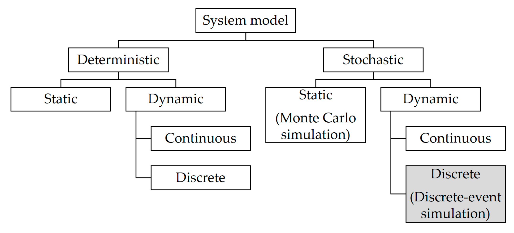
In general, a model intended for a simulation study is a mathematical model. Mathematical model classifications consist of deterministic (input and output variables are fixed values) or stochastic (at least one of the input or output variables is probabilistic); static (time is not taken into account) or dynamic (time-varying interactions among variables are taken into account), Figure 1. Typically, simulation models are stochastic and dynamic [10]. Based on system specification formalism, Kelton and Law [10] categorized dynamic models into two types, discrete and continuous. A discrete model changes instantaneously in response to certain discrete events. A continuous model is based on differential equations and attempt to quantify the changes in a system continuously over time in response to controls. From now on, the term model refers to the stochastic discrete model (the highlighted box in Figure 1). The next section presents a set of steps that should be followed in a simulation study.
2.2. Steps in a Simulation Study
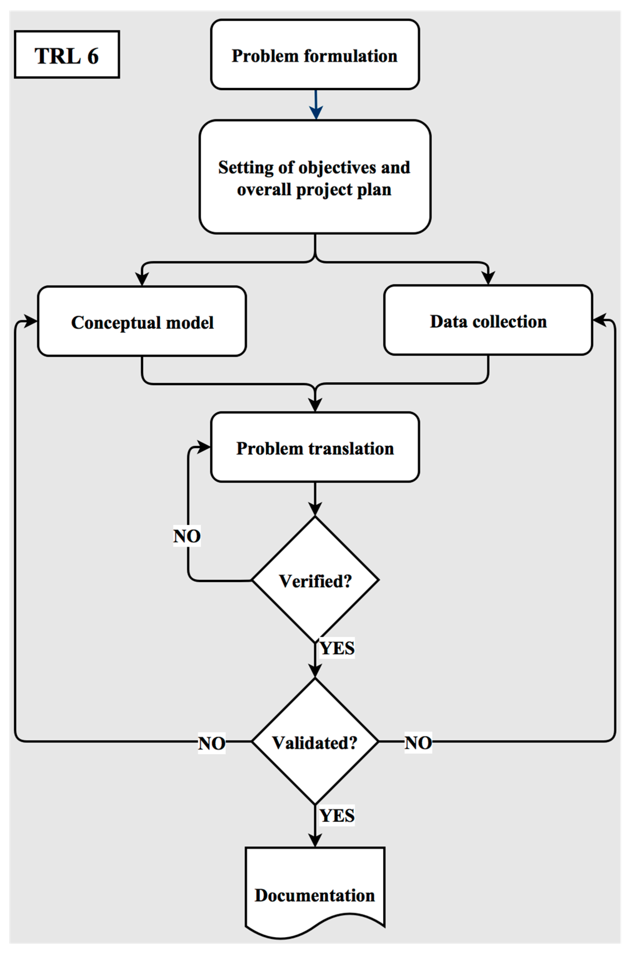
Figure 2 presents a set of steps that will be followed in this study for developing a simulation model, designing experiments, and performing simulation analysis [11].
- Problem formulation: The statement of the problem must provide the description of the purpose for building the model.
- Setting of objectives and overall project plan: The defined objectives indicate the questions that are to be answered by the simulation study. Different scenarios that will be investigated should be included in the project plan.
- Conceptual model: The system under study is abstracted by a conceptual model. In this paper, the conceptual model is a series of logical relationships concerning the components (e.g., excavators, spreaders, conveyor belts, etc.) and the structure (system topology) of the case study.
- Data collection: This stage includes tasks of gathering as much data as possible about the system under study. The model parameters and input probabilities to be used in the model will be defined. Model building and data collection are shown as contemporaneous in Figure 2. The simulation modeler can construct the model while data collection is progressing.
- Model translation: The constructed conceptual model in Step 3 is converted to an operational model. This step can be carried out using simulation software like Arena® [12]. The main tasks in this phase are the coding, debugging, and testing the operational model.
- Verification of the model: This stage compares the output results of the operational model with those that would have been produced by a correct implementation of the conceptual model.
- Validation of the model: This stage compares the outputs of the verified model with the outputs of the real system. It determines that the conceptual model is an accurate representation of system under study. If the system under study is an industrially relevant environment, in this step, TRL 6 will be achieved.
- Documentation: All necessary information with the results of the analysis step should be documented.
It should be noted that the aim of this study to achieve TRL 6. This paper is organized in a way that all steps (to achieve TRL 6) are discussed in detail by implementing them in two case studies. However, to understand the theory behind some steps, the following section elaborates more about the verification and the validation steps.
2.3. Verification, Validation, and Evaluation Measures
One of the most difficult problems facing a simulation analyst is that of trying to determine whether a simulation model is an accurate representation of the real-world system. This section presents definitions, techniques, and steps of verification and validation [10].
- Verification: a determination of whether the conceptual model has been correctly translated into a computer program.
- Validation: a determination of whether a simulation model is an accurate representation of the system.
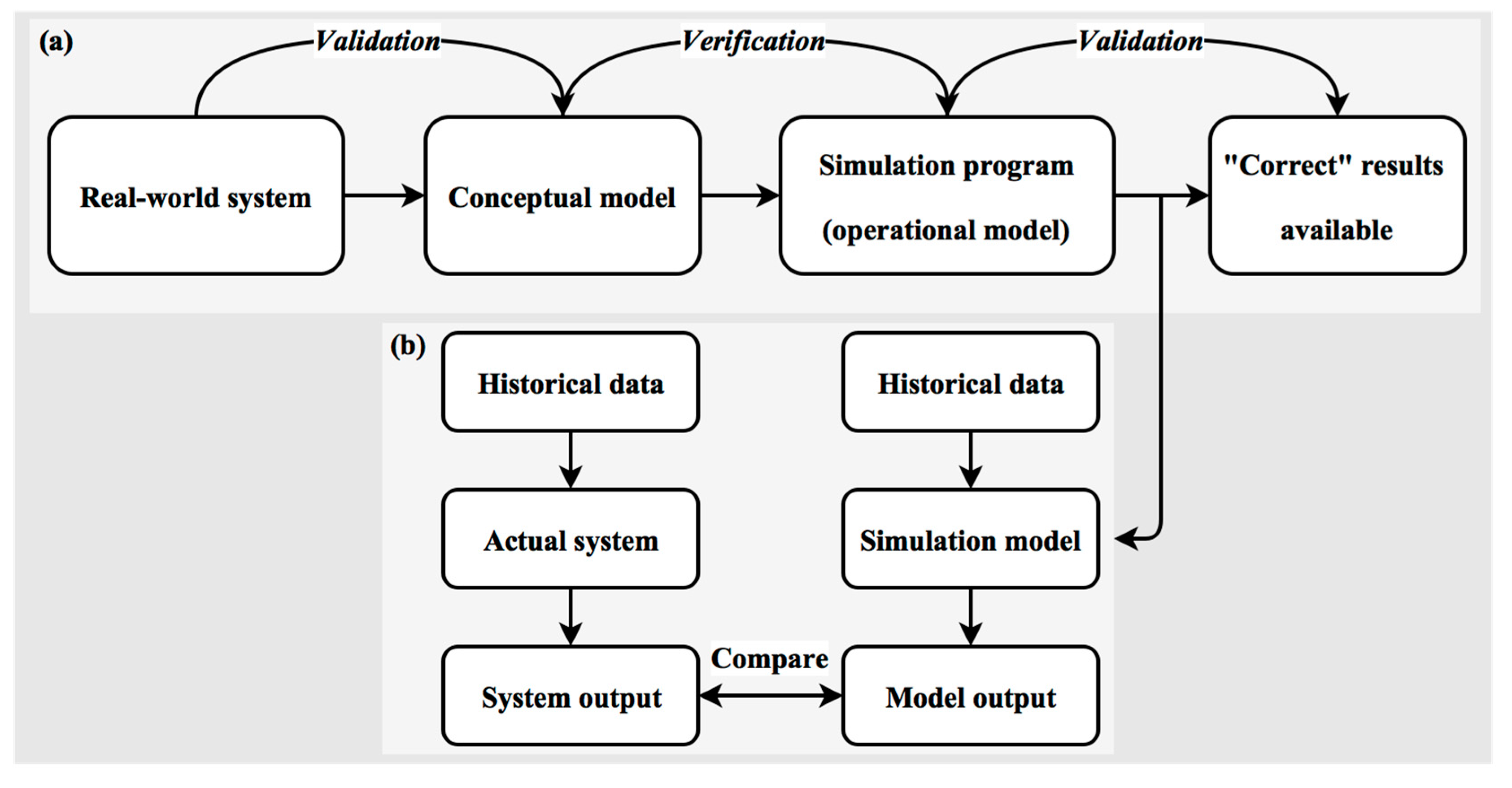
The chronological relationships of the validation and the verification are shown in Figure 3. The rectangles in part (a) of the figure represent states of the system under study, the solid horizontal arrows correspond to the actions necessary to move from one state to another, and the curved arrows show where the two major concepts are most prominently employed. The whole calibration process is mostly a trial-and-error procedure.
The most definitive test of a simulation model’s validity is to establish that its output result closely resemble the output result of the actual system. If the two sets of results compare “closely,” then the model of the existing system is considered “valid”. Part (b) in Figure 3 shows the applied approach in this study. The model is then modified so that it represents the proposed system. The greater the commonality between the conceptual model and real-world system is, the greater our confidence in the proposed model [10].
In this study, quantitative techniques are used to compare the output results of the simulation model with output results of the real system. Following evaluation measures are defined: bias, average deviation, and relative error.
- Bias: refers to the tendency of a measurement process to over- or under-estimate the value of a population parameter. The bias can be defined as the sum of differences between all predicted and actual Key Performance Indicator (KPI) values over all n predicted time intervals:
- Average deviation: is one of several indices of the prediction error. Within this study, it is defined as the mean absolute deviation between all predicted and actual KPI-values over all n predicted time intervals:
- Average relative error: the relative error is the absolute error (average deviation) divided by the magnitude of the actual value. Within this study, it is defined as:
This section has attempted to provide a brief theoretical background relating to the simulation modeling process. The rest of the paper will demonstrate the practical application of the simulation modeling in the field of continuous mining systems. First, objectives are defined and then those objectives are attempted to be achieved in the two defined test cases.
3. Goal and Objectives
As stated earlier, this research aims to extend the developed simulation model by [4] to a new level (TRL 6) by implementing and validating it in two large coal (lignite) mines.
Achievement of this goal involves the following objectives:
- Define the problem to be studied, constraints, and the type of analysis to be performed;
- Abstract the system into a model described by the components of the system, their characteristics, and their interactions;
- Identify, specify, and gather data in support of the model;
- Extend the existing simulation model with respect to the new problem, model, and data structure;
- Embed the simulation model in a simulation platform;
- Design some experiments for the purpose of the verification and the validation of the simulation model;
- Analyze the simulation outputs to draw implications and make recommendations for problem resolutions.
Having defined the goal and the objectives, the paper will continue by stating the test cases and the framework, which is based on the steps of a simulation study, to achieve the objectives.
4. Practical Implementation
This chapter describes the framework of modeling, simulation, and validation of the simulation model of large continuous mining operations in detail. The proposed extended simulation model is intended to reproduce operational behavior in full-scale considering material management. For demonstration purposes, two case studies have been defined. The first case study is the Hambach mine and its main focus is on material management. The second case study is the Profen mine. In addition to material management, this case also focuses on coal quality management. The following section introduces the case studies.
4.1. Problem Statement
4.1.1. Case Hambach: Overburden Management
A schematic view of the Hambach mine is shown in Figure 4. In total eight BWEs have to be scheduled to serve continuously seven spreaders with waste material and two bunkers with coal. Waste materials at the Hambach mine are categorized in three types of mixed soils, mixed soils type1 (M1), dry mixed Soils type2 (M2T) and wet mixed soils type2 (M2N). Each BWE excavates either lignite or waste in terrace cuts and transfers materials to the face conveyor belt, which carries it along the bench to the main conveyor belt. All excavated materials of the eight benches are distributed to their destinations at the mass distribution center. Based on a predefined daily schedule, waste is distributed to the seven spreaders for dumping, and lignite is forwarded to two coal-bunkers. Table 1 shows the technical specifications of the BWEs.
The mine operates 24 h per day and seven days per week. Regular maintenance is carried out on weekly, monthly, and annually based schedules. During the regular maintenance or an unscheduled breakdown, the production process ceases on the bench.
Historical data show that next to scheduled maintenance, breakdowns of the equipment occur in a random manner. Due to the “in series” system configuration, equipment units feeding or are connected to the ceased equipment are blocked and set out of the operation while the maintenance is being done or the failure is being repaired. Furthermore, because of the multi-layer nature of the deposit, changes from one material type (e.g., M1) to another material type (e.g., M2N) happen very frequently. Each time a material change takes place, the BWE stops excavating.
In summary, the system shows a stochastic behavior that is based on the randomness of significant system constituents and operations. The combined effect of frequent changes in extracted materials and random equipment breakdowns, makes the prediction of the exact material flow rate at any given future time span as a major source of uncertainty.
4.1.2. Case Profen: Production Efficiency and Coal Quality Management
Figure 5 shows the extraction system of the Profen mine. It consists of six excavators, two spreaders, and a coal-bunker. An overview of specifications of the equipment can be found in Table 2. The excavators have to be scheduled with the following operation details:
- The excavator Bg. 1580 extracts only waste (sand, gravel, and clay) and is connected to the spreader Abs. 1104.
- The excavators Bg. 1511 and Bg. 1553 can send the extracted materials to the all defined destinations, (the coal-bunker, the spreaders Abs. 1112, Abs. 1104).
- The excavators Bg. 351, Bg. 1541, and Bg. 309 extract coal and waste and have access to the spreader Abs. 1112 and the coal-bunker.
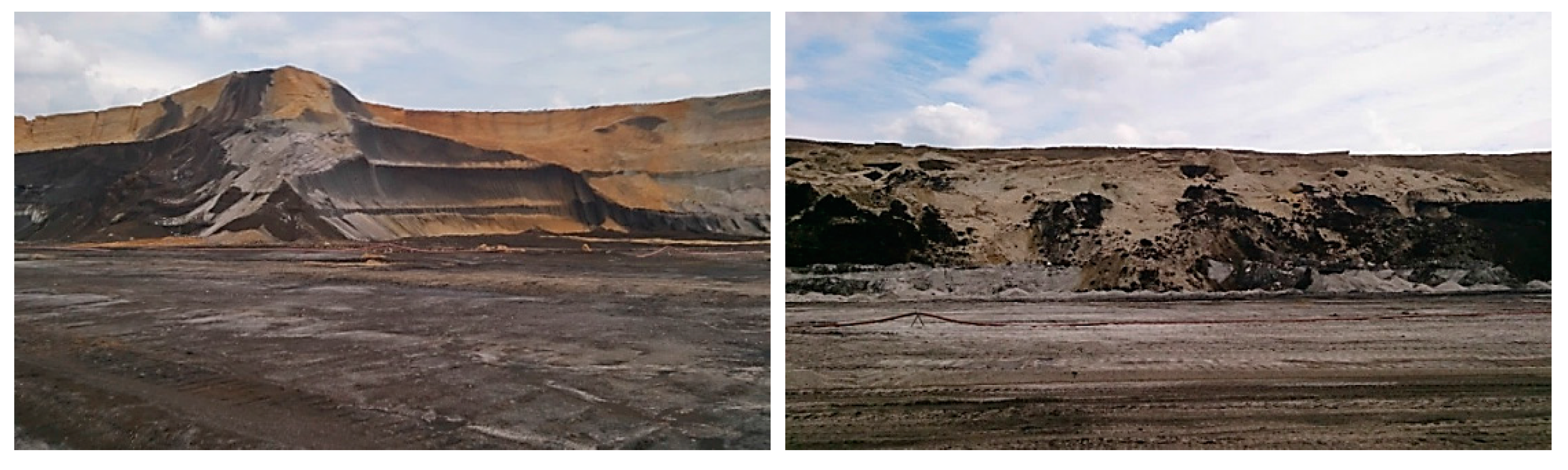
In this case, challenges originate from geological uncertainty associated with the detailed knowledge about the coal deposit as well as from unscheduled breakdowns of equipment as an internal factor. As an illustration, Figure 6 shows the difficult geology in the Profen mine that affects the deliverable coal quality and quantity. As part of the RTRO-Coal, Yueksel et al. [13] quantify geological uncertainty of the deposit using conditionally simulated realizations. They apply Sequential Gaussian Simulation method (SGS) to create the realizations. This paper uses their output result as the reserve block model. It includes an average type estimated model using Ordinary Kriging and 25 realizations of the deposit.
Three different coal including power plant coal 1 (KK1), power plant coal 2 (KK1), and dust coal (SK) can be extracted in the Profen mine. The features of the different coal types are given in Table 3. Coal quality control is performed via an online sensor measurement (RGI) and lab analysis. The online sensor is located on the conveyor 61 and measures ash and water content on a minute time interval. The most accurate measurement is done in a laboratory on samples that are taken from train cars leaving the stock/blending yard toward customers.
To emphasize the effect of geological uncertainty, Figure 7 shows the historical data about the ash content of delivered trains to a power plant. As can be seen, there are three different values; the average value of extracted blocks based on the estimated block model (magenta line), the online sensor measurement (blue line), and the laboratory measurement (green line). The lab measurements (which are called the reality in this paper) show a significant fluctuation compared to the estimated model. In addition, systematic deviations over longer time spans can be detected. These observations emphasize the necessity of accounting for the geological uncertainty when forecasting the coal quality by the mine simulator.
4.2. Conceptual Model of Continuous Mining Systems
The process of a continuous mining system can be divided into three sub-processes, see Figure 8. The operation starts with the excavation of materials by BWEs. It continues by the transportation of the extracted materials from mining benches to dumping benches or coal stockpiles. The transportation process includes a network of conveyor belts consisting of face conveyor belts, main conveyor belts, and a mass distribution center. Finally, lignite is stacked at the stockpile or waste materials are dumped at the waste dump.
The extraction and the transportation processes of materials can be emulated in a combined discrete-continuous stochastic environment. This provides the possibility to recreate the deterministic and/or random occurrences of events such as operating stoppages, which are caused by unavailability of spreaders or conveyor belts, equipment failures, and preventive/corrective maintenance activities.
The software selected to implement the simulation model is Rockwell Arena® 14.5 [12]. Arena® allows closely reproducing the behavior of the complex real systems with complicated decision logic [10]. Furthermore, KPIs will be used to evaluate the success of the simulation model. KPIs should be defined based on the target of simulation and optimization process. A KPI is a measurable value that demonstrates how effectively a simulation model is achieving the defined objective. Generally, for the introduced system, the quality, the quantity, and utilization of equipment are the major performance metrics. More details about the mathematical formulation of the evaluation function and the parameters of the KPIs to be evaluated are discussed in Shishvan and Benndorf [5].
Based on the different focus points of two case studies, the measured KPIs are as follow:
- Case Hambach: The quantity and the utilization KPI will be measured.
- Case Profen: All three KPIs will be measured.
4.3. Data Collection and Modeling of Stochastic Behavior
This section highlights the data that are required for building the simulator. The data are divided into three major groups including process related, elements related, and geological data, see Table 4. In our case studies, the process related and geological related data were easy to obtain. At the very beginning step, these data are provided by the both industrial partners. Fortunately, both mines have their own an SQL-based database. The elements related data can be extracted from their databases. They keep almost all operational data including:
- Any data that is related to the production process, e.g., amount of waste or coal and quality parameters of the delivered coal to different customers;
- Any data that is related to the breakdowns of equipment, e.g., at what time the failure happens, what is the root cause, and the duration of the failure (i.e., the repair time).
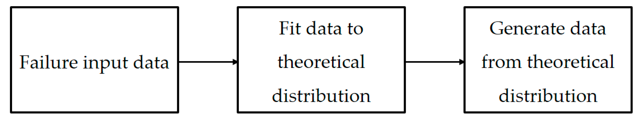
The first group of data will be used to verify/validate the simulation model. Among the second group, in this study, mechanical, electrical, conveyor system, and operational failures are encountered to be the most crucial failures. The historical data of these failures are processed as is shown in Figure 9. The analysis involves the identification of theoretical distributions that represent the input data. Arena® software facilitates the identification process by the Input Analyzer tool. After the theoretical distributions are fitted to the data, then any data values from the theoretical distributions may represent the failure behaviors. However, a possible weakness of this approach is that a theoretical distribution may periodically generate an unusual value that might not actually ever be present in the real system. This issue will be elaborated in the validation section with an example.
4.4. Model Building—Problem Translation
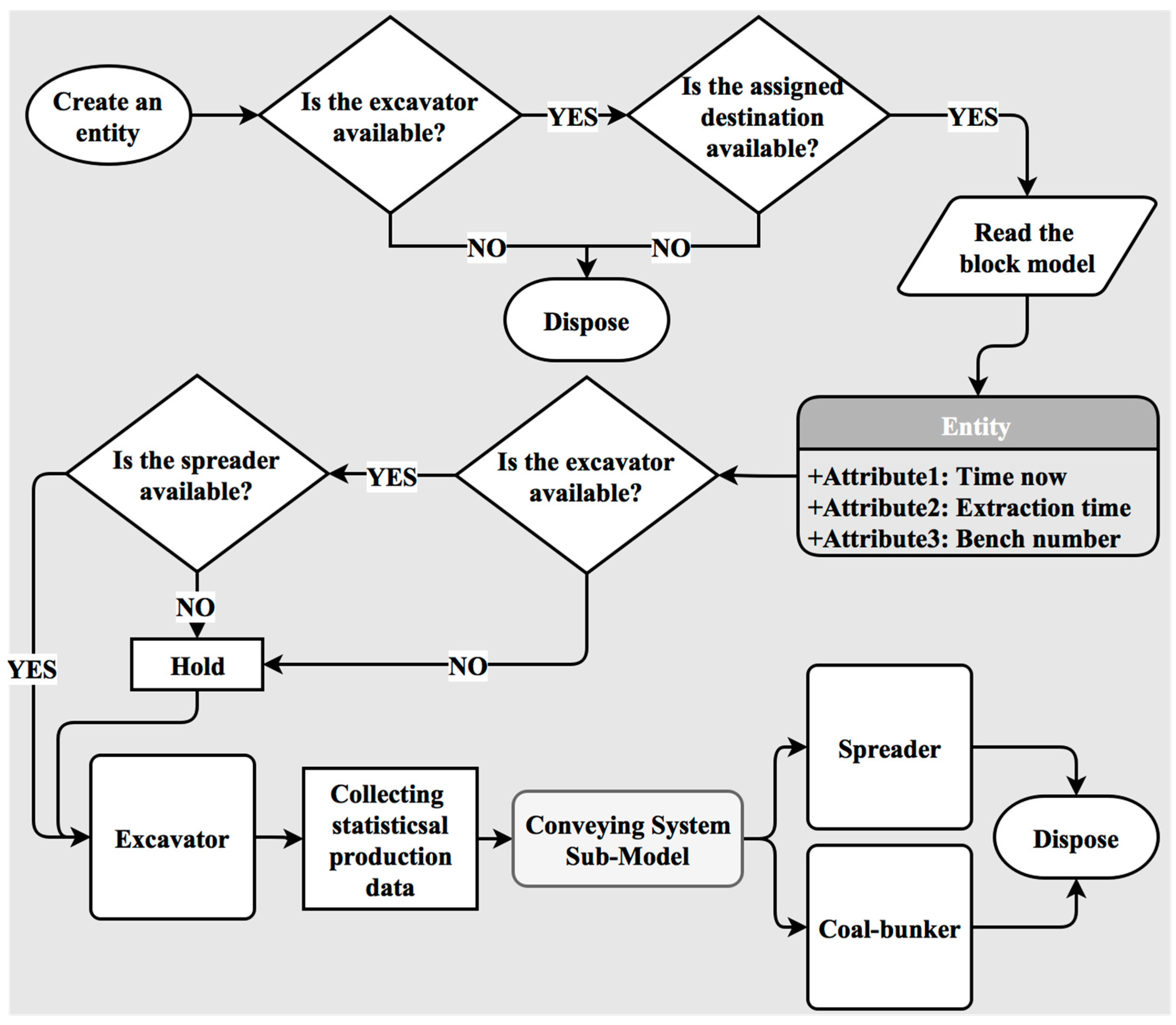
The main logic is designed based on the pervious sections, the conceptual model of a continuous mining system and the design of the model. Its flowchart is created and shown in Figure 10. In summary, a simulation begins with creating entities at minor intervals. As an entity arrives into the system statuses of the assigned excavator and spreader are checked. In case of unavailability of one of them, the entity is disposed at the very beginning step. If both are active, it reads the data file and assigns the values to the correspondence attributes. These attributes consisting of excavator number, bench information, conveyor belt number, block number, material type, volume, quality parameters, and the destination of the entity. Based on the material type, other type of attributes such as “time now” and “extraction time” are assigned on the way to the excavator. An entity has an “extraction time” attribute that corresponds to the delay that the entity should have in the excavator (a resource module in Arena).
The amount of the delay is equal to the time, if the excavator excavates the same amount of material in the reality. So, entity’s extraction time can be calculated using Equation (4) (the unit is minutes):
It should be noted that a “seize, delay, and release” resource module is used to imitate the excavation operation in the model. With this in mind, if the excavator and the spreader are still active, the entity is forwarded to seize in the resource module (the excavator). There, it has a delay as much as the extraction time attribute. After releasing the entity from the resource module, some statistics are recorded such as total waste volume, the total volume of each material type, total coal tonnage entering the system, and the weighted average of quality parameters (e.g., ash, calorific value). Thereafter, the entity is transported using a network of conveyor belts. When it reaches its defined destination, either dump site or coal stockpile. It passes the defined resource module. Here, also, some statistics are recorded such as the amount of different dumped/stacked materials. At the end, the entity leaves the simulation model by a dispose module.
As mentioned earlier, the model keeps track of some variables of interest during the simulation run. These variables are written in a text file at any user-defined intervals.
4.5. Embedding the Simulation Model in a Simulation Platform
To achieve maximum flexibility of the simulation model and as a preparation for the next steps in the RTRO-Coal project, the mine simulator is embedded into a simulation platform. In this platform, the simulator is used to estimate the evaluation function. All the simulation preparation and post processing are done by several Python scripts, which are all controlled by the central controller script.
4.5.1. Simulation Platform Overview
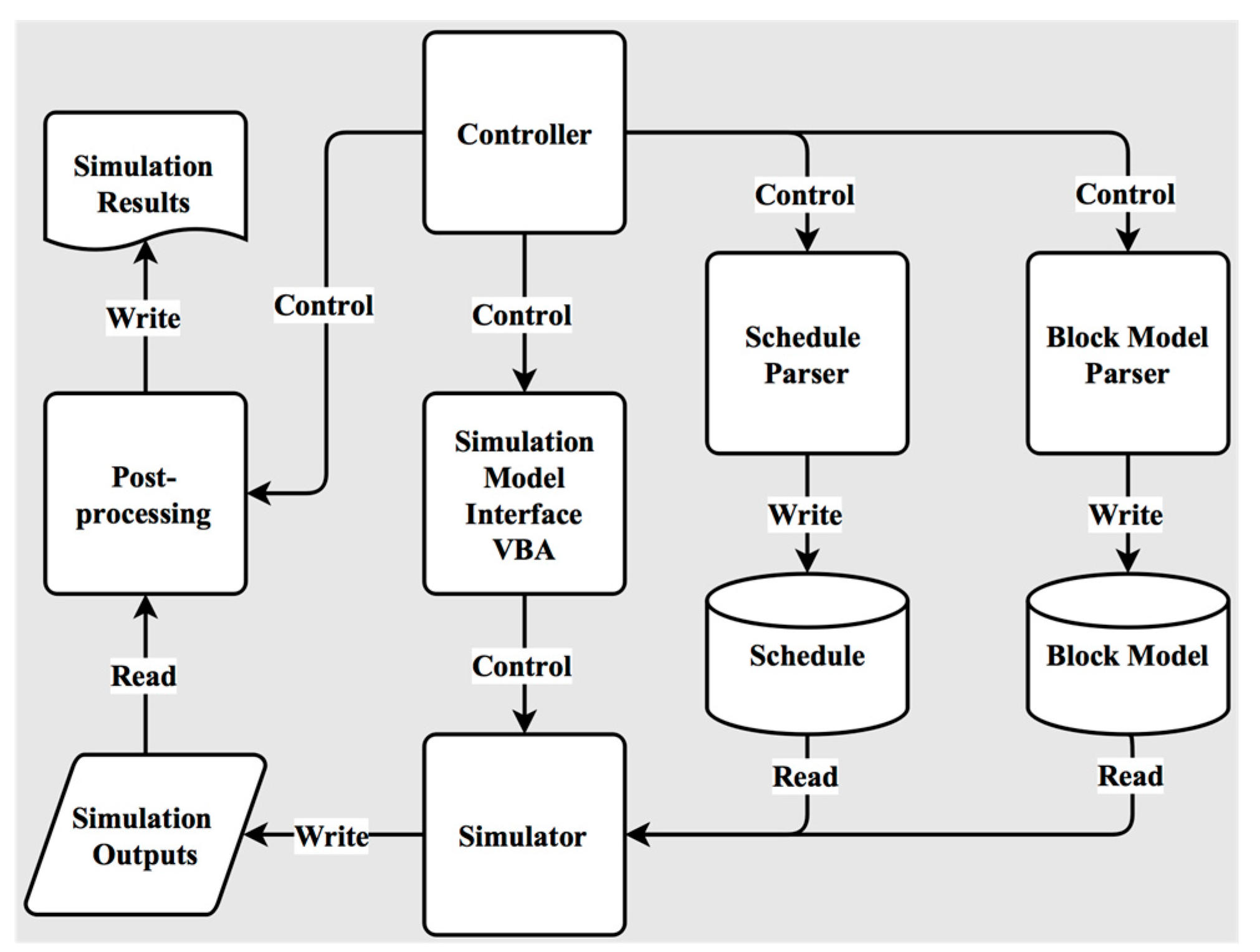
Figure 11 shows the simulation platform with its different processes. It also shows the relationship that processes have with each other. There are three relationships:
Control: The process controls another process, either via calling it with command line arguments or by using a programming interface.
- Read: The process reads information from a file and uses this for its processing.
- Write: The process writes information or results to a file, which either can be read by another process or is meant as an output to the user.
The run of a single simulation can be described as four tasks, each containing their own subtasks that are often handled by different scripts, all initiated by the controller.
The flow of a simulation run:
- Simulation configuration
- ○
- The controller stores the date to be simulated and the output directory in a configuration file.
- Simulation preparation
- ○
- The controller creates or clears the simulation output directory.
- ○
- The block model parser selects the blocks to be used for the simulation and writes them to a database.
- ○
- The schedule parser creates a schedule based on the weekly/monthly schedule of the mine and writes the schedule to a database.
- Simulation run
- ○
- The controller calls the simulation model interface, which in turn instructs Arena to load the desired simulation model, reload the schedule data and then to run the simulation.
- ○
- Arena reads the block model and schedule data from the databases, runs the simulation and writes the output to the simulation output files.
- ○
- The controller copies the Arena output files to the output directory.
- Simulation post-processing
- ○
- The post-processing script generates the tables and figures that show the simulation results.
A process worth attention is the simulation model interface, which is situated between the controller and Arena. This process is required because there is no direct way to interact with Arena using for example the command line. Instead, the program relies on automation via Visual Basic for Applications (VBA), a Microsoft technology for creating interconnection between applications. This technology is not available in Python, thus the simulation model interface is written in Visual Basic and compiled as an executable that can be run from the command line with the relevant parameters. The VB script will wait until the simulation run is complete and then exit, at this point the controller knows that the simulation is finished.
4.5.2. Post-Simulation Processing of Results
There are four main files created by the Arena simulation process:
- Coal-bunker output for all excavators and replications, one line per entity;
- Waste dump output for all excavators and replications, one line per entity;
- Aggregated volume statistics per excavator;
- Detailed activity log of excavators.
The coal and waste files contain the important parameters for each entity that exits in the system, as well as the time at which it does this and the replication number. The processing of these files contains the following steps:
- split the data per replication and resample the different entities,
- sum them up by day (for an example),
- determine the weighted average of quality parameters, and
- write the values in a file with the following order: replication, date, values.
The post-processing then creates various plots that give an overview of the performance of the simulation. For coal and waste, both the mean production and the uncertainty of the daily production are plotted. The uncertainty is used as a P10 minimum and P90 maximum value. These values are obtained by sorting the values of the different replications ascending and then taking the value at index N*0.1 for the P10 and N*0.9 for the P90, where N is the total number of replications.
For the quality, the plotting is slightly different. Since there are 25 different simulated ash values, the calculation will take the value of quality simulation for replication . The P10 and P90 value are then calculated in the same way as for the production volume. The estimated ash values is also plotted to compare the values.
4.6. Design of Experiments for Validity Test of the Case Studies
To evaluate the validity of the simulation model, a set of numerical experiments was designed. The strategy for designing experiments follows three major objectives. The first objective is to show that the simulation model reproduces observed data of the real system, when historic deterministic input is provided. The second objective is to demonstrate the strength of the simulation model when ‘breakdown behavior’ as a stochastic component is added, (the utilization KPI). The third objective is to quantify the effect of geological uncertainty and reconcile its results against measured KPIs observed in the reality. The first two objectives are pursued in the both case studies but the last objective is sought only in the case Profen. With these in mind, experiments are designed as follows:
- Experiment 1: Run the simulation model without stochastic components
- ○
- The input reserve block model is derived from actual measured data and all parameters such as working schedule, failures, and excavation rates are taken as historically performed as deterministic values.
- ○
- The target of this experiment is to verify the output of the simulation model against with what exactly happened in the mine during the time horizon considered.
- Experiment 2: Run the simulation model with stochastic component “breakdown behavior”
- ○
- The reserve block model is kept as in Experiment 1 and it represents the reality. In this experiment, theoretical distributions for predicting unscheduled breakdowns of equipment are added to the model as stochastic components.
- ○
- The target of this experiment is to test the reliability of the model in predicting downtimes. The utilization KPI is measured.
- Experiment 3: Run the simulation model with stochastic component “breakdown behavior” and “reserve block model”
- This experiment is designed for the quantification of geological uncertainty in the Profen mine. After being certain that equipment failure models are good enough, the stochastic input “reserve block model” is added to the simulation model. In total, there are 26 different reserve block models (different possible values for ash content) as mentioned earlier.
4.7. Results
The following section presents results of the experiments. It should be noted that for both case studies, three months of production data are used to validate the simulation models. However, only the part of the results that emphasizes the practical implementation issues and challenges are presented.
4.7.1. Case Profen
Experiment 1: Simulation Model without Stochastic Components
Table 5 provides the summary statistics of simulated and actual production data with the calculated evaluation measures. Closer inspection of the table shows that the difference for the coal is very close to zero and no difference greater than 4% was observed. In addition, it is apparent that the average relative error per day displays higher values. These values are rather counterintuitive. A possible explanation for this is due to high variability, there are significant deviations on a short-term (daily) basis. However, on average, the prediction of coal is good.
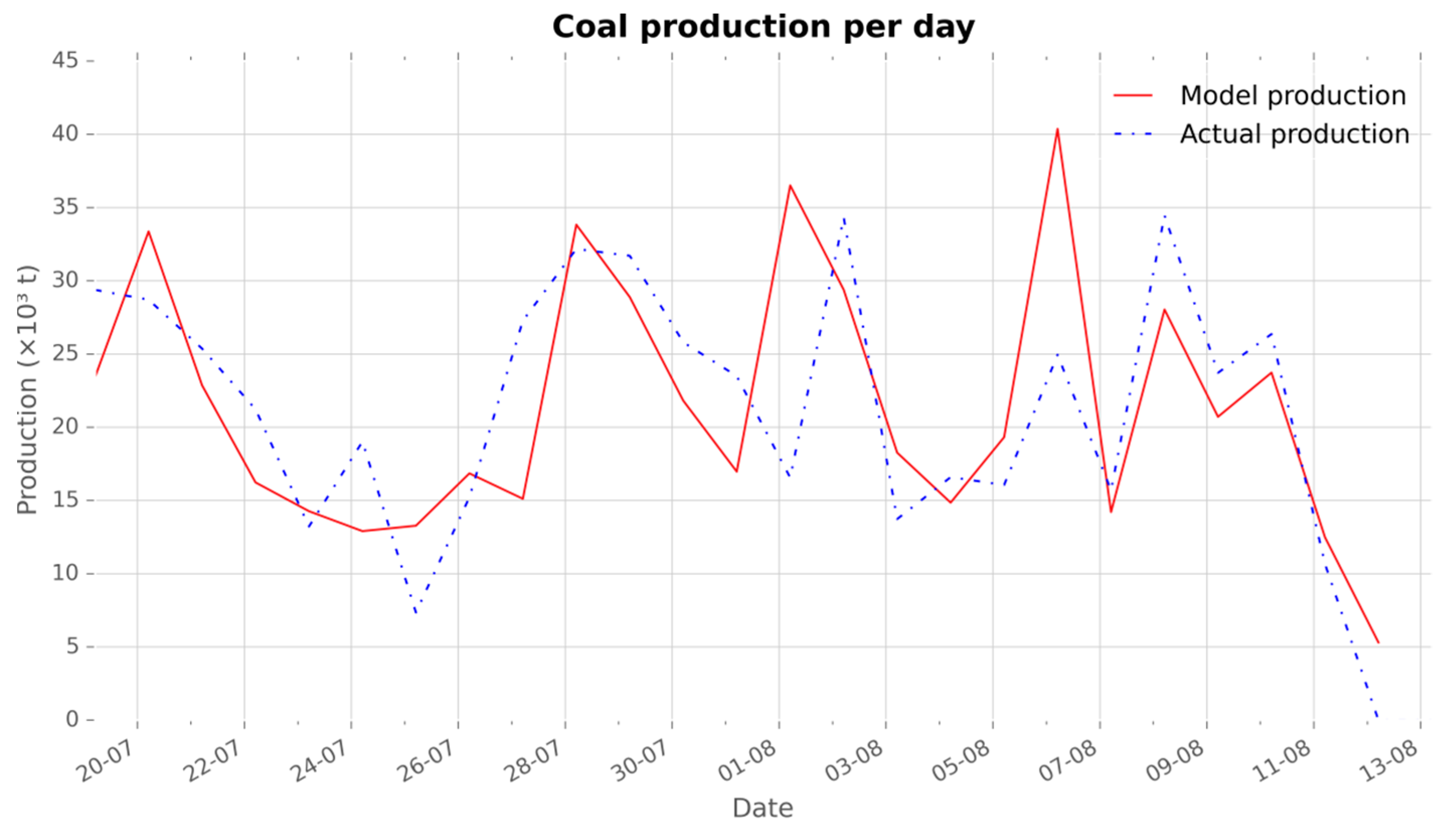
Furthermore, for the given time horizon, the graphs of the daily production of coal and waste are shown, respectively, in Figure 12 and Figure 13. What stands out in the figure is that the output of the simulation model (model production) is well correlated with the actual production of the mine. Taken together, these results indicate the verification of the simulation model with all deterministic inputs against the real system.
Experiment 2: Simulation Model with Stochastic Component “Breakdown Behavior”
In this experiment, theoretical distributions of failure models related to equipment breakdown behaviors are added to the simulation model. The number of simulation replications was set to 20 as recommended by Shishvan and Benndorf (2016) [4]. The obtained results are presented in Table 6. It is clear from the table that following the addition of the stochastic components, significant increases in the average deviations and average relative errors were recorded. However, increments in the differences (sum of over/under production in the given time horizon) were not statistically significant (less than 2%). Further investigation showed that an unusual long breakdown of one piece of equipment happened in situ during the study time horizon. Not surprisingly, the historical failure data show that the probability of an occurrence of such a long lasting failure is very low. Nevertheless, such circumstances are unavoidable due to the stochastic nature of unscheduled breakdowns.
Additionally, the daily production graphs of coal and waste are presented, respectively, in Figure 14 and Figure 15. The dashed-line shows the actual production, the solid-line shows the average of simulation replications, and the dark shadow part demonstrates the predicted range of uncertainty (area between 0.10 and 0.90 quantile) introduced by the stochastic breakdown behavior. The single most striking observation to emerge from the figure is the negative correlation between the simulated and the actual production in two parts of the graphs. As discussed earlier, an unusual long breakdown happens in the beginning of the time horizon (21.07–25.07), which is not predicted by the failure models. Therefore, the simulation continues the production process while in the reality the production is decreased. In addition, a closer look at the graphs shows another negative correlation at the end of the time horizon. This behavior surfaced mainly in relation to first issue as well. For that reason, it is completely a natural behavior if at the end of the period a shortage is observed due to the overproduction at the beginning. The argument is valid for both coal (Figure 14) and waste (Figure 15) graphs in the figure. Overall, the average of simulations and the actual production are positively correlated. There are some differences, but differences are inside the uncertainty range.
The second objective of this experiment is to demonstrate the reliability of the simulation model in terms of the utilization KPI. Table 7 summarizes the utilization KPI predicted by the simulation model. Table 8 presents the actual utilization. Differences between the actual and the simulated utilization are given in Table 9. In the presented tables, the status “Busy” means the excavator is digging materials, “Failed” means the excavator is stopped working (e.g., due to a failure), “Idle” means the excavator is neither digging nor failed (e.g., transportation), and “Inactive” means the excavator is not working (e.g., due to the periodic maintenance or planned downtime).
The range of differences for busy status (operating time) varies between −5.7% and 4.7% in the time horizon of three months. The simulation model of a continuous mine is a complex problem and there are a lot of influencing factors. Statistically, this range could be represented as an acceptable range. These results underline the validity of probability distributions that are used for the prediction of unscheduled breakdowns. However, it should not be forgotten that cases such as the breakdown of Bg. 1553 could happen, though they represent outliers. They are unavoidable and sometimes unpredictable due to the stochastic nature of unscheduled breakdowns.
Experiment 3: Simulation Model with Stochastic Component “Breakdown Behavior” and “Reserve Block Model”
The third experiment is the most comprehensive test. The summary statistics are summarized in Table 10. As it can be seen, the difference between the simulated and the actual production are 10.24% for coal and 1.54% for waste. In this experiment, differences are higher when comparing to the pervious experiments. This is expected due to the uncertainty associated with the reserve block model. The sum of the produced coal and waste shows the difference of less than 3%, which is statistically an acceptable deviation.
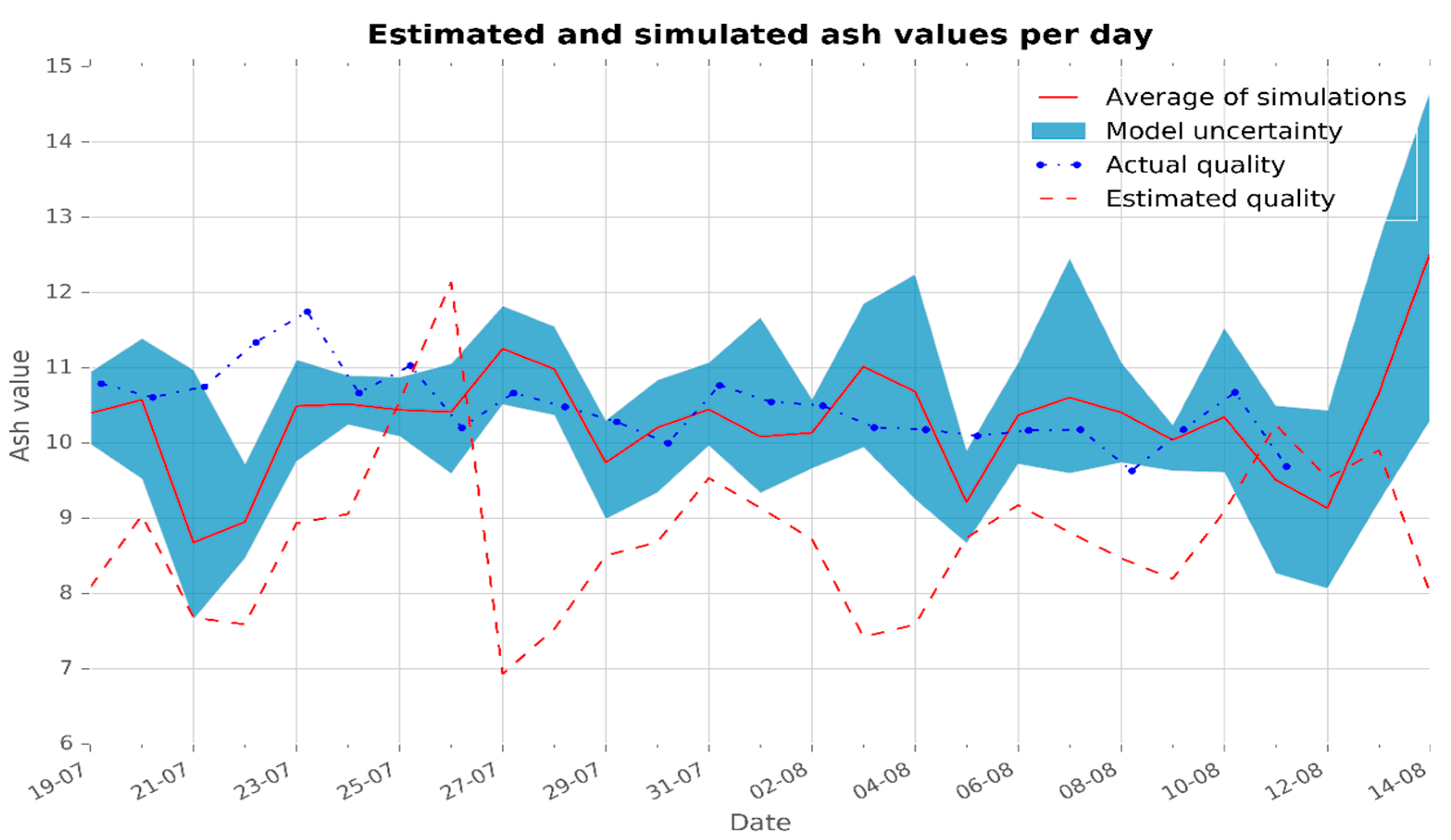
To quantify the effect of geological uncertainty the average daily ash values are compared in Figure 16. The blue dashed-dot-line shows the ash value of actual production, the red dashed-line demonstrates ash values of the estimated model, and the solid red line presents the average ash values of the simulations (realizations). The predicted range of uncertainty is illustrated by a dark shadow cloud in the graph. It is clear from the figure that the estimated model and the actual production are not well correlated. The estimated model has a tendency to underestimate ash values. This issue was discussed in the problem statement section.
What is striking about the graphs in Figure 16 is that the actual production data are well covered by the predicted range of uncertainty. Only at the beginning of the time horizon, some parts are outside of the range. As discussed earlier, a breakdown that is happened and not captured by the failure models is the reason for this phenomenon.
Similar to the previous experiments the daily production of coal and waste are shown, respectively, in Figure 17 and Figure 18. From the graphs below a relatively good match can be seen. However, the existed inconsistency in the reserve block model causes some deviations. It can be seen that the quality of the historical data is the key factor to achieve good results.
Together these results provide important insights into the verification and the validation process of the simulation model of the Profen mine. Some important points can be:
- A good prediction over long time frames.
- Deviations were seen on short scale due to geological uncertainty.
- The occurrence of seldom events may not be well captured in simulation experiments.
- In this case, for practical application, the model input would have to be adjusted according to the actual situation (e.g., equipment down for some timeframe) and iteratively re-run it.
Finally, an important implication emerged from these results is that the simulation model can effectively be used as a decision making tool. Impacts of the different decisions (e.g., different task schedules) can be assessed by the simulation model. The next section presents the validity test results of the Hambach case as a second case study.
4.7.2. Case Hambach
Experiment 1: Simulation Model without Stochastic Failure Models
Summary statistics of a monthly production with the calculated evaluation measures are presented in Table 11. What stands out in the table is that the total deviation is about 100,000 m3, which is only 0.47% of the total production. To explain better, the total theoretical capacity of the equipment of the Hambach mine is about 86,000 (m3/h). It denotes that the total deviation between the actual and prediction is slightly more than an hour of the production. Taken together, it can be seen that the simulation model imitates the reality with an acceptable precision.
Furthermore, the total shift-based production of the Hambach mine during the test’s time horizon is shown in Figure 19. The dashed-line shows the actual production and the solid-line presents the simulated production data. The presented graphs illustrate that the simulated follows the actual production data with some deviations. As explained in the previous section, these deviations occur due to the existence of some inconstancies in the reserve block model.
Additionally, for different material types (e.g., M1, M2T, etc.) shift-based production graphs are presented in Figure 20. Closer inspection of the graphs shows that, with Coal (f), as an example, there is analogous behavior between the simulated and the actual data. Overall, statistical measures such as the average deviation of about 27,000 m3 and the average relative error of 0.13% per shift indicate the verification of the simulation model.
Experiment 2: Simulation Model with Stochastic Failure Models
In this experiment, failure models are added to the simulation model. This experiment is specifically designed to show how reliable those models are. The summary and statistical measures of experiment 2 are presented in Table 12. Values in the simulated column of the table are the average values of 20 simulation replications. It is apparent that deviations are increased when comparing with the Experiment 1. This is due to the addition of the stochastic components into the simulation model. No significant difference between the actual and the simulated data is observed. The maximum difference occurs in the production of coal, which is equal to 2.9%. When considering the whole operation, a difference of 1.23% is recorded for a month of production. In a smaller scale, no difference greater than about 31,000 (m3) per shift was observed.
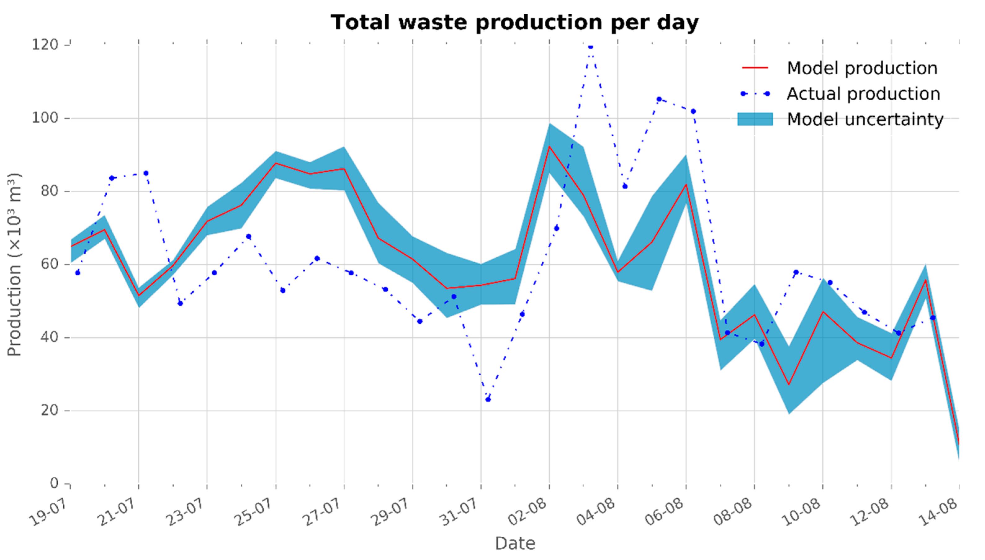
The total shift-based production for the given time horizon is presented in Figure 21. The dashed-line shows the actual production and the solid-line presents the average of simulation replications. Moreover, the dark shadow cloud is added to the graph as the predicted range of uncertainty (area between 0.10 and 0.90 quantile). From the figure, a well correlation between the simulated and the actual production data can be found. In addition, it is clear that the actual production is well covered by the shadow part.
Likewise, in Figure 22, a good correlation can be seen for the presented production data of different material types. However, it can be seen from this illustration that where there are a sufficient number of observations (Figure 22a–c,f), the actual and simulated values are well correlated, but where there are few data points, such as Figure 22d or Figure 22e, the error between the simulation model’s predictions and the actual data points is increased.
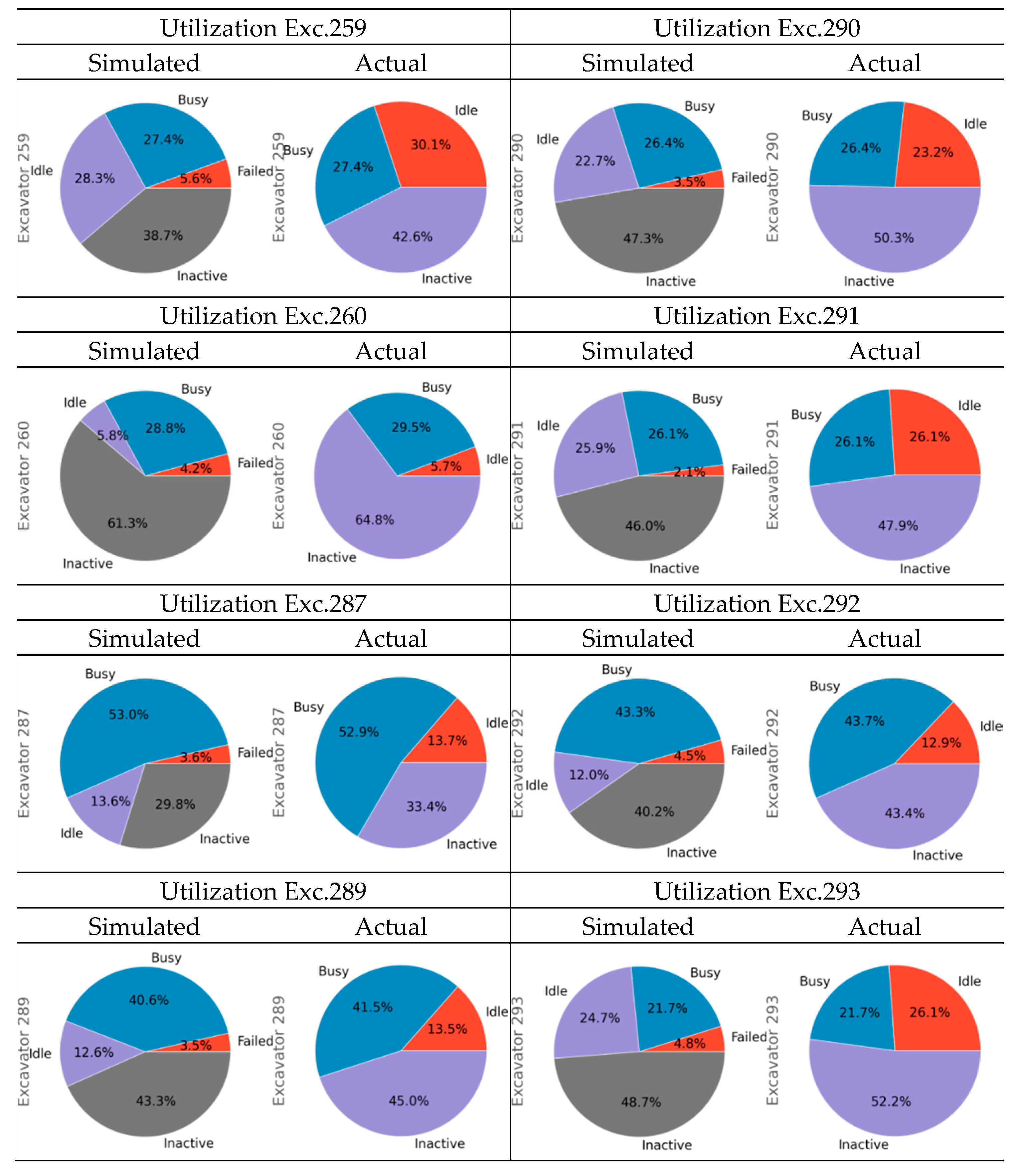
As stated earlier, the utilization KPI is measured in Experiment 2. The results are presented in the form of pie charts in Figure 23. The “Busy”, “Failed”, “Idle”, and “Inactive” statuses have already been defined in the previous case. For each excavator, two pie charts are given. One represents the actual utilization recorded at the mine and the other represents the simulated utilization by the simulation model. At the first glance, there are a number of similarities between the simulated model and the actual system. The most significant parameter that has to be very close to the reality is the percentage of the busy hours. In most of the cases (excavator 259, 290, 291, and 293), these percentages are same. For the other excavators, no differences greater than 1% were observed. For a better clarification, 1% difference in a month (744 h) refers to only 7.44 h difference. From these results, it can be inferred that the failure models are good enough to predict breakdown behaviors of the equipment.
To summarize this section, the results show that, first, the simulation models (both cases) are verified/validated against the historical data. Second, the developed simulation models are reliable when the failure models (for the purpose of prediction of downtimes) are added to the model. An implication that can be drawn from the results is the possibility of using the simulation modeling approach as an operational decision support. The proposed method can also be applied in other research areas such of waste management or recycling of material excavated from tunnels [15,16]. The next section concludes the main findings of this study.
5. Conclusions
Throughout this study, the developed simulation model by [4] has been extended to a new technology readiness level (TRL 6) by implementing it in an industrially relevant environment. A framework for modeling, simulation, and validation of the simulation model of a large continuous mine has been presented in detail. The framework was implemented in two large coal (lignite) mines. The case study approach was chosen to provide detailed illustrations of steps of a simulation study, implementation issues, and challenges in practical applications. A number of important practical implications emerge from this study:
- The quality of the historical data that are used for the calibration of the simulation model is very important.
- Experienced problem formulators and simulation modelers are crucial for a successful simulation study.
- The occurrence of seldom events (e.g., long breakdowns of equipment) may not be well captured in simulation experiments.
The second aim of this paper was to demonstrate the strength of the simulation modeling as an operational decision support for material management. The relevance is clearly supported by the current findings. The results indicate that a validated simulation model can be used to assess the impacts of different scenarios (e.g., different task schedules) in the mine. Based on the type of analysis and the measured KPIs, the best scenario among all can be executed in the reality.
As stated earlier, this study will serve as the basis for future studies in the RTRO-Coal research program. The next step will be the integration of the simulation modeling into a simulation-based optimization of short-term mine planning and operations control framework.
Acknowledgment
This research was supported by the Research Fund for Coal and Steel of European Union. RTRO-Coal, Grant agreement no. RFCR-CT-2013-00003.
Author Contributions
M. Soleymani Shishvan designed and performed the experiments. He also analyzed the data under the supervision of J. Benndorf. M. Soleymani Shishvan wrote the paper and J. Benndorf reviewed the paper before the submission.
Conflicts of Interest
The authors declare no conflict of interest.
Appendix A

Table A1.
Technology readiness levels defined by the European Commission [6].
Table A1.
Technology readiness levels defined by the European Commission [6].
| Technology Readiness Level | Description |
|---|---|
| TRL 1 | basic principles observed |
| TRL 2 | technology concept formulated |
| TRL 3 | experimental proof of concept |
| TRL 4 | technology validated in lab |
| TRL 5 | technology validated in relevant environment (industrially relevant environment in the case of key enabling technologies) |
| TRL 6 | technology demonstrated in relevant environment (industrially relevant environment in the case of key enabling technologies) |
| TRL 7 | system prototype demonstration in operational environment |
| TRL 8 | system complete and qualified |
| TRL 9 | actual system proven in operational environment (competitive manufacturing in the case of key enabling technologies; or in space) |
References
- Truong, T.H.; Azadivar, F. Simulation optimization in manufacturing analysis: Simulation based optimization for supply chain configuration design. In Proceedings of the 35th Conference on Winter Simulation: Driving Innovation, New Orleans, LA, USA, 7–10 December 2003. [Google Scholar]
- Jung, J.Y.; Blau, G.; Pekny, J.F.; Reklaitis, G.V.; Eversdyk, D. A simulation based optimization approach to supply chain management under demand uncertainty. Comput. Chem. Eng. 2004, 28, 2087–2106. [Google Scholar] [CrossRef]
- Benndorf, J.; Yueksel, C.; Shishvan, M.; Rosenberg, H.; Thielemann, T.; Mittmann, R.; Lohsträter, O.; Lindig, M.; Minnecker, C.; Donner, R.; et al. RTRO–Coal: Real-Time Resource-Reconciliation and Optimization for Exploitation of Coal Deposits. Minerals 2015, 5, 546–569. [Google Scholar] [CrossRef]
- Shishvan, M.S.; Benndorf, J. The effect of geological uncertainty on achieving short-term targets: A quantitative approach using stochastic process simulation. J. South. Afr. Inst. Min. Metall. 2016, 116, 259–264. [Google Scholar]
- Shishvan, M.S.; Benndorf, J. Performance optimization of complex continuous mining system using stochastic simulation. In Proceedings of the International Conference on Engineering Optimization (ENGOPT 2014), Lisbon, Portugal, 8–11 September 2014. [Google Scholar]
- European Commission. Technology Readiness Levels (TRL), Horizon 2020–Work Programme 2014–2015 General Annexes, Extract from Part 19; European Commission: Helsinki, Finland, 2014. [Google Scholar]
- Schmidt, J.W.; Taylor, R.E. Simulation and Analysis of Industrial Systems; RD Irwin: Homewood, IL, USA, 1970. [Google Scholar]
- Maria, A. Introduction to modeling and simulation. In Proceedings of the 29th Conference on Winter Simulation, Atlanta, GA, USA, 7–10 December 1997. [Google Scholar]
- Birta, L.G.; Arbez, G. Modelling and Simulation: Exploring Dynamic System Behaviour; Springer: London, UK, 2013. [Google Scholar]
- Kelton, W.D.; Law, A.M. Simulation Modeling and Analysis; McGraw Hill: Boston, MA, USA, 2000. [Google Scholar]
- Banks, J. Handbook of Simulation: Principles, Methodology, Advances, Applications, and Practice; John Wiley & Sons: Hoboken, NJ, USA, 1998. [Google Scholar]
- Rockwell Automation Technologies; Version 14.50.00000-CPR 9 SR 2; Arena Inc.: San Diego, CA, USA, 2012.
- Yueksel, C.; Benndorf, J.; Lindig, M.; Lohstraeter, O. Updating the coal quality parameters in multiple production benches based on combined material measurement: A full case study. Int. J. Coal Sci. Technol. 2017, 1–13. [Google Scholar] [CrossRef]
- Chung, C.A. Simulation Modeling Handbook: A Practical Approach; CRC Press: Boca Raton, FL, USA, 2003. [Google Scholar]
- Petitat, M.; von Allmen, K.; Burdin, J. Automation of rock selection and aggregate quality for reuse in tunnelling and industry. Geomech. Tunn. 2015, 8, 315–320. [Google Scholar] [CrossRef]
- Entacher, M.; Resch, D.; Reichel, P.; Galler, R. Recycling of tunnel spoil–laws affecting waste from mining and tunnelling/Wiederverwertung von Tunnelausbruchmaterial–Abfallrecht im Berg-und Tunnelbau. Geomech. Tunn. 2011, 4, 692–701. [Google Scholar] [CrossRef]
Figure 1.
System model taxonomy (reproduced after [10]).
Figure 1.
System model taxonomy (reproduced after [10]).

Figure 2.
Steps in a simulation study (reproduced after [11]).
Figure 2.
Steps in a simulation study (reproduced after [11]).

Figure 3.
The applied approach for validation process (Reproduced after [10]).
Figure 3.
The applied approach for validation process (Reproduced after [10]).

Figure 4.
Schematic overview of the production system of the Hambach mine.
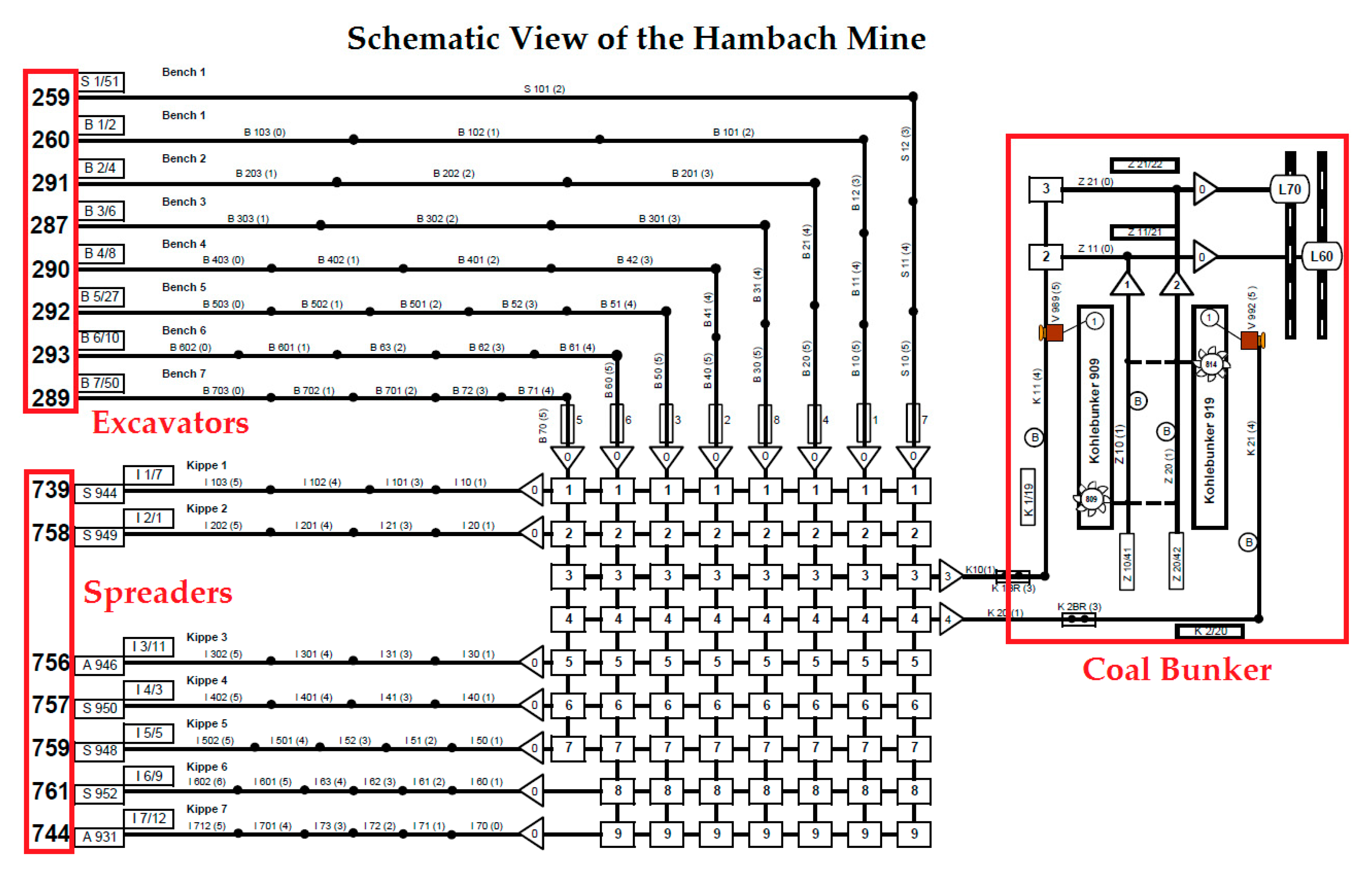
Figure 5.
Schematic overview of the production system in the Profen mine.
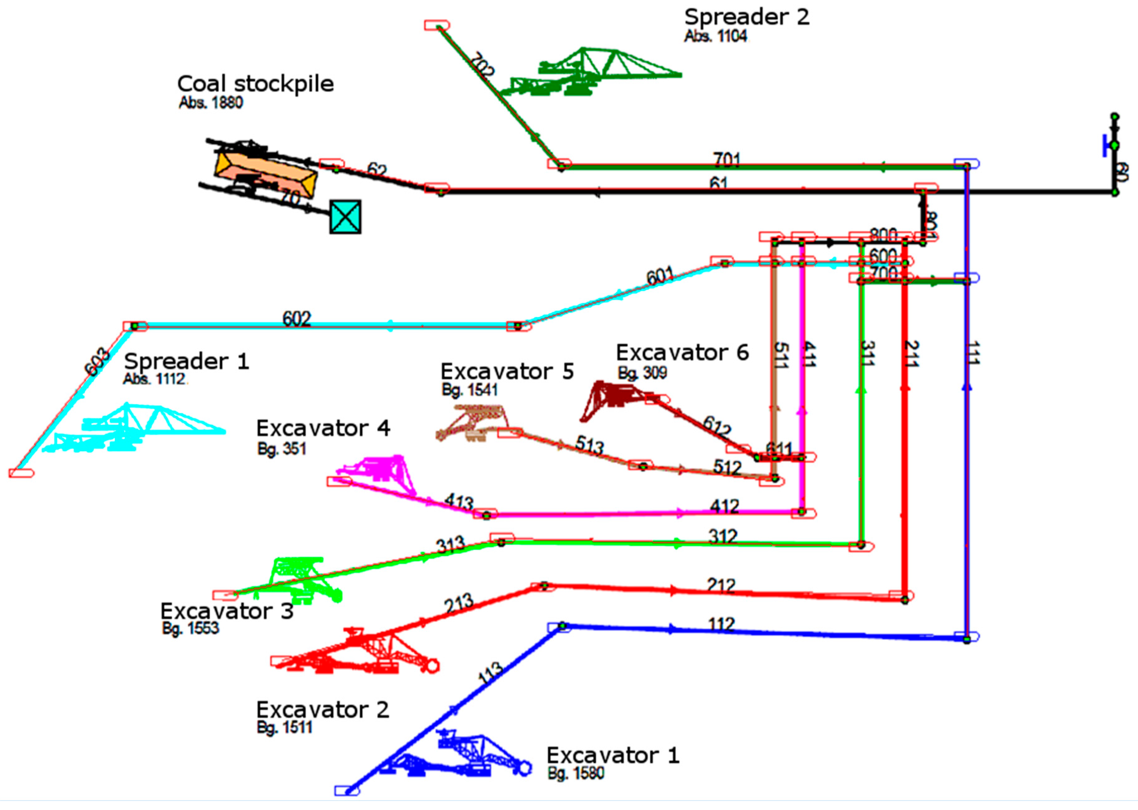
Figure 6.
Complicated geology in the Profen mine (second bench).

Figure 7.
Historical data of ash content of delivered trains to the power plants (provided by Mitteldeutsche Braunkohlengesellschaft mbH (MIBRAG).
Figure 7.
Historical data of ash content of delivered trains to the power plants (provided by Mitteldeutsche Braunkohlengesellschaft mbH (MIBRAG).
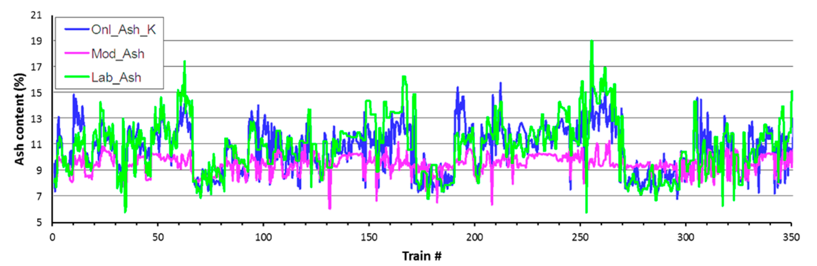
Figure 8.
The sub-process of the continuous mining system.

Figure 9.
Procedure of processing failure input data [14].
Figure 9.
Procedure of processing failure input data [14].

Figure 10.
Flowchart of the main logic behind the simulation model.

Figure 11.
Simulation platform diagram.

Figure 12.
Comparison of daily production of coal, Experiment 1.

Figure 13.
Comparison of daily production of waste, Experiment 1.
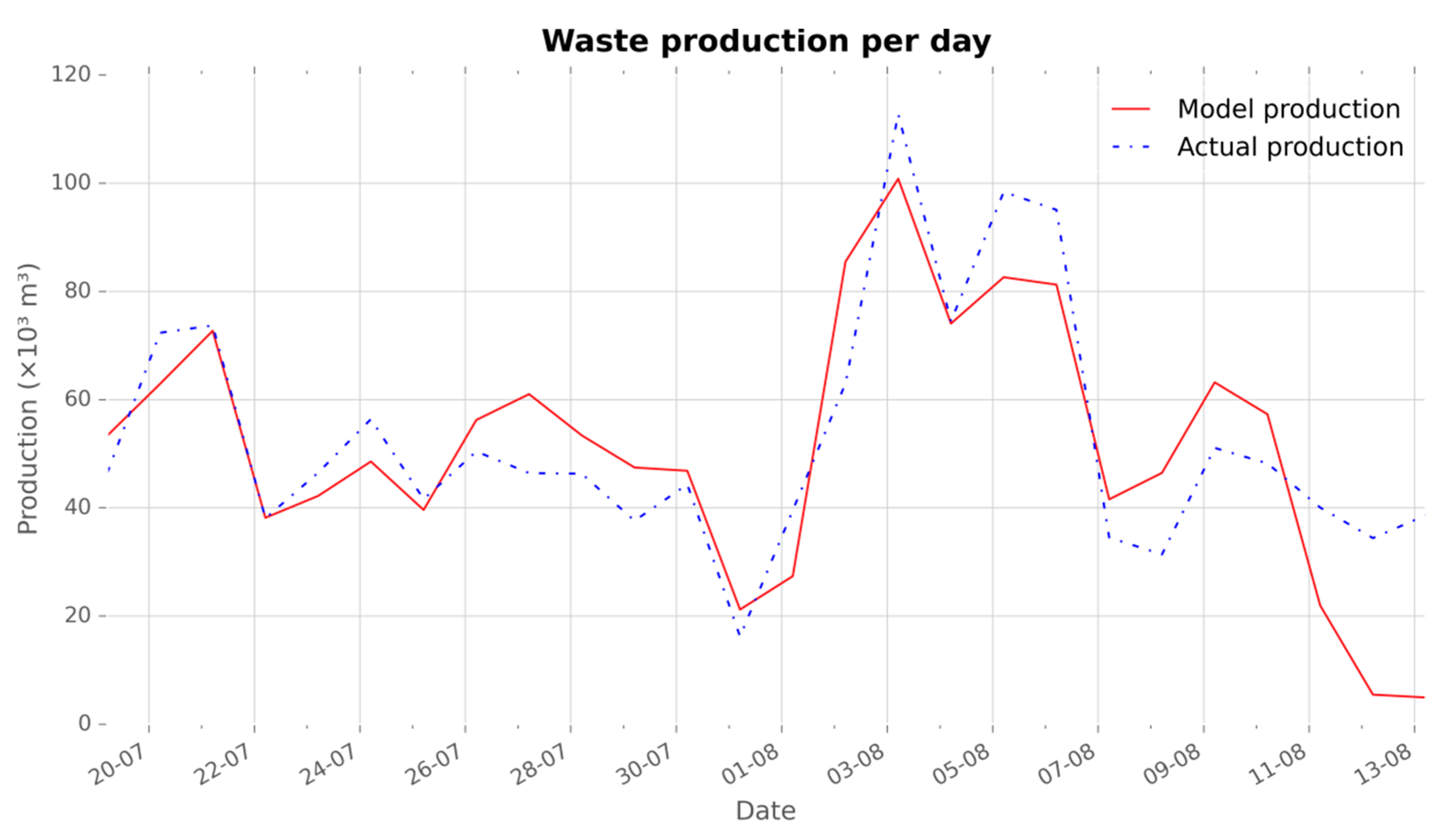
Figure 14.
Comparison of daily production of coal, Experiment 2.
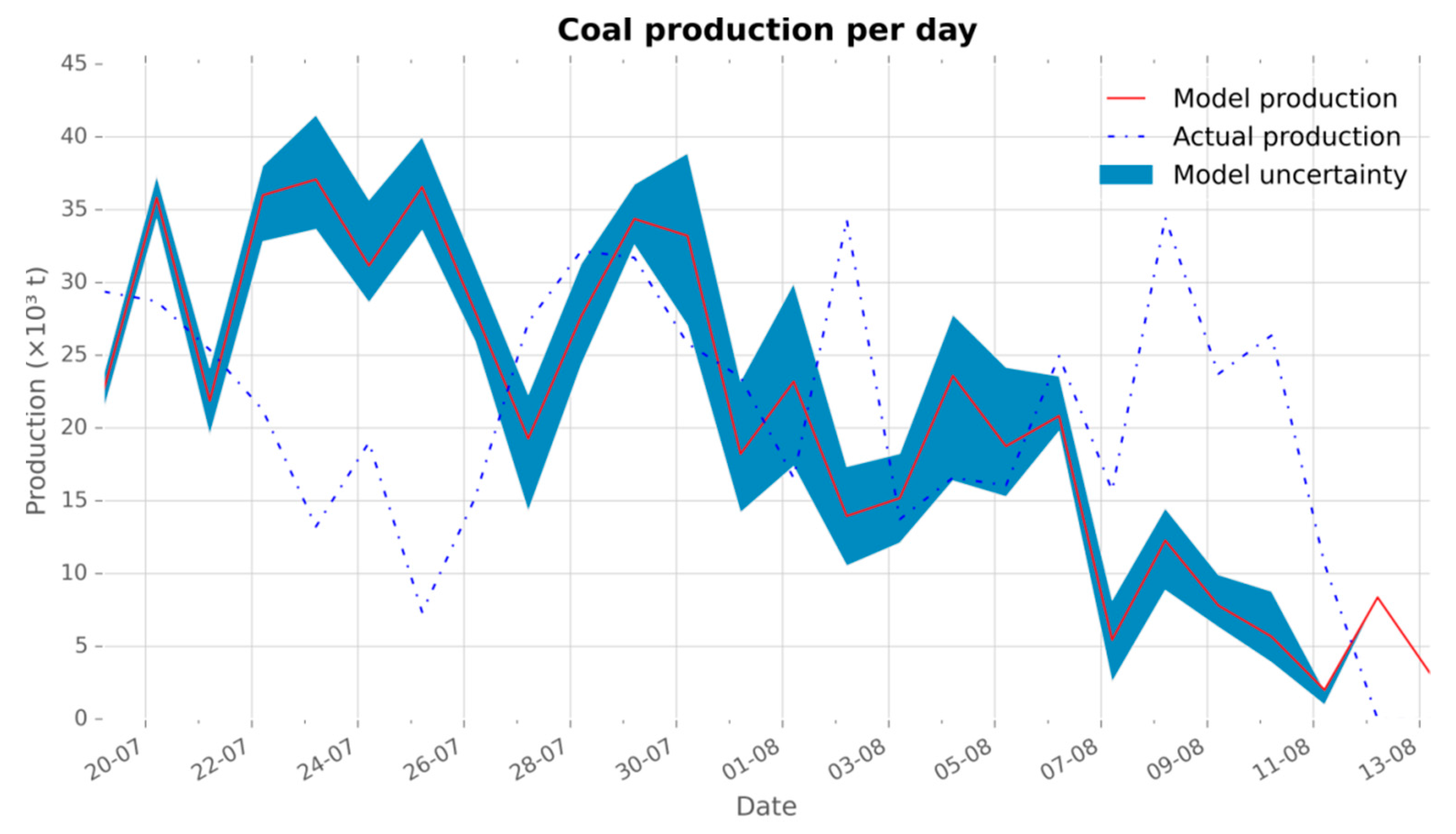
Figure 15.
Comparison of daily production of waste, Experiment 2.
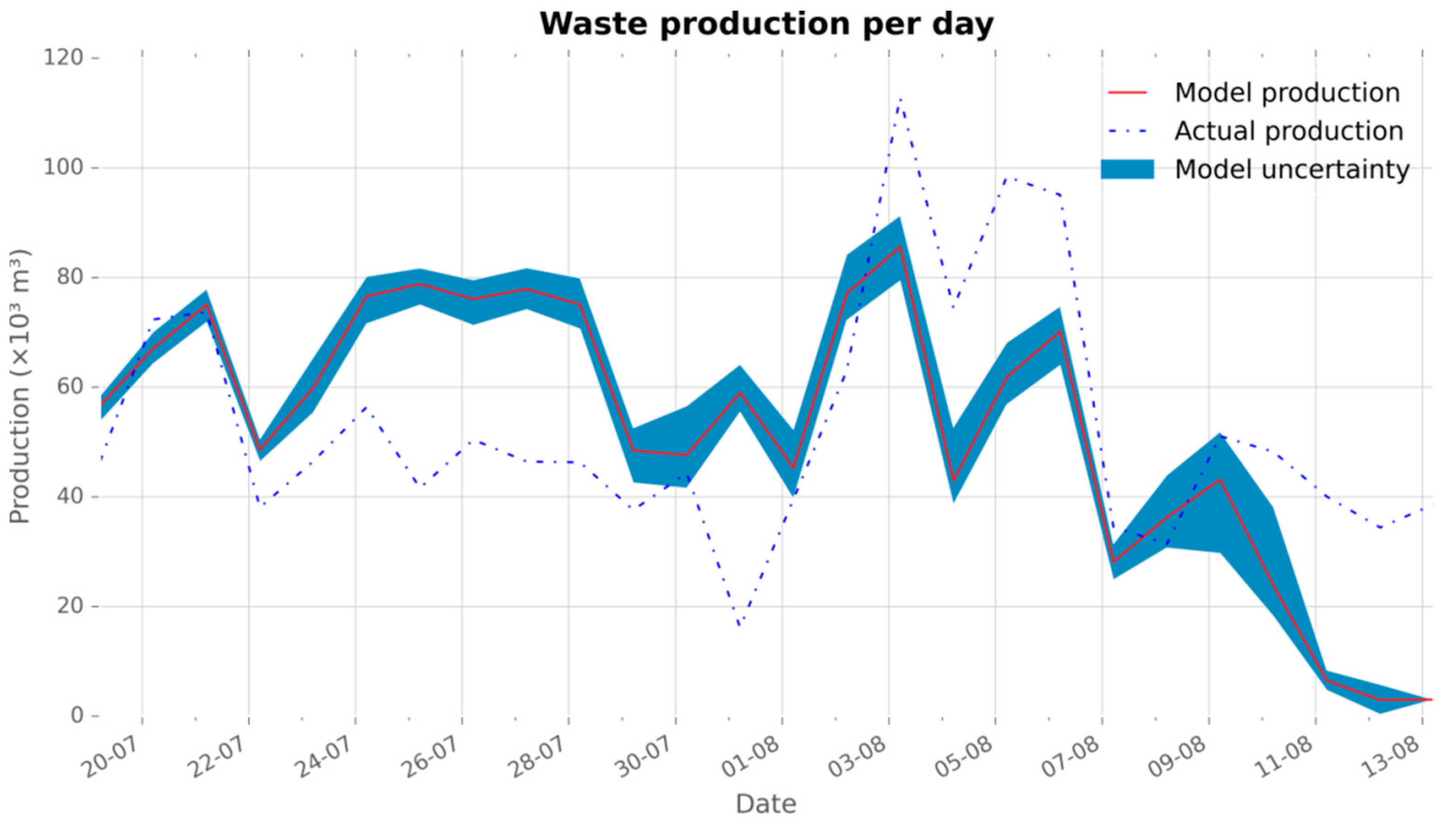
Figure 16.
Daily ash values per day, case Profen.

Figure 17.
Comparison of daily production of coal, Experiment 3.
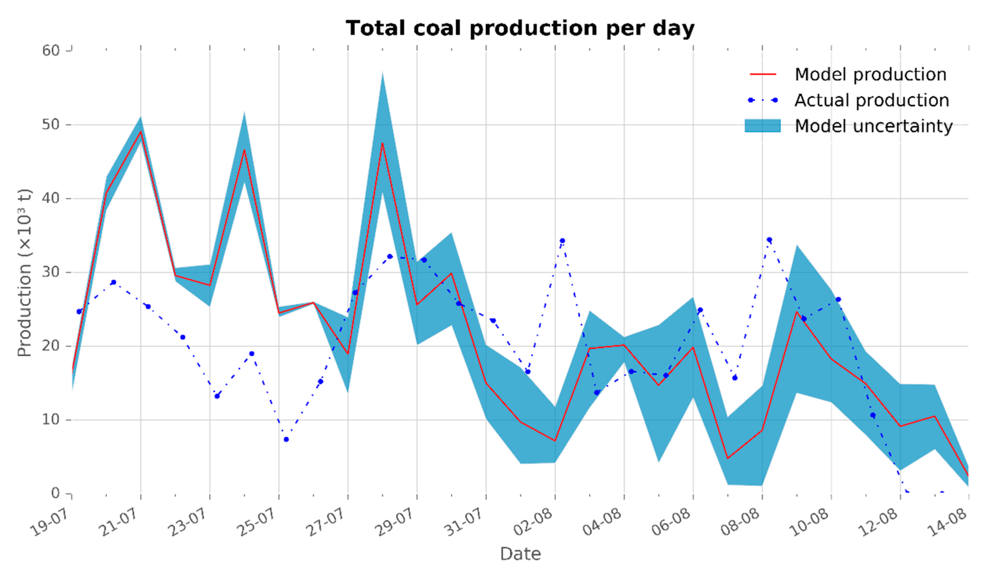
Figure 18.
Comparison of daily production of waste, Experiment 3.

Figure 19.
The total shift-based production of the Hambach mine, Experiment 1.

Figure 20.
The shift-based production of different materials of the Hambach mine, Experiment 1.
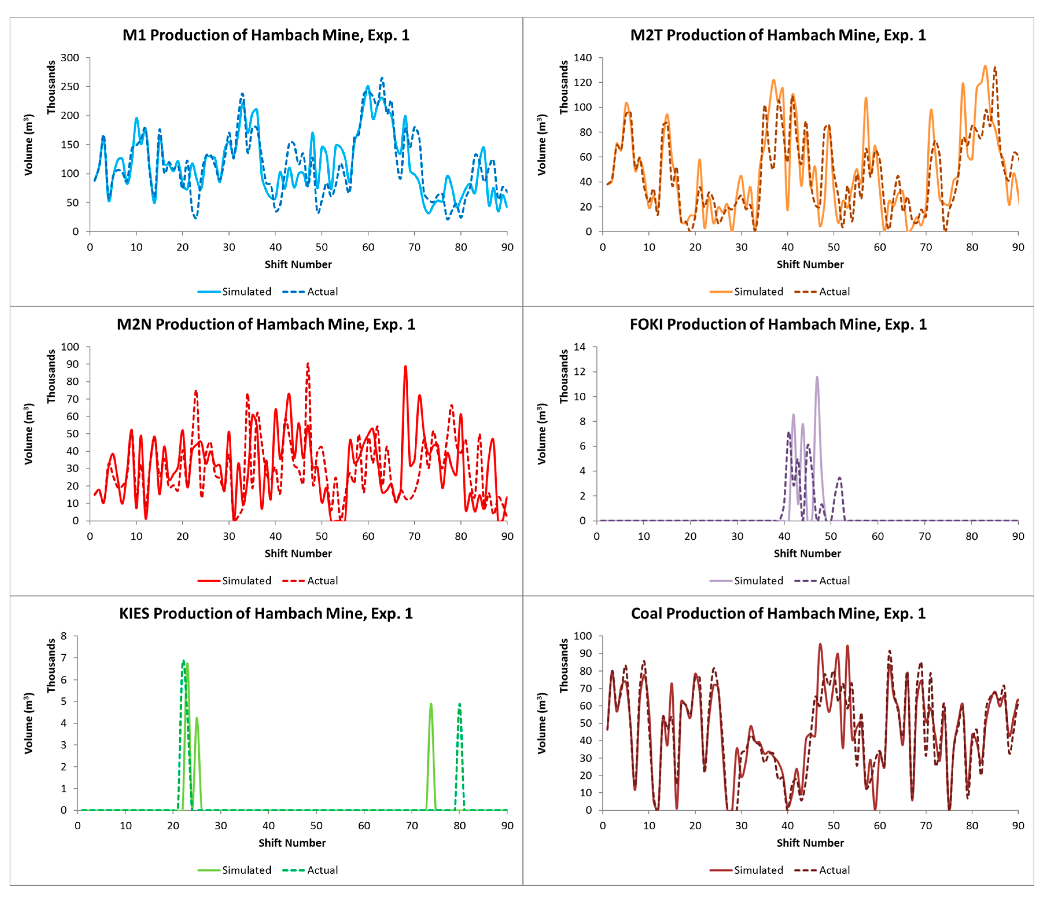
Figure 21.
The total shift-based production of the Hambach mine, Experiment 2.
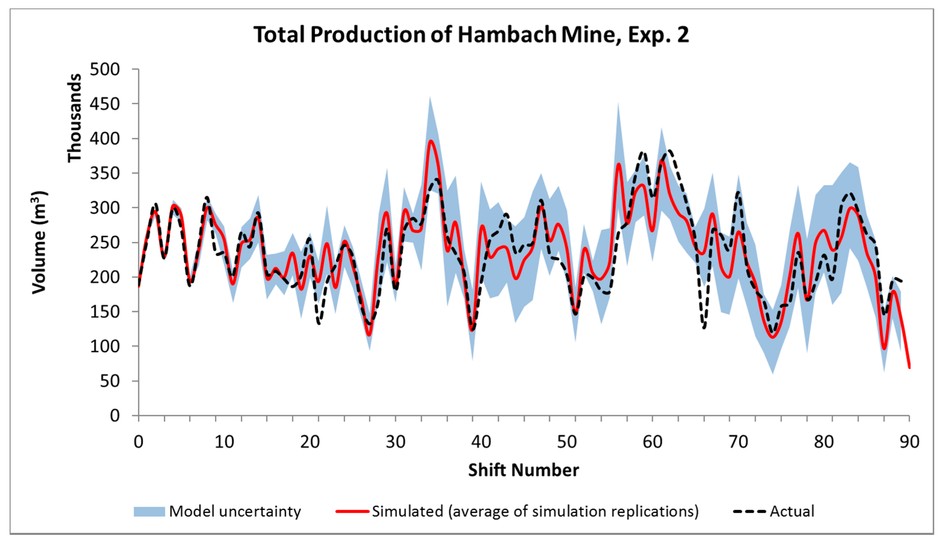
Figure 22.
The shift-based production of different materials of the Hambach mine, Experiment 2.
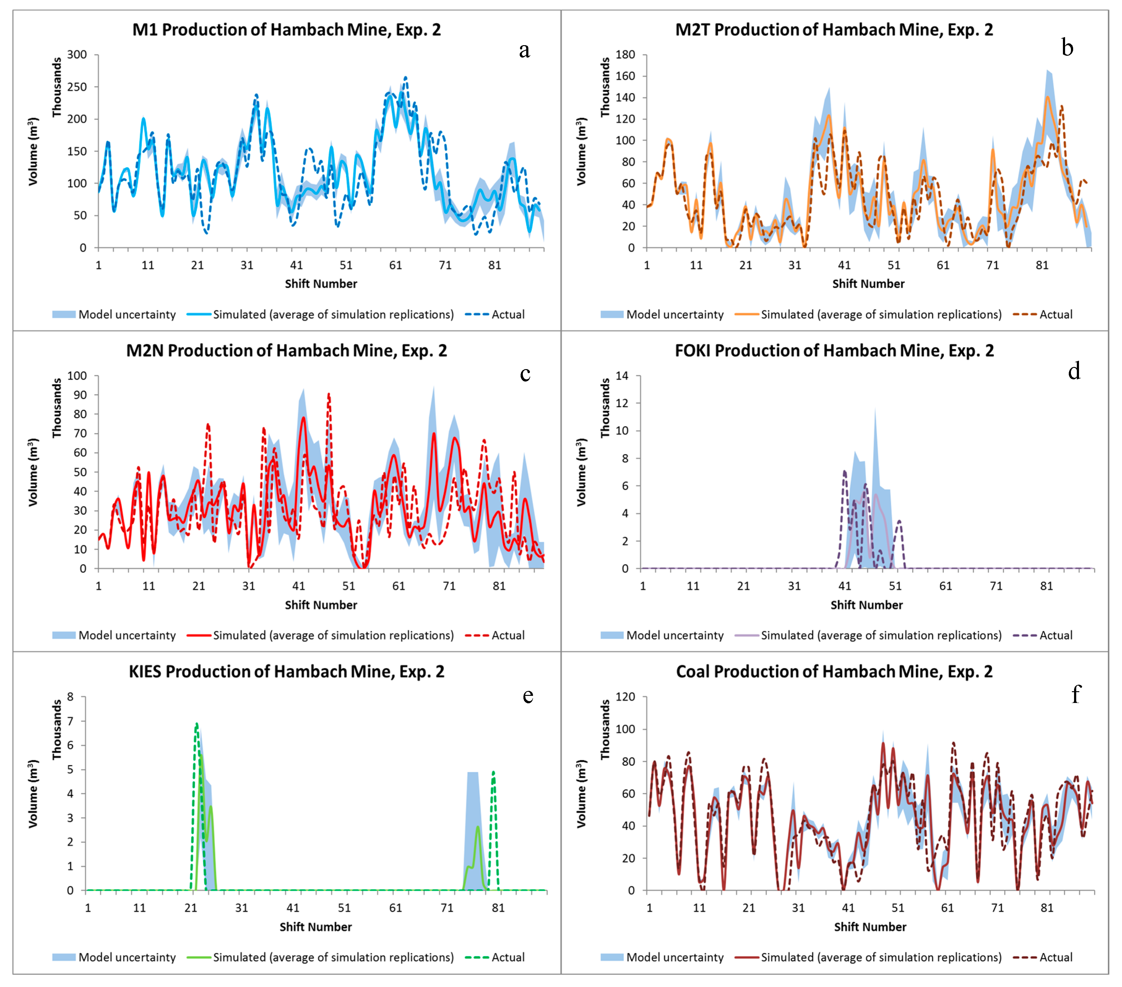
Figure 23.
Utilization of the equipment in the form of pie charts.

Table 1.
Technical specification of BWEs.
| Bench | BWE Model | Discharge Per min | Bucket Capacity (m3) | Theoretical Capacity (m3/h) * |
|---|---|---|---|---|
| S1 | 259 | 44 | 2.6 | 5700 |
| B1 | 260 | 38 | 3.5 | 5700 |
| B2 | 291 | 48 | 5.0 | 12,500 |
| B3 | 287 | 43 | 5.1 | 10,400 |
| B4 | 290 | 48 | 5.0 | 12,500 |
| B5 | 292 | 48.6–72.0 | 5.0 | 12,500 |
| B6 | 293 | 48.6–72.0 | 5.0 | 12,500 |
| B7 | 289 | 48 | 5.0 | 12,500 |
* 19.3 h per day.
Table 2.
An overview of the specifications of the equipment.
| Exc. Model | Bench | Access to Abs. 1112 | Access to Abs. 1104 | Access to Coal-bunker | Theoretical Capacity (m3/h) |
|---|---|---|---|---|---|
| Bg. 1580 | 1 | No | Yes | No | 4900 |
| Bg. 1511 | 2 | Yes | Yes | Yes | 4900 |
| Bg. 1553 | 3 | Yes | Yes | Yes | 3770 |
| Bg. 351 | 4 | Yes | No | Yes | 1400 |
| Bg. 1541 | 5 | Yes | No | Yes | 3770 |
| Bg. 309 | 6 | Yes | No | Yes | 740 |
| Abs. 1112 | - | - | - | - | 10,000 |
| Abs. 1104 | - | - | - | - | 10,000 |
Table 3.
Coal types and their properties.
| Coal Type | Ash Content (%) | Calorific Value (MJ/kg) |
|---|---|---|
| KK1 | <8.5% (wet ash) | 9.5–10.5 |
| KK2 | <12% (wet ash) | 9.0–11.4 |
| SK | <15% (dry ash) | >24.5 |
Table 4.
The required data for building a simulation model.
| Process Related Data |
|
| Elements Related Data (for Each Piece of Equipment) |
|
| Geological Related Data |
|
Table 5.
Summary statistics of simulated and actual production data of the case Profen, Exp. 1.
| Material Type | Simulated | Actual | Difference (%) | Bias (m3 or t) | Average Deviation (m3 or t) | Average Relative Error per Day (%) |
|---|---|---|---|---|---|---|
| Coal (10³ t) * | 533.01 | 533.06 | −0.01 | −0.05 * | 5.02 * | 26.30 |
| Waste (10³ m3) | 1336.28 | 1378.03 | −3.03 | −41.75 | 10.66 | 23.62 |
| Total (10³ m3) | 1794.81 | 1841.56 | −2.54 | −46.74 | 8.49 | 15.25 |
* The unit is tons.
Table 6.
Summary statistics of simulated and actual production data of the case Profen, Exp. 2.
| Material Type | Simulated | Actual | Difference (%) | Bias (m3 or t) | Average Deviation (m3 or t) | Average Relative Error per Day (%) |
|---|---|---|---|---|---|---|
| Coal (10³ t) * | 541.96 | 533.06 | 1.67 | 8.90 * | 10.36 * | 62.55 |
| Waste (10³ m3) | 1373.68 | 1378.03 | −0.32 | −4.34 | 20.19 | 47.22 |
| Total (10³ m3) | 1844.95 | 1841.56 | 0.18 | 3.39 | 24.08 | 40.76 |
* The unit is tons.
Table 7.
Utilization predicted by the simulation model.
| Status | Bg. 1580 | Bg. 1511 | Bg. 1553 | Bg. 351 | Bg. 1541 | Bg. 309 |
|---|---|---|---|---|---|---|
| Busy | 14.3% | 49.8% | 46.1% | 60.5% | 57.8% | 27.6% |
| Failed | 1.0% | 4.7% | 1.7% | 3.7% | 1.1% | 0.6% |
| Idle | - | 7.8% | 37.0% | 3.7% | 8.5% | 7.4% |
| Inactive | 84.7% | 37.7% | 15.3% | 32.3% | 32.5% | 64.5% |
Table 8.
Actual utilization of the system.
| Status | Bg. 1580 | Bg. 1511 | Bg. 1553 | Bg. 351 | Bg. 1541 | Bg. 309 |
|---|---|---|---|---|---|---|
| Busy | 11.7% | 54.0% | 44.7% | 55.8% | 56.7% | 28.2% |
| Failed | 2.9% | 6.9% | 40.9% | 10.9% | 14.8% | 7.1% |
| Inactive | 85.4% | 39.1% | 14.4% | 33.3% | 28.5% | 64.6% |
Table 9.
Differences between the actual and model utilization.
| Status | Bg. 1580 | Bg. 1511 | Bg. 1553 | Bg. 351 | Bg. 1541 | Bg. 309 |
|---|---|---|---|---|---|---|
| Busy | 2.6% | −4.2% | 1.4% | 4.7% | 1.1% | −0.7% |
| Failed | −1.9% | −2.2% | −39.2% | −7.2% | −13.7% | −6.6% |
| Inactive | −0.7% | −1.4% | 0.8% | −1.0% | 4.1% | −0.2% |
Table 10.
Summary statistics of simulated and actual production data of the case Profen, Exp. 3.
| Material Type | Simulated | Actual | Difference (%) | Bias (m3 or t) | Average Deviation (m3 or t) | Average Relative Error per Day (%) |
|---|---|---|---|---|---|---|
| Coal (10³ t) * | 582.51 | 533.06 | 10.24 | 49.45 * | 12.31 * | 65.90 |
| Waste (10³ m3) | 1402.73 | 1378.03 | 1.54 | 24.7 | 16.33 | 29.29 |
| Total (10³ m3) | 1909.26 | 1841.56 | 3.49 | 67.7 | 18.82 | 24.65 |
* The unit is tons.
Table 11.
Summary statistics of the simulated and the actual production data of the Hambach case, Exp. 1.
Table 11.
Summary statistics of the simulated and the actual production data of the Hambach case, Exp. 1.
| Material Type 1 | Simulated | Actual | Difference (%) | Bias (m3 or t) | Average Deviation per Shift (m3 or t) | Average Relative Error Per Shift (%) |
|---|---|---|---|---|---|---|
| M1 (m³) | 10,604,266 | 10,655,819 | −0.48 | −51,553 | 26,178 | 0.25 |
| M2T (m³) | 4,263,052 | 4,290,314 | −0.64 | −27,262 | 16,965 | 0.40 |
| M2N (m³) | 2,765,828 | 2,765,928 | 0.00 | −100 | 15,050 | 0.54 |
| FOKI (m³) | 33,329 | 33,329 | 0.00 | 0 | 593 | 1.78 |
| KIES (m³) | 16,000 | 16,000 | 0.00 | 0 | 251 | 1.57 |
| Coal (t) | 4,157,393 | 4,183,493 | −0.62 | −26,100 | 7872 | 0.19 |
| Total volume (m³) | 21,297,599 | 21,399,210 | −0.47 | −101,611 | 27,064 | 0.13 |
1 M1, M2T, M2N, FOKI, and KIES are abbreviations for different types of waste materials.
Table 12.
Summary statistics of the simulated and the actual production data of the Hambach case, Exp. 2.
Table 12.
Summary statistics of the simulated and the actual production data of the Hambach case, Exp. 2.
| Material Type | Simulated | Actual | Difference (%) | Bias (m3 or t) | Average Deviation per Shift (m3 or t) | Average Relative Error per Shift (%) |
|---|---|---|---|---|---|---|
| M1 (m³) | 10,556,753 | 10,655,819 | −0.93 | −99,066 | 27,892 | 0.26 |
| M2T (m³) | 4,257,161 | 4,290,314 | −0.77 | −33,153 | 14,912 | 0.35 |
| M2N (m³) | 4,257,161 | 4,290,314 | −0.77 | −33,153 | 14,610 | 0.34 |
| FOKI (m³) | 33,329 | 33,329 | 0.00 | 0 | 414 | 1.24 |
| KIES (m³) | 16,000 | 16,000 | 0.00 | 0 | 251 | 1.57 |
| Coal (t) | 4,060,603 | 4,183,493 | −2.94 | −122,890 | 9336 | 0.22 |
| Total volume (m³) | 23,181,006 | 23,469,269 | −1.23 | −288,263 | 30,938 | 0.13 |
© 2017 by the authors. Licensee MDPI, Basel, Switzerland. This article is an open access article distributed under the terms and conditions of the Creative Commons Attribution (CC BY) license (http://creativecommons.org/licenses/by/4.0/).
Share and Cite
MDPI and ACS Style
Shishvan, M.S.; Benndorf, J. Operational Decision Support for Material Management in Continuous Mining Systems: From Simulation Concept to Practical Full-Scale Implementations. Minerals 2017, 7, 116. https://doi.org/10.3390/min7070116
AMA Style
Shishvan MS, Benndorf J. Operational Decision Support for Material Management in Continuous Mining Systems: From Simulation Concept to Practical Full-Scale Implementations. Minerals. 2017; 7(7):116. https://doi.org/10.3390/min7070116
Chicago/Turabian StyleShishvan, Masoud Soleymani, and Jörg Benndorf. 2017. "Operational Decision Support for Material Management in Continuous Mining Systems: From Simulation Concept to Practical Full-Scale Implementations" Minerals 7, no. 7: 116. https://doi.org/10.3390/min7070116
Note that from the first issue of 2016, this journal uses article numbers instead of page numbers. See further details here.