Article

Signal Estimation Using Wavelet Analysis of Solution Monitoring Data for Nuclear Safeguards

Statistical Sciences, Los Alamos National Laboratory, Los Alamos, NM 87545, USA
*
Author to whom correspondence should be addressed.
Axioms 2013, 2(1), 44-57; https://doi.org/10.3390/axioms2010044
Submission received: 31 January 2013 / Revised: 4 March 2013 / Accepted: 7 March 2013 / Published: 20 March 2013
(This article belongs to the Special Issue Wavelets and Applications)

Abstract

:
Wavelets are explored as a data smoothing (or de-noising) option for solution monitoring data in nuclear safeguards. In wavelet-smoothed data, the Gibbs phenomenon can obscure important data features that may be of interest. This paper compares wavelet smoothing to piecewise linear smoothing and local kernel smoothing, and illustrates that the Haar wavelet basis is effective for reducing the Gibbs phenomenon.

1. Introduction

Wavelets are an effective tool for many applications, including change detection and data smoothing. This paper’s focus is on data smoothing. One challenge for any smoothing method is the bias associated with rapid signal change regions [1]. A specific example of bias in wavelet smoothing is the Gibbs phenomenon, which appears in the reconstructed signal as large oscillations that can obscure important data features.
Wavelet analysis applied to solution monitoring (SM) data in nuclear safeguards provides a unique reason to mitigate the Gibbs phenomenon. Methods for minimizing the Gibbs phenomenon will be presented and illustrated on simulated SM data. The Gibbs phenomenon has been detected in continuous wavelet transformations of continuous data at jump discontinuities in the signal [2]. A definition of the Gibbs phenomenon for wavelets analysis is given in Section 4. More generally, all smoothers have difficulty fitting functions in regions of rapid signal change [1].
Wavelets are an attractive smoothing option because of their ability to model different patterns in the data. In previous research, piecewise linear regression (PLR) was shown to be the best method among those evaluated (which included one type of wavelet smoothing) for smoothing SM data, where “optimal” was defined as the method that minimizes the root mean squared error (RMSE) [3]. However, Burr et al. [3] did not attempt to tune wavelets to make them have as small a RMSE as possible for the analysis of SM data. This paper describes our effort to tune wavelet smoothing to its optimal performance on SM data. Tuned wavelet smoothing is then compared to PLR smoothing and to local kernel smoothing.
The following section describes the SM application. Section 3 describes our simulated data. Section 4 gives results.

2. Solution Monitoring for Nuclear Safeguards
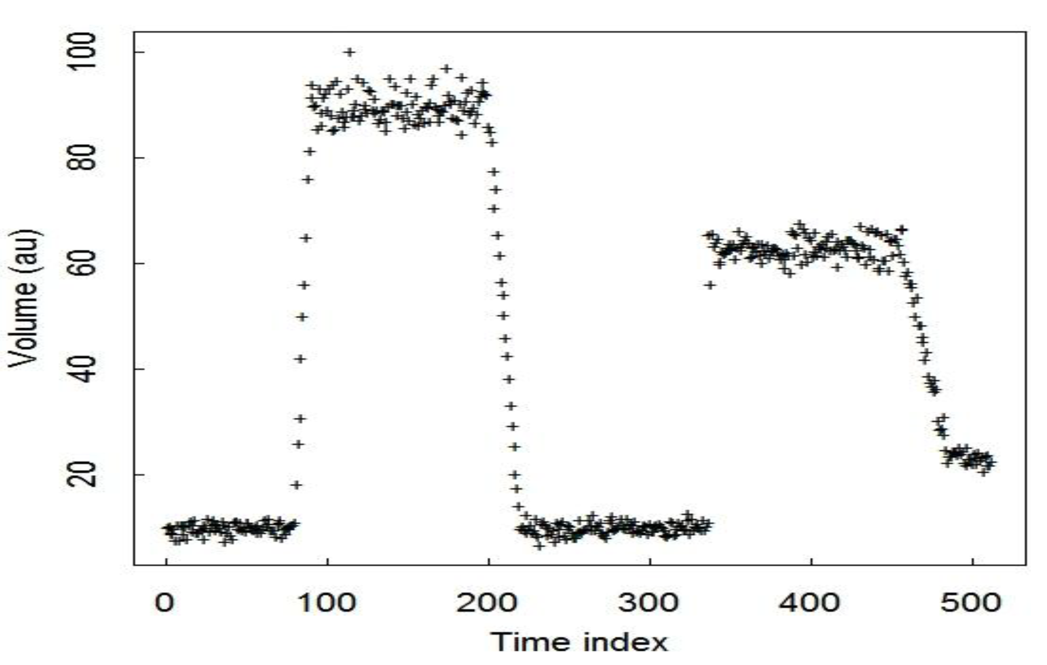
This paper’s wavelet application is SM at large commercial aqueous reprocessing plants. It is well understood that because nuclear material accountancy (NMA) measurement uncertainty increases as facility throughput increases, in spite of sustained efforts to reduce measurement uncertainty, it remains difficult to satisfy the International Atomic Energy Agency diversion detection goal for large throughput facilities [4].
NMA at a declared and safeguarded facility involves measuring facility inputs, outputs, and inventory to compute a material balance defined as MB = T in + I begin - T out - I end , where T is a transfer and I is an inventory. The main quantitative assessment of safeguards effectiveness is the measurement error standard deviation of the material balance.
Partly in response to shortcomings of NMA alone, process monitoring (PM) is used as an additional measure to bolster NMA [4]. While it is generally agreed that PM adds value to safeguards, its possible roles and benefits are not fully understood. The main goal for using PM in addition to NMA is to improve the ability to detect off-normal plant operation.
As an example of PM, SM is a type of PM in which masses and volumes are estimated from frequent in-process measurements [5,6,7,8]. If each tank is regarded as a sub-MBA (material balance area), then transfers between tanks can be identified, segments of which can then be compared to generate transfer differences (TDs). A safeguards concern might then be raised if either these TDs or deviations in mass or volume data during “wait” modes become significant [3,6,8]. Average mass and volume TDs should be zero (perhaps following a bias adjustment) to within a historical limit that is a multiple of the standard deviation of the TD, as should deviations during “wait” modes. A residual (residual = measured − predicted) is generated each time a mode (transfer or wait) is completed by any tank. Such residuals can be analyzed over time and over tanks. Analogously, in NMA one can analyze MBs for time trends.
Measurement error effects in real SM data suggest that the standard deviation of the mass or volume TD in tank-to-tank transfers is approximately 5 to 10 times larger than international target values [9] and tank calibration studies suggest [5,6,7]. Reasons for the larger-than-anticipated standard deviation in the TDs include failure to adequately smooth the mass and volume data (this paper’s focus), imperfect event marking, and process variation effects such as varying evaporation rates, varying amounts of solution carryover due to pipes and pump behavior, and temperature changes that impact volume measurements [10].
It is not anticipated that safeguards personnel will routinely evaluate the large amounts of data generated from monitoring all transfers and wait modes for all tanks. Instead, some type of monitoring system will flag only anomalous transfers and wait modes [3]. In-tank dip tubes located at various tank heights measure pressures that can be converted to density and to volume via a level-to-volume calibration. Solution mass in the tank is then calculated as volume times density. For our purposes here, it is sufficient to consider only discrete time series of tank volume. Analysis, for example, of tank mass is similar.
Figure 1 is realistic simulated measured volumes which are denoted throughout as M(t) or Mt. These simulated volumes are in arbitrary units (au), include measurement error, and illustrate the challenges to be considered here, including changes in shipping and/or receiving rates and different spacings between events such as tanks filling and emptying. Tank transfer mode involves a shipper and receiver tank. Tank wait mode involves only one tank, but could involve transient behavior such as recirculation or evaporation.
Figure 1. Simulated volume measurements Mt in arbitrary units (au) at each of 512 time indices.
Axioms 02 00044 g001
Measured readings Mt (which will be regarded as volume in this paper) will have measurement errors present, and generally there could be both relative and absolute errors. Tank data arrives in a streaming fashion, approximately every 30 s or even more frequently. This work focuses on material monitoring, not on material control, so extremely timely decisions regarding whether there are any abnormal plant operations are not necessary and so are not considered here. Instead, in this application, we can retrospectively analyze sections of approximately the most recent one day’s worth of data to detect abnormal plant operations. The main implication of this is that at any time step to be evaluated, one can retrospectively look both forward and backward in modest time intervals contained entirely within the one-day analysis window. In contrast, [11], for example, described a scheme to filter tank data online, removing Mt if Mt is similar in value to Mt−1, removing outliers, and removing Mts associated with sparging events. Here, it is also desired to remove outliers and Mts associated with sparging events, leaving only marked “wait modes” and marked “transfer modes” to evaluate in each tank.
One goal here is to quantify the RMSE in estimated tank receipts and shipments that arises due to the combination of imperfect event marking and the measurement error standard deviations that characterize how well the pre and post transfer levels are measured. Any remaining RMSE in real data is assumed to arise from the temporary give and take associated with solution transfer mechanisms [10].

3. Simulated Data

In NMA, SM data includes time series of volumes from tanks at a nuclear facility. This data is recorded at discrete time steps, typically every few minutes, and can be modeled by
M ( t ) = T ( t ) + T ( t ) ϵ R + ϵ A
where M ( t ) is the measurement at time t, and T ( t ) is the true value which is assumed to be unknown. Additive and relative errors are assumed to be Gaussian distributed as
ϵ R ~ N ( 0 ,   σ R )  and  ϵ A ~ N ( 0 ,   σ A )
One advantage of using simulated data is that the true values are known, so the RMSE of data smoothers can be estimated accurately. Many simulated datasets (see Section 5) were created in the R statistical programming language [12] to represent real SM data, and each data set included random relative and additive errors generated from independent normal distributions using Equations (1) and (2). Typical values for σ R range are from approximately 0.001 (0.1%) to 0.03. Typical values for σ A depend on the measurement units and for the range of T values we consider, σ A ranges from approximately 0.1 to 2 [5,6]. This paper uses nominal values of σ A = 0.5 or 1 and σ R = 0.015 for additive and relative errors, respectively.
Many types of events are observed in real data and corresponding simulated data were created to include events that frequently occur [3]. The model defined by Equations (1) and (2) is adequate for assessing the performance of smoothing methods for SM data.

4. Wavelets

Wavelets can estimate an unknown function such as T ( t ) by expanding a known (observed) function, such as M(t) as defined in (1), into a wavelet series [13,14,15,16,17,18,19,20,21,22,23]. Discrete or continous transformations can be used on SM data. In this paper, discrete transformations are used. The process of wavelet smoothing using a discrete wavelet transform is outlined below.
1)
M(t) is decomposed using a discrete wavelet transformation;
j ϵ k ϵ w j k ψ j k ( t )
where
w j k = M ( t ) ψ j k ( t ) d t
are wavelet coefficients. Note that these coefficients are obtained from noisy data and are therefore also disturbed by noise with
w j k = w j k * + ε
such that ε is error and w j k * are the true coefficients.
2)
Using a wavelet thresholding method, an estimate of the true noiseless coefficients is found. These are denoted w ^ j k . Wavelet thresholding sets w j k below a certain threshold to 0.
3)
The data is reconstructed using an inverse discrete wavelet transform with w ^ j k to obtain and estimate of the noiseless data
T ^ ( t )= jϵZ kϵZ w ^ jk ψ jk (t)T(t)
One requirement when using wavelets to approximate data is that the data must be of a dyadic length ( 2 j     for     j ). SM data is plentiful so it is easy to break the data into dyadic sections. All simulated datasets have dyadic length (usually 256, 512, or 1024) to keep the analysis as simple as possible. Wavelet smoothing is easily implemented in R using any of several wavelet packages, such as wavethresh, which we use here.

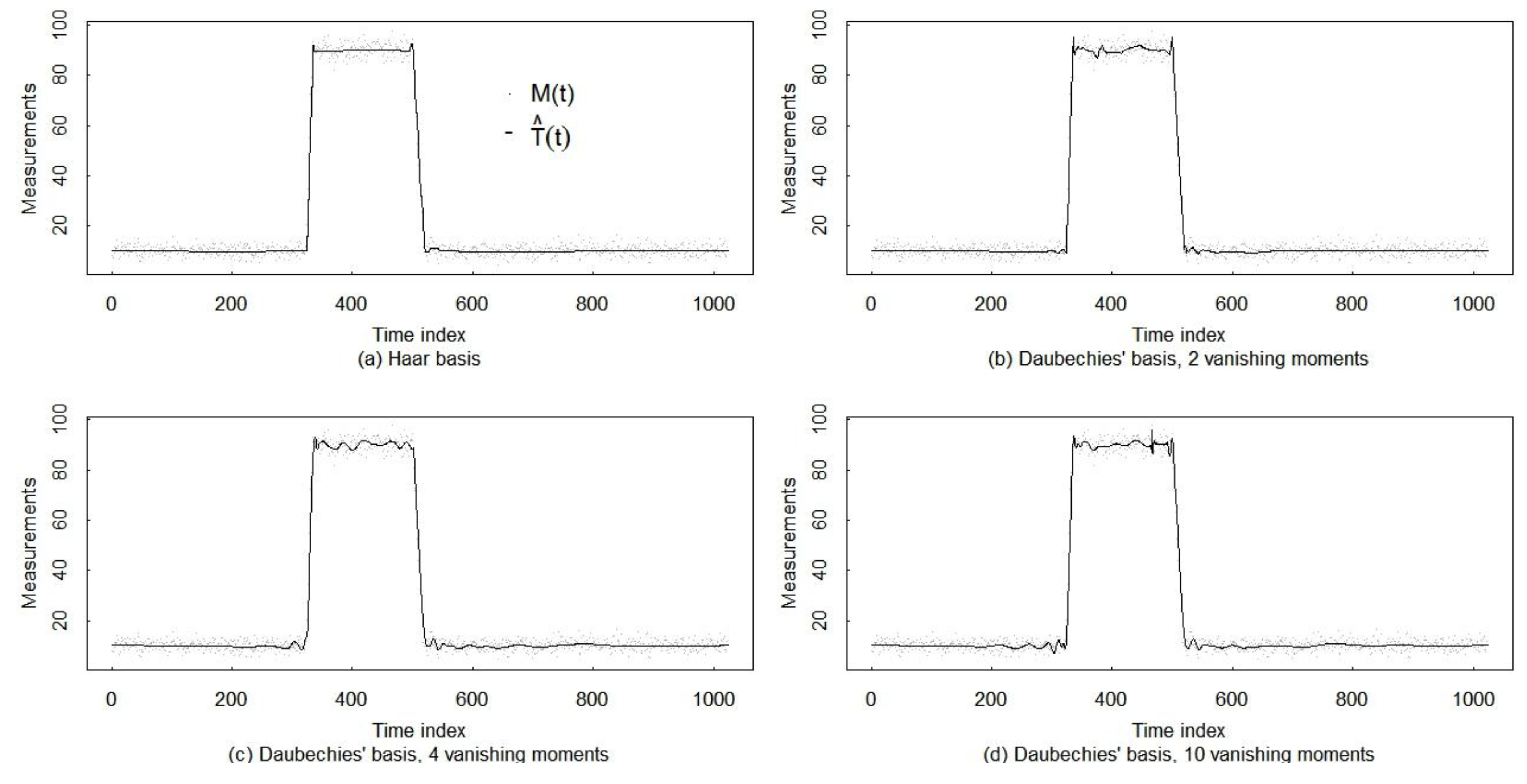
4.1. The Gibbs Phenomenon in Wavelet Analysis

In Fourier analysis, the Gibbs phenomenon is the tendency of a reconstructed signal to underestimate or overestimate the true value at jump discontinuities, causing oscillations in the reconstructed signal [24]. This oscillation has also been observed in wavelet analysis [2,24,25]. The phenomenon affects both smoothing and change detection because it obstructs the change points (change detection application), and adds to an overall poor fit to the data (smoothing application). The Gibbs phenomenon is known to arise as a result of using a continuous wavelet function base to approximate discontinuous (or discrete) data [24]. The wavelet approximation of a signal tends to oscillate near large change points in data sampled at discrete time, and these oscillations do not diminish as the number of wavelet functions used in the approximation increases.
More generally, in data that does not have discontinuities, but has rapid changes in slope, such as SM data, all smoothers are known to have bias near regions of rapid signal change [1,3].

4.2. Mathematical Description of the Gibbs Phenomenon

In the context of SM data, M(t) is a discrete time series such that M ( t ) : [ 0 ,   n ] , where t, M 0 . Let N + . Assume t 0 is a change point, defined as a point where the time dependence of T(t) changes [22]. More specifically, in SM we assume that T(t) is piecewise linear with unknown breakpoints where the slope changes. Let t N be a sequence convergent to t 0 as N → ∞. For each N > 1, let T ^ N ( t ) be the Nth partial wavelet series
T ^ N ( t ) = j ,   k N w ^ j k · ψ j k ( t )
Then
| lim N T ^ N ( t 0 ) | > T ( t 0 )
Therefore,   T ^ N ( t 0 ) does not converge to T ( t 0 ) as N → ∞, so the oscillations due to the Gibbs phenomenon do not diminish as N → ∞. The Gibbs phenomenon is not restricted to the discrete case. The mathematical description of Gibbs phenomenon in continuous wavelet analysis follows analogously. In the continuous case the wavelet approximation to the data is represented by
T ^ N ( t ) = 0 N w ^ j k · ψ j k ( t ) d t
The Gibbs phenomenon has been observed at jump discontinuities in wavelet smoothing [2], and is observed in discrete SM data. There are no jump discontinuities in this SM data because it is from a physical process that is everywhere continuous. However, there can be abrupt changes made over one or more time steps where the slope changes and so the true value T(t) is not everywhere differentiable. The Gibbs effect appears at abrupt change points, which obscures these change points and interferes with proper event detection and data smoothing.

4.3. Example of the Gibbs Phenomenon

In graphical and RMSE comparisons of wavelet smoothing using different wavelet families, we have found and show in Section 5 that the Gibbs effect tends to be minimized by using Haar wavelets [25]. Simulated shipment and receipt examples (such as in Figure 1) were purposely chosen to include abrupt events to illustrate severe cases of Gibbs phenomenon in both graphical and RMSE comparisons.
In Figure 2, the wavelet families used are Haar wavelets, Daubechies’ wavelets with 2 and 4 and 10 vanishing moments, as labeled in the figure. The four wavelets families in Figure 2 are described in [13]. A Bayesian thresholding method was used to retain only the most significant wavelet coefficients [23] for data smoothing. Note that the Gibbs phenomenon is smallest in the top left plot, which uses the Haar wavelet basis.
Figure 2. Comparison of the Gibbs phenomenon for various wavelets.
Axioms 02 00044 g002

4.4. Mitigation of the Gibbs Phenomenon

The Gibbs effect exists for all wavelet series approximations (except for Haar wavelets in continuous data or if special types of summations are used [25]), but one way to reduce the Gibbs effect is to use the Haar wavelet family when decomposing the function [2,25]. A property of the Haar wavelet basis is that if the change point is centered in the dataset, the Gibbs effect does not appear in the reconstructed data [26]. For SM data, the locations of the change points are unknown, so this method cannot easily be implemented. However, the Haar wavelet family can still greatly reduce the Gibbs effect in SM data, as seen in Figure 2. For this reason, Haar wavelets are used throughout this paper. Other wavelet families may be optimal for different types of data.

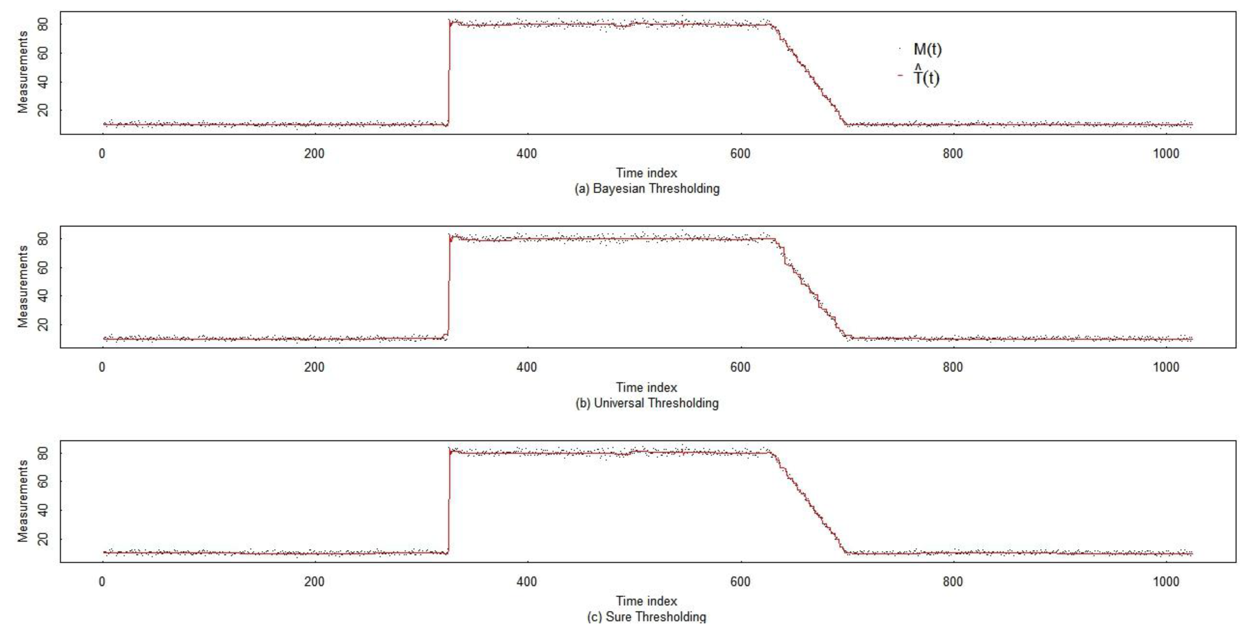
5. Simulation Results

5.1. Wavelet Smoothing

There are many methods for thresholding wavelet coefficients in order to smooth noisy data. This section compares three thresholding methods: Bayesian [19], Universal [15], and SURE [14]. The quality of the fit T ^ i of the smoothed data to the signal T i can be measured across all n time indices by the RMSE or by the relative RMSE (RRMSE), calculated, respectively, as
RMSE = 1 n i = 1 n ( T ^ i T i ) 2   and   RRMSE = 1 n i = 1 n ( T ^ i T i ) 2 T i 2
Because in our simulated SM data the true value T i is known, the RMSE and RRMSE can easily be calculated. In previous SM analysis, data was simulated having a modest range of event types [3], some of which had the Gibbs phenomenon present. In [3], soft Bayesian thresholding with Daubechies’ wavelets using 10 vanishing moments was used without comparison of other wavelet bases or other thresholding options to mitigate the Gibbs phenomenon. Here, data of dyadic length n was decomposed, thresholded, and reconstructed to obtain T ^ ( t ) . All thresholding and methods and wavelet bases choices were easily implemented in R using the package wavethresh [20].
The RMSE and RRMSE results were very similar using either hard or soft thresholding. Also, whether to transform the data to approximately unit variance by first performing an initial smoothing made very little difference. The reason we evaluated whether transforming to approximately unit variance is as follows. To the best of our knowledge, wavelet literature assumes purely additive error models [16] rather than the combination of additive and multiplicative errors in Equation (1) that are more appropriate for SM data [5]. If the true value T t at each time step t were known exactly, then rescaling M(t) by dividing by σ A 2 + T t 2 σ R 2 would convert the time series to a unit variance time series with purely additive error. Because T t is unknown, it must be estimated using T ^ t , which we obtained using an initial Harr-based wavelet transform. Because of estimation error in T ^ t , the scaled M(t) has only approximately unit variance, and departures from unity tend to occur near the change points.
The estimated RMSE of many trials is assumed to be normally distributed across sets of simulations, and the average over 10 sets of 30 trials is reported in Table 1. Table 1 shows the RMSE results for simulated data including an abrupt event and a gradual event as shown in Figure 3. Entries are repeatable within approximately ± 2 σ ^ 10 , where σ ^ is the estimated standard deviation across sets of 30 trials.
Figure 3. Smoothing base on bayesian, universal, and sure thresholding on simulated data. Bayesian thresholding appears to be the best method of de-noising this data.
Axioms 02 00044 g003
Table 1. The RMSEs for data including 1 abrupt and 1 gradual event over 1024 data points as in Figure 3.
Bayesian softUniversal softSure soft
0.6822 ±0.0080.8975 ±0.0050.8079 ±0.007

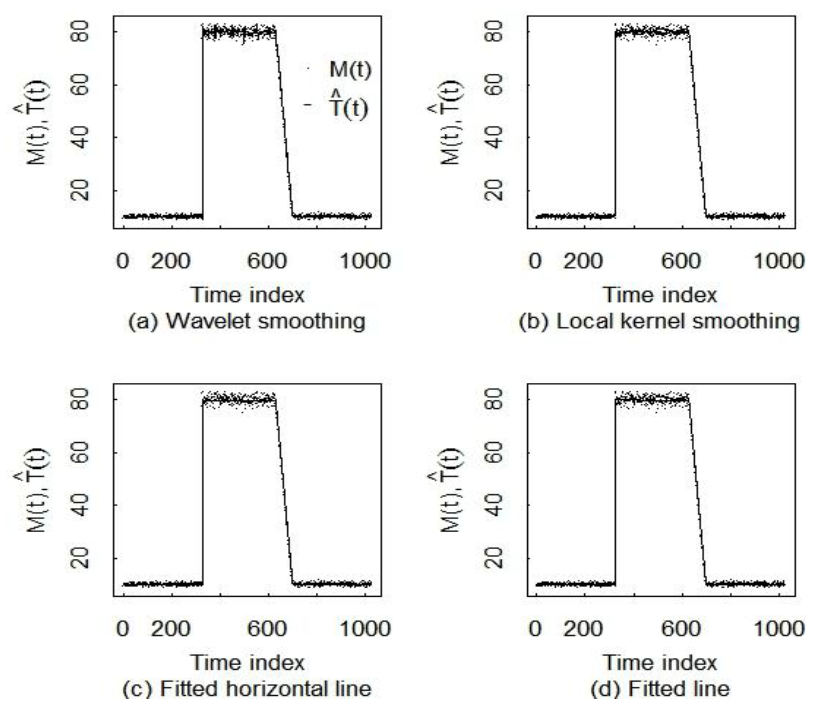
5.2. Comparison of Three Smoothing Methods

Smoothing techniques that have been used on SM data include piecewise linear regression (PLR), local kernel smoothing using lokerns in R, and wavelet smoothing with no attempt to optimize the wavelet smoothing (see Section 5.1) for SM data [3]. In this section all three methods are compared and several wavelet smoothing options are considered. Simulated data includes a rapid receipt occurring over one time step and a gradual shipment and also a gradual receipt and gradual shipment, all with additive and relative noise as in Figure 1. This simulated SM data has a true value T(t) that is exactly piecewise linear, so PLR is expected have the lowest RMSE. However, using PLR in practice introduces the challenge of estimating the location of the change points so that the data can be adequately broken into pieces.
First, for comparing kernel regression and Harr-wavelet smoothing to the best possible version of PLR, we assumed change points were known, and PLR was used to smooth the data. There are two cases for PLR in SM. In one case the regions are known to be flat, in the other case the regions are not known to be flat. One reason for allowing for the possibility of non-flat T(t) even in “wait” modes is solution evaporation. In general we cannot know whether to assume flat or non-flat T(t), so among the RMSE results reported, those that assume non-flat T(t), which leads to slightly larger RMSE than if we could correctly assume flat T(t), are the most relevant to the SM application.
The RMSE was calculated in time windows that include the change points and in the “wait” regions where change points do not occur. These four smoothing methods are shown in Figure 4. As expected, the RMSE is largest near change points. The average of 10 sets of 30 trials is reported in Table 2, where entries are repeatable to approximately ± 2 σ ^ 10 .
Figure 4. Four smoothing methods on simulated data.
Axioms 02 00044 g004
Table 2. The RMSE of smoothed data. PLR is piecewise linear regression and lokerns is local kernel smoothing. Notice that wavelet smoothing does better than lokerns near the change points. The “any line” option of PLR is the most relevant for SM data.
Haar waveletslokernsPLR (flat line)PLR (any line)
data length 2100.46 ± 0.0050.71 ± 0.0020.057 ± 0.0020.075 ± 0.002
near change points0.91 ± 0.0153.60 ± 0.0150.118 ± 0.0060.141 ± 0.006
away from change points0.44 ± 0.0030.31 ± 0.0020.054 ± 0.0030.069 ± 0.002
Recall that up to this point we assumed that the change points were known exactly for PLR. In practice, the change point locations must be estimated. To estimate change point locations, we have found that approaches such as the approach available in the breakpoints function in R do not work well unless the true number of break points is known in each data region analyzed. The breakpoints function uses dynamic programming to increase the speed of searching for the best number and location of change points, with PLR applied between each change point. However, the breakpoints function is very slow (several minutes on a modern desktop) to run inside each simulation loop. In addition, we have found breakpoints to provide very unstable estimates of the number of change points [23].Therefore, as described in [23], we first use wavelets for initial change-point detection, then refine the initial estimate of each break point location using a “find-one-changepoint-at-a-time” version of the breakpoint function (see the Notes Section [27]).
Example RRMSE values for this strategy, which includes the effect of estimation error in the change points are given in Table 3 for the four wavelet smoothers shown in Figure 2, for lokerns, and for two versions of PLR. In one version of PLR, the fitted line is used to predict T(t) in each region. In the other version of PLR, the fitted line is used to predict T(t) over “wait” regions, but is not used in “transfer” regions. Instead, in the transfer regions, the unsmoothed M(t) values are used to predict T(t). Each entry is repeatable to within approximately ± 0.003 or smaller. The 1000 sets of simulated data used to calculate the RRMSE values in Table 4 all included a modest receipt rate and modest ship rate, each occurring over 10 time steps. And, the 1000 sets of simulated data had an additional noise source which we call “synchronization error”. Because the times of flow rate changes that occur during transfers could be out of time step with the data collection times, the first time step in each transfer could have a slightly different rate of change than the other time steps. This was simulated by allowing for a uniform offset with a range from 0 to 0.3 of the time step to mimic having approximately moderate synchronization error in the first (and/or last) time step.
Table 3. The relative RMSE (RRMSE) results for the four wavelet options in Figure 2, and for lokerns and PLR with estimated change points in 1000 simulations. Each RRMSE entry is repeatable to within approximately ± 0.001 or smaller. In PLR1, the fitted line is used to predict T(t) over each region. In PLR2, the fitted line is used to predict T(t) over “wait” regions, but is not used in “transfer” regions. The values σ A = 0.5 and σ R = 0.015 were used for all 1000 simulations.
Wave1Wave2Wave3Wave4lokernsPLR1PLR2
All points0.0070.0120.0170.0170.0180.0030.004
Near change points0.0230.0210.0450.0400.0560.0100.020
Away from change points0.0060.0060.0160.0160.0160.0020.002
Note from Table 3 that wavelet 1 (the Haar wavelet in Figure 2) has the smallest RRMSE among the four wavelet options, and that its RRMSE is remarkably close to the smallest possible RRMSE using PLR with estimated change points. An advantage of the Haar wavelet is that it mitigates the Gibbs effect, and change point estimation is not required as it is with PLR. Recall that Haar wavelets were used to find the initial estimates of the change points, then refined as shown in [27]. Therefore, wavelets play a key role even in PLR. Also note that the RRMSEs for PLR2 are somewhat higher than for PLR1. However, recall that the simulated data had a modest receipt rate and modest ship rate, each occurring over 10 time steps. For more abrupt transfer rates, we have found that using M(t) rather than the PLR-smoothed version of M(t) performs better during transfers. For example, in Table 4 the RRMSEs are lower for PLR2 than for PLR1. The simulation conditions for the 1000 simulutions in Table 4 were the same as those in Table 3 except the duration of the receipt and shipment was sampled uniformly from 2 to 12 time steps. Those simulations having only 2 or 3 time steps are very susceptible to poor PLR1 performance arising from small errors in the estimated change point location [23].
Table 4. The RRMSE for the 4 wavelet options, PLR, and local kernel smoothing on data with several types of events as shown in Figure 5. The receipt and ship event duration was sampled uniformly from 2 to 10 time steps in each of 1000 simulations. The RRMSE values are repeatable to ± 0.002 or smaller. As in Table 3, in PLR2, the fitted line is used to predict T(t) over “wait” regions, but is not used in “transfer” regions. The values σ A = 0.5 and σ R = 0.015 were used for all 1000 simulations.
Wave1Wave2Wave3Wave4lokernsPLR1PLR2
All points0.0080.0150.0210.0220.0270.0220.004
Near change points0.0220.0350.0480.0520.0770.1430.021
Away from change points0.0080.0080.0200.0210.0250.0050.003
Figure 5 plots the scaled residuals at every other time index (to avoid cluttering the plots) in each of two simulated realizations for lokerns, Haar wavelet, Daubechies wavelet, and PLR1 for data having a gradual receipt and gradual shipment as in the first tank cycle in Figure 1. The scaled residuals are defined as R = S T T where S is the smooth value and T is the true value. Notice that the scaled residuals are plotted on different scales so that the structure in each of the four sets of residuals can be detected. The Haar wavelet has smaller scaled error than the Daubechies wavelet, and the PLR1 residuals are smallest in magnitude.
Figure 5. Scaled residuals for lokerns, Haar wavelet, Daucechies wavelet, and PLR1.
Axioms 02 00044 g005

6. Conclusions

We considered wavelets for smoothing the signals in solution monitoring (SM) data in nuclear safeguards. This paper evaluated several wavelet methods to reduce the Gibbs effect for this SM application. Wavelet smoothing includes decomposing the function into a wavelet series expansion, removing smaller wavelet coefficients to remove noise, and reconstructing the function [15]. Using the Haar wavelets reduces the Gibbs phenomenon in our SM data and more generally mitigates smoother bias near regions of rapid signal change better than the other wavelet bases functions considered. In wavelet smoothing, Bayesian thresholding resulted in the best fit for data having more than one type of event.
The relative root mean squared error (RRMSE) of Haar wavelet-based smoothing is remarkably close to the smallest possible RRMSE using piecewise linear regression (PLR) with estimated change points. Also, Haar wavelet-based change detection is shown in [23] to be highly effective for finding the approximate location of each change point. Each approximate location is then refined using the simple optimization shown in the Notes section [27]. The refined change point location estimates are then used in PLR. So, PLR relies on wavelets for change detection. An advantage of the Haar wavelet is that it mitigates the Gibbs effect, and the change point estimation is not required as it is with PLR.

Acknowledgments

The authors acknowledge support from the US National Nuclear Security Administration, offices of NA22, NA243, INSEP, and NE.

References and Notes

  1. Burr, T.; Hengartner, N.; Matzner-Lober, E.; Myers, S.; Rouviere, L. Smoothing low resolution NaI spectra. IEEE Trans. Nucl. Sci. 2010, 57, 2831–2840. [Google Scholar] [CrossRef]
  2. Kelly, S. Gibbs phenomenon for wavelets. Appl. Comput. Harmon. Anal. 1995, 3, 72–81. [Google Scholar] [CrossRef]
  3. Burr, T.; Suzuki, M.; Howell, J.; Hamada, M.; Longo, C. Signal estimation and change detection in tank data for nuclear safeguards. Nucl. Instrum. Methods Phys. Res. A 2011, 640, 200–221. [Google Scholar] [CrossRef]
  4. Burr, T.; Hamada, M.S.; Skurikhin, M.; Brian Weaver, B. Pattern recognition options to combine process monitoring and material accounting data in nuclear safeguards. Stat. Res. Lett. 2012, 1, 6–31. [Google Scholar]
  5. Binner, R.; Jahssens-Maenhous, J.H.G.; Sellinschegg, D.; Zhao, K. Practical issues relating to tank volume determination. Ind. Eng. Chem. Res. 2008, 47, 1533–1545. [Google Scholar] [CrossRef]
  6. Burr, T.; Howell, J.; Suzuki, M.; Crawford, J.; Williams, T. Evaluation of Loss Detection Methods in Solution Monitoring for Nuclear Safeguards. In Proceedings of American Nuclear Society Conference on Human-Machine Interfaces, Knoxville, TN, USA, 5–9 April 2009.
  7. Howell, J. Towards the re-verification of process tank calibrations. Trans. Inst. Meas. Control 2009, 31, 117–128. [Google Scholar] [CrossRef]
  8. Suzuki, M.; Hori, M.; Nagaoka, S.; Kimura, T. A study on loss detection algorithms using tank monitoring data. J. Nucl. Sci. Technol. 2009, 46, 184–192. [Google Scholar] [CrossRef]
  9. Aigner, H. International target values 2000 for measurement uncertainties in safeguarding nuclear materials. J. Nucl. Mater. Manag. 2002, 30. Available online: www.inmm.org/topics/publications (accessed on 11 March 2011). [Google Scholar]
  10. Burr, T.; Suzuki, M.; Howell, J.; Hamada, M. Loss detection results on simulated tank data modified by realistic effects. J. Nucl. Sci. Technol. 2012, 49, 209–221. [Google Scholar] [CrossRef]
  11. Miller, E.; Howell, J. Tank measurement data compression for solution Monitoring. J. Nucl. Mater. Manag. 1999, 28, 25–33. [Google Scholar]
  12. R Statistical Programming Language. Available online: www.r-project.org (accessed on 18 March 2012).
  13. Daubechies, I. Ten Lectures on Wavelets. In Proceedings of CBMS-NSF Regional Conference Series in Applied Mathematics, Philadelphia, PA, USA, 1992.
  14. Donoho, D.; Johnstone, I. Adapting to unknown smoothing via wavelet shrinkage. J. Am. Stat. Assoc. 1995, 90, 1200–1224. [Google Scholar] [CrossRef]
  15. Donoho, D.; Johnstone, I. Ideal spatial adaption by wavelet shrinkage. Biometrika 1994, 81, 425–455. [Google Scholar] [CrossRef]
  16. Johnstone, I.; Silverman, B. Wavelet threshold estimators for data with correlated noise. J. R. Stat. Soc. Ser. B 1997, 59, 319–351. [Google Scholar] [CrossRef]
  17. Bakshi, B. Multiscale analysis and modeling using wavelets. J. Chemom. 1999, 13, 415–434. [Google Scholar] [CrossRef]
  18. Abramovich, F. Wavelet thresholding via a Bayesian approach. J. R. Stat. Soc. Ser. B 1998, 60, 725–749. [Google Scholar] [CrossRef]
  19. Abramovich, F.; Sapatinas, T.; Bailey, T. Wavelet analysis and its statistical applications. J. R. Stat. Soc. Ser. D 2000, 49, 1–29. [Google Scholar] [CrossRef]
  20. Nason, G. Wavelet Methods in Statistics with R; Springer: New York, NY, USA, 2008. [Google Scholar]
  21. Boggess, A.; Narcowich, G. A First Course in Wavelets with Fourier Analysis, 2nd ed.; John Wiley & Sons: Hoboken, NJ, USA, 2009. [Google Scholar]
  22. Sharifzadeh, M.; Azmoodeh, F.; Shahabi, C. Change Detection in Time Series Data Using Wavelet Footprints. In Proceedings of the 9th International Conference on Advances in Spatial and Temporal Databases, Angra dos Reis, Brazil, 22–24 August 2005; pp. 127–144.
  23. Longo, C.; Burr, T.; Myers, K. Wavelet change detection in solution monitoring data for nuclear safegaurds. Axioms 2013. submitted for publication. [Google Scholar]
  24. Gibbs, W. Fouriers’s series. Nature 1898, 29, 300. [Google Scholar]
  25. Jerri, A. Advances in the Gibbs Phenomenon; Σ Sampling Publishing: Potsdam, NY, USA, 2011. [Google Scholar]
  26. Gu, X.-H.; Cai, J.-H. Study of the Gibbs Phenomenon in De-Noising by Wavelets. In Proceedings of the 7th World Congress on Intelligent Control and Automation, Chongqing, China, 25–27 June, 2008.
  27. The “find-one-changepoint-at-a-time” version of breakpoints is easy to implement in R, highly accurate, and very fast. After finding the approximate location of a changepoint in a contiguous range of indices, tempindices, call the optimize function using:
    • th = optimize(fnw, interval = tempindices, x = tempindices, y = y[temp.indices])$minimum with the function fnw defined as
    • fnw = function(th, x, y, sigma.rel = 0.015, sigma.add = 1) {# conditional minimum SSQ given theta
      • X = cbind(x, pmax(0, x − th))
      • wts = 1/(sigma.add^2 + y^2*sigma.rel^2)
      • sum(lsfit(X, y, wt = wts)$resid^2)
    }

