Mollification Based on Wavelets

1
Tohoku University, Sendai 980-8577, Japan
2
College of Engineering, Nihon University, Koriyama 963-8642, Japan
*
Author to whom correspondence should be addressed.
Axioms 2013, 2(2), 67-84; https://doi.org/10.3390/axioms2020067
Submission received: 9 January 2013
/
Revised: 11 March 2013
/
Accepted: 19 March 2013
/
Published: 25 March 2013
(This article belongs to the Special Issue Wavelets and Applications)
Abstract
:The mollification obtained by truncating the expansion in wavelets is studied, where the wavelets are so chosen that noise is reduced and the Gibbs phenomenon does not occur. The estimations of the error of approximation of the mollification are given for the case when the fractional derivative of a function is calculated. Noting that the estimations are applicable even when the orthogonality of the wavelets is not satisfied, we study mollifications using unorthogonalized wavelets, as well as those using orthogonal wavelets.
1. Introduction
The problem of calculating the derivative of a function is an ill-posed problem, in the sense that, when a function involving noise, , is given instead of a smooth function and the derivative is calculated, the error is enhanced. In the numerical solution of an ill-posed problem, Murio [1] proposed the method of mollification. In that method, we calculate the mollified function by
and we adopt as an approximate of . As the mollifier , Murio [1] uses a Gaussian probability density function. Hào et al. [2] proposed to use the de la Vallée Poussin kernel for the mollifier, in the calculation of fractional derivative.
In a preceding paper [3], the present authors proposed to use the expansion in the orthogonal set of the rapidly decaying harmonic wavelets (rdH-wavelets), which were developed in [4,5]. The wavelets are characterized by a scaling function that we denote by . When the expansion in wavelets is truncated at a stage, the truncated expansion is expressed by an expansion in a system of , where is the scaled scaling function given by for , and denotes the set of all integers. Here ν is the scale at the stage of truncation. In [3], it was shown that an average of the expansion is expressed as Equation (1) if we put where
In [3], a series of Meyer’s wavelets ([6] [p. 49]), which are special ones of the rdH-wavelets, are studied. It was shown that the use of the simplest of Meyer’s wavelets agrees with the use of de la Vallée Poussin kernel adopted by Hào et al. [2].
In [2,3], the calculation of fractional derivative for was studied, which is generally an ill-posed problem. When involving noise is given in place of smooth f, we calculate , which approximates . In [2,3], we estimate how the error of this approximation can be reduced by the choice of the scale on which μ depends.
In [3], numerical examples of calculations are given, where we note that the Gibbs phenomenon is observed. In [7], seeking the wavelets for which noise is reduced and the Gibbs phenomenon is not observed, we studied this problem in the standpoint of Fourier series, where we know various attempts suppressing the Gibbs phenomenon. We took up Fejer’s sum ([8] [p. 111]) and the method of Lanczos’ σ-factor ([8] [p. 109ff]) and its extensions ([8] [p. 132]). Noting that Fejer’s sum can be regarded as the mollification based on a special one of the rdH-wavelets, we found one desired example. Noting that the use of the Haar wavelet is regarded as an extension of the method of Lanczos’ σ-factor, we found another desired example. For those choices, the estimations of the error of approximation (EA) given in [3] do not apply. The primary purpose of the present paper is to give new estimations which apply to them.
When we look the estimations given in [3] and those given below, we find that the condition of orthogonality of the wavelets, which was used in deriving the mollification based on wavelets, is not necessary. Hence we now consider also examples of non-orthogonal set of wavelets.
In Section 2, we give a brief review of the derivation of the mollification based on orthogonal wavelets, and then give revised estimations of EA applicable to the mollifications based on the rdH-wavelets and the Haar wavelet, which are studied in [7]. In Section 3, we study these mollifications, and then mollifications based on unorthogonalized system of B-splines, in particular unorthogonalized Franklin’s wavelet ([6] [p. 40]). In Section 4, we study the derivative of a function involving noise. Numerical calculations are performed by using discrete Fourier transform (DFT), which is explained in Appendix B.
We use notation to represent the sets of all real numbers. We also use
for and . For , the space of those functions f that and are locally integrable and integrable, respectively, on , is denoted by . The Fourier transform of function is denoted by or so that
and and are used to denote the norms in the space and , respectively. We denote the Heaviside step function by , so that , and for .
2. Basis of Mollification Based on Wavelets
2.1. Expansion in Orthogonal Wavelets
In two recent papers [3,7], the problem of mollification is studied by using the expansion in orthogonal wavelets. We assume that is a scaling function of wavelets, so that (i) , and (ii) if for is the space spanned by , then (a) for , (b) and (c) .
We choose a scale , and construct so that its Fourier transform is given by , and hence
If , we also have .
We now assume that satisfies the following condition.
Condition 1
is an orthonormal system of functions in .
Then , and for fixed is an orthogonal system of functions. In [3,7], we consider the following average with respect to b, of the expansion of a function in this system,
We confirm that this is expressed as
where is given by Equation (2), and hence , and also if . We define by , and hence . Corresponding to Equation (4), we have , and if .
Lemma 1
When Condition 1 is satisfied, .
Proof.
Because of the properties (i) and (ii) of , when Condition 1 is satisfied and ν is tended to ∞, given by Equation (5) must converge to g. The second Equation of (6) shows that this requires . ☐
Definition 1
Let satisfy . Let , and be given by . Then the scale-dependent mollification is defined by Equation (6), and and represent the mollifiers of unit scale and of scale ν, respectively.
Definition 2
Let be the scaling function of a wavelet satisfying . Let , , and be given by . Then we call given by Equation (6) the mollification based on the wavelet, and and the mollifiers based on the wavelet.
Lemma 2
defined by Definition 1 as well as by Definition 2 approaches g as .
Proof.
By Equation (6), . This approaches as . ☐
We note here that Lemma 2 holds even when Definition 2 is adopted and the orthogonality condition given by Condition 1 is not satisfied.
2.2. Main Results
In the present section, we are concerned with the fractional derivative of a function for . In defining it, we use the fractional integral for , by
We then define the fractional derivative for by
when exists for . Here is the least integer not less than λ, and ,
Remark 1
In the present subsection, we assume that is defined by Definition 1.
We are interested in calculating of a function f for . When the given data is , which involves noise, we mollify it as and calculate as an approximation to . We estimate the error of this approximation (EA) by .
In [3], we considered the case where the following condition is satisfied for .
Condition 2
There exists , for which satisfies
In [7], we considered the case where Condition 2 is not satisfied, but the following one is satisfied.
Condition 3
There exist and , for which satisfies
By using Condition 3 instead of Condition 2, we obtain the following propositions, in place of the propositions given in [3]. In describing them, we use the norm in the Sobolev space of order . When , the norm is defined by
Proposition 1
Let Condition 3 be satisfied. Let satisfy , where β is the one in Condition 3. Let f, and belong to and , and and belong to . If for , then there exist constants and , and a value of ν, such that the EA is estimated as
Proposition 2
Let Condition 3 be satisfied. Let satisfy , where β is the one in Condition 3. Let f, , , , and belong to and , and and belong to . If , and for , then there exist constants and , and a value of ν, such that the EA is estimated as
Proofs of these propositions are given in next subsection.
Remark 2
If we put in Condition 3, this reduces to Condition 2, and hence Propositions 1 and 2 are valid when Condition 3 is replaced by Condition 2 and . Those are the propositions presented in [3].
2.3. Proofs of Propositions 1 and 2
In the following proofs, we use the following lemma, which is given, e.g., in ([10] [p. 125]).
Lemma 3
If and , then .
Proof of Proposition 1.
The EA is estimated as follows:
where
Here , and . In [3], , and are estimated as
In obtaining the above estimations for and , Lemma 3 is used. In a similar way to the above evaluation of , is estimated by using Equation (10), as
By using Equations (16) and (17) in Equation (14), we obtain
where and . The sum of the first and third terms in the right hand side is minimized when
Then we obtain Equation (12) with
☐
Proof of Proposition 2.
The EA is expressed as
The first term on the right hand side is less than by assumption, and the second term is estimated as in Proposition 1 by replacing f with , except in , and ϵ by , since . Hence we obtain Equation (13). ☐
3. Mollifiers Based on Wavelets
We use the following three requirements in judging whether the mollifier is desirable or not. The first two were mentioned in [7], as Criterions 1 and 2.
Requirement 1
is essentially zero for higher than a threshold frequency.
If this is satisfied, noise reduction is expected, since high frequency contribution is important in noise. This is concluded from Equation (6).
Requirement 2
is nonnegative for all .
If this is satisfied, the Gibbs phenomenon does not appear.
Requirement 3
The region where takes nonzero values is narrow.
If the region is narrower, the mollified function is less smeared.
In discussing the Gibbs phenomenon, we now use the function given by
Requirement 2 is concluded by using the first Equation of (6) for when is always nonnegative, since it follows that .
Figure 1, Figure 2 and Figure 3 show the graphs of , and , for the that we consider in thepresent paper.
Figure 1.
and for the mollifiers based on the rdH-wavelets with . The three curves for with , 2, and 3, are shown by thin solid, thick solid, and dashed lines, respectively.
Figure 1.
and for the mollifiers based on the rdH-wavelets with . The three curves for with , 2, and 3, are shown by thin solid, thick solid, and dashed lines, respectively.

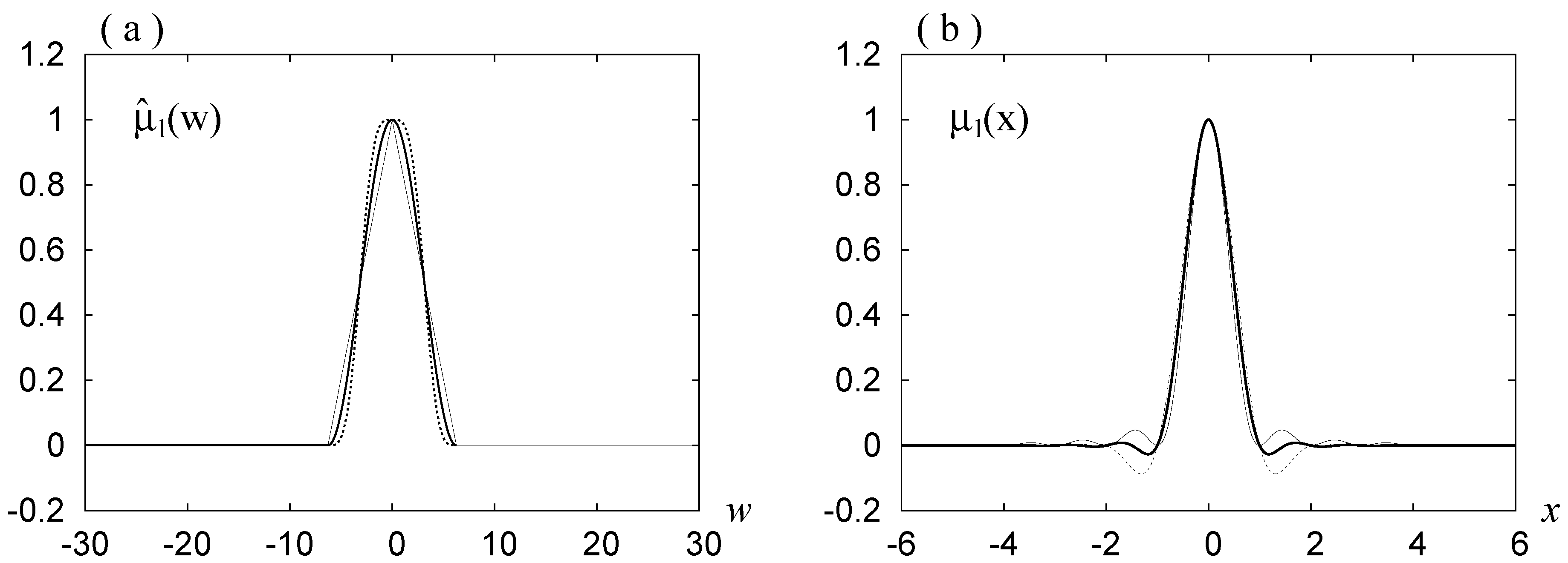
Figure 2.
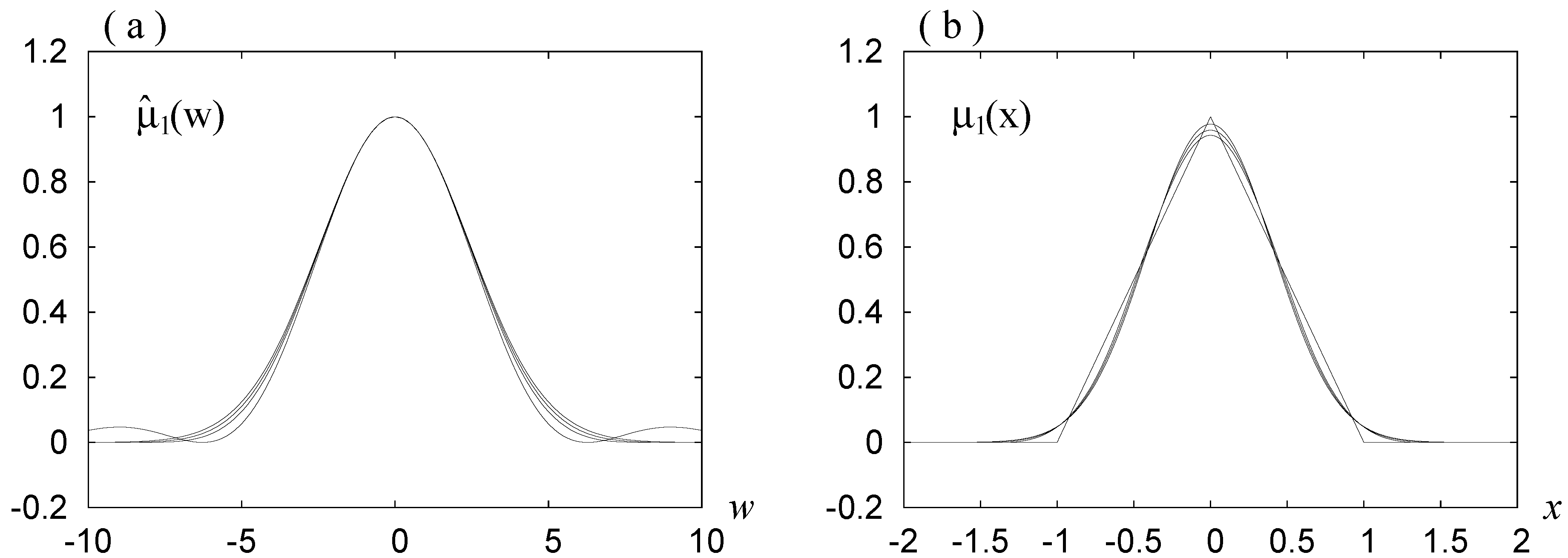
(a) for the mollifiers based on the rdH-wavelet with , and (b) those based on the scaled B-spline wavelets of order , 2. In (a), the three curves for with , 2, and 3, are shown by thin solid, thick solid, and dashed lines, respectively. In (b), two curves almost overlap. is also drawn both in (a) and in (b).
Figure 2.
(a) for the mollifiers based on the rdH-wavelet with , and (b) those based on the scaled B-spline wavelets of order , 2. In (a), the three curves for with , 2, and 3, are shown by thin solid, thick solid, and dashed lines, respectively. In (b), two curves almost overlap. is also drawn both in (a) and in (b).

Figure 3.
and for the mollifiers based on the scaled B-spline wavelets of order , 2, 4, ∞. The curves take greater values as m increases at in (a), and at and in (b).
Figure 3.
and for the mollifiers based on the scaled B-spline wavelets of order , 2, 4, ∞. The curves take greater values as m increases at in (a), and at and in (b).
Lemma 4
If Requirement 2 is satisfied for , which appears in Definition 1, then and hence .
3.1. Rapidly Decaying Harmonic Wavelets
We consider rapidly decaying harmonic (rdH-) wavelets, which were presented in [4,5]. We assume that , and that is given by
Here is assumed to satisfy the conditions that , , and for .
Lemma 5
thus defined satisfies Condition 1.
A proof of this lemma is given in Appendix A.
As for , we use for , which are given by
Lemma 6
For the mollifiers based on the rdH-wavelets, Requirement 1 is satisfied.
Proof.
This follows from and Equation (23). ☐
Remark 3
Remark 4
If we put in Equation (23), , and then . This corresponds to truncation of Fourier series, and hence we expect the Gibbs phenomenon to occur if takes nonzero values at .
Figure 1 and Figure 2a show the graphs for . In [7], it was argued that the use of and corresponds to the use of Fejer’s sum in the Fourier series, where the Gibbs phenomenon does not appear but the convergence is not good. The curve for in Figure 1b shows that Requirement 2 is satisfied, and the corresponding curve in Figure 2a shows a poor convergence. The last demerit is due to the bumps outside the main peak for this case in seen in Figure 1b.
3.2. B-Splines
The scaling function of the Haar wavelet is given by
We construct for from this by
This m is shifted by 1 from ([6] [p. 48]). is called the B-spline of order m.
Use of for , and corresponds to use the Haar, the unorthogonalized (uo-) Franklin, and the uo-Battle–Lemarie wavelet ([6] [p. 40, p. 48]), respectively.
We here define a shifted Haar wavelet, by its scaling function given by
We now construct for from by
Adopting , is given by
and hence . In particular, when , we have , where
When , we have , where
as seen in ([11] [Section 4.1]).
Lemma 7
For the mollifiers based on the B-splines, , for which Requirement 2 is satisfied.
Proof.
This follows from the fact that for all and by its construction. ☐
In [7], the choice was studied. It was noted that the Gibbs phenomenon does not occur and noise is reduced well, though not very well. In Section 4, we adopt this as Mollifier 2.
Remark 5
In [7], the method of Lanczos’ σ-factor and its multiple applications ([8] [p. 109ff, p. 132]) are called attention as a method of suppressing the Gibbs phenomenon in the Fourier series. It was noted there that Lanczos’ method corresponds to the present method using as the mollifier. Then is given by Equation (28), and hence noise reduction is not expected by Requirement 1. The extensions of Lanczos’ method correspond to the present method using for as the mollifier. Using and corresponds to the present studies for and .
3.3. Scaled B-Splines
In Section 3.2, the use of or for is mentioned. Then , and as a probability density function (pdf), it has the variance , by Equation (29) and the theory of probability. In comparing two choices of , it is desirable that the variances of them are equal or nearly equal with each other, in the respect of Requirement 3.
For , we now adopt or , so that or . Then we have , where
Now .
By the central limit theorem, as , approaches the Gaussian pdf with the variance , so that, in this limit,
If we adopt for , in the limit of , we have
In Figure 3a,b, the graphs of and , calculated by and Equations (30)–(33), are shown for , 2, 4 and ∞. The curves for are not drawn. These are between the curves for and those for , and are very close to those for . The curves of are shown for and 2 in Figure 2b.
Figure 3a shows that Requirement 1 is well satisfied by the curves for . Figure 3b shows that Requirement 2 is satisfied by all the curves, and that Requirement 3 is satisfied slightly better by the curve for . The estimations for the curves for are nearly equal, but the best of them is for . In Section 4, we adopt this as Mollifier 3.
4. Numerical Computation
We are interested in numerically calculating a function that approximates . The given data are the value of λ and a function involving noise, in place of f. We adopt as an approximation of , where . In order to calculate , we only have to choose a mollifier and a value of the scale ν. The estimations in Section 2.2 guarantee that the error can be made small if the error is small. What we can practically do is to do the calculation for a number of values of ν and to choose a reasonable one among them. We show some results of such an experiment for .
In the numerical calculations, we choose sufficiently large values and , and consider discrete values of coordinates for . The integral of a function f is approximated by , where ; See Appendix B.
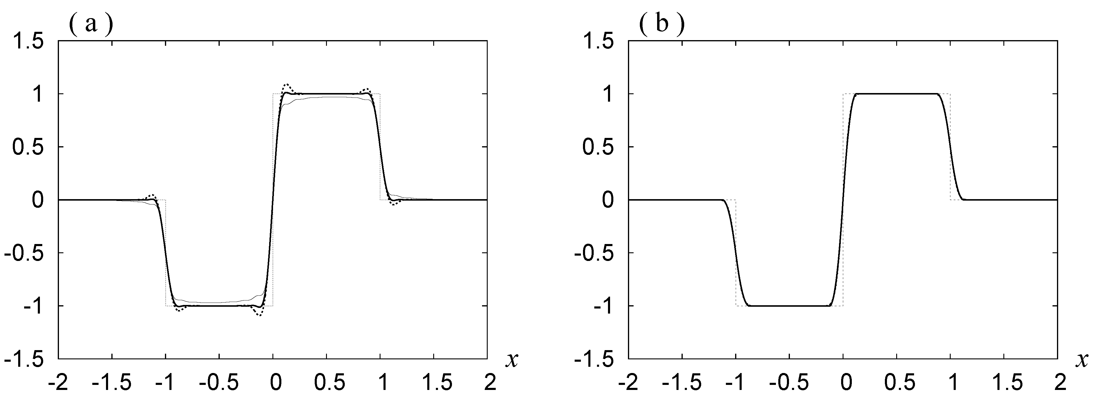
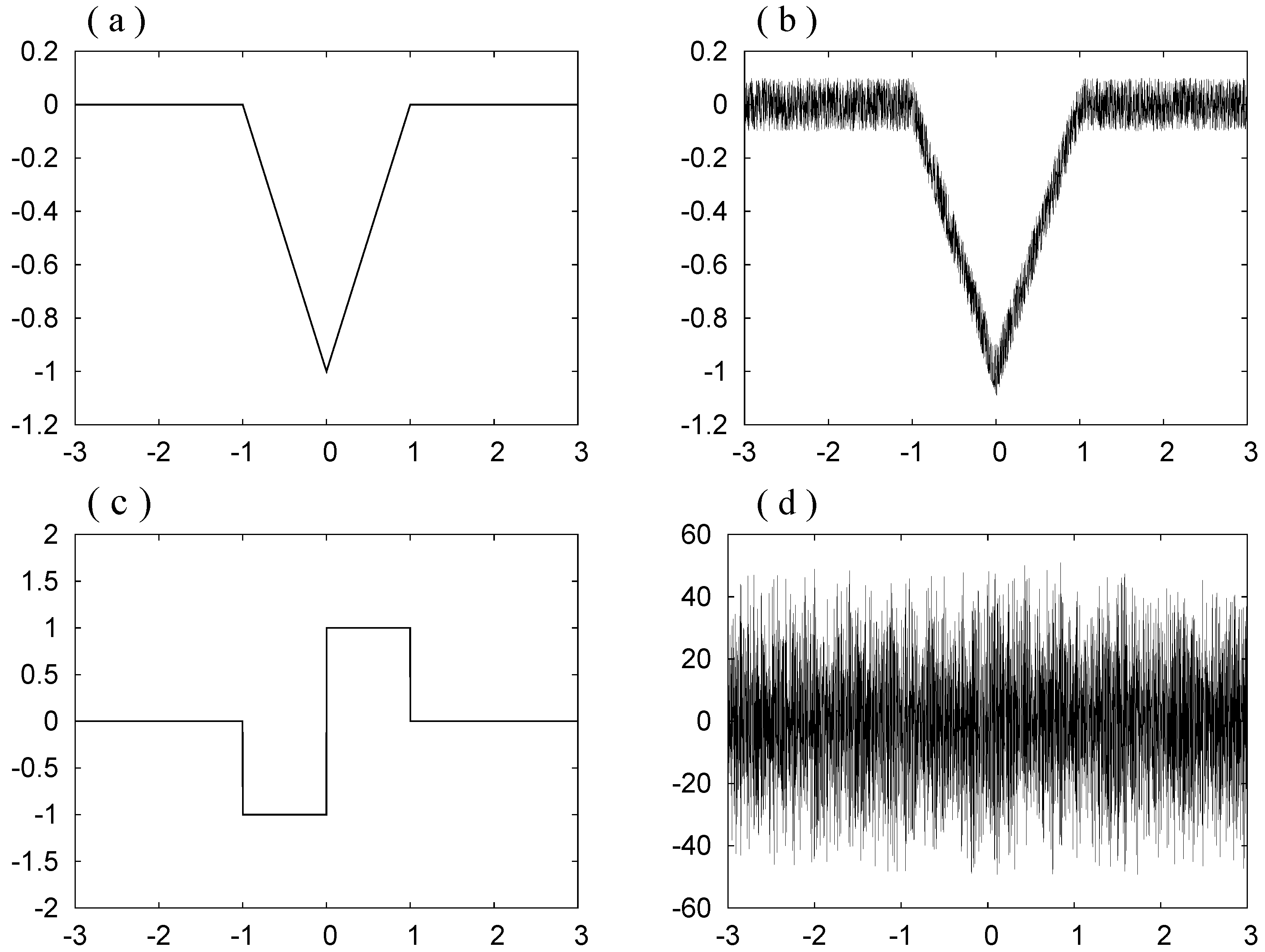
We now consider the V-shaped function , which is given by
and noisy data for , where for each k is a random number chosen from the uniform distribution in the interval . In Figure 4a,b, the functions and are shown. Figure 4c,d shows and the central difference approximate given by
We calculate by
where we put for . This quantity is differentiable and its derivative is denoted by .
Mollifier 1
The mollifier based on the rdH-wavelet using and , given by Equation (25) in Section 3.1, where and .
Mollifier 2
The mollifier based on the Haar wavelet, given by in Section 3.2, where is given by Equation (31), and and .
Mollifier 3
The mollifier based on the scaled uo-Franklin wavelet, given by in Section 3.3, where is given by (33) and (32), and and .
Figure 4.
(a) ; (b) ; (c) ; (d) .
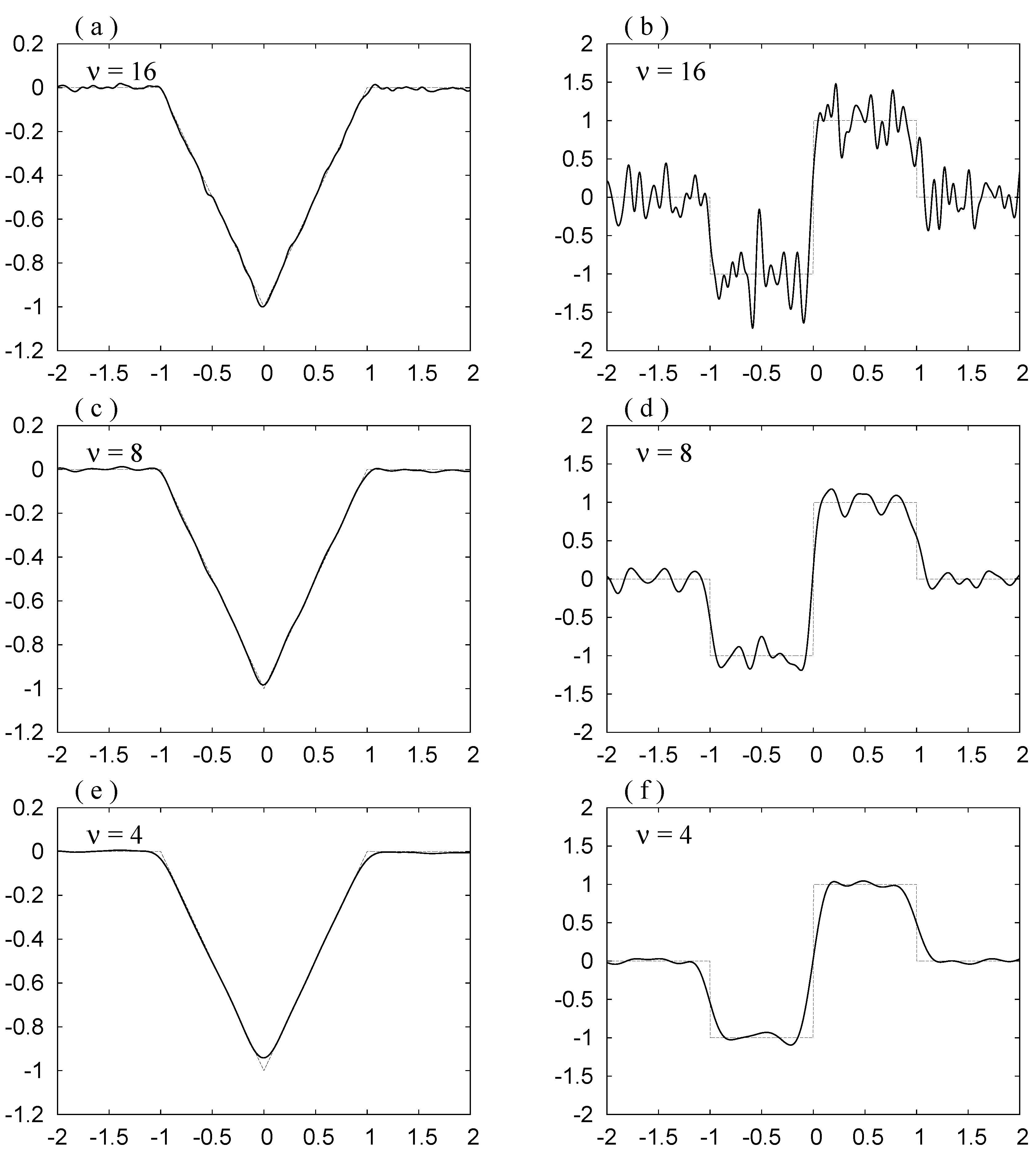
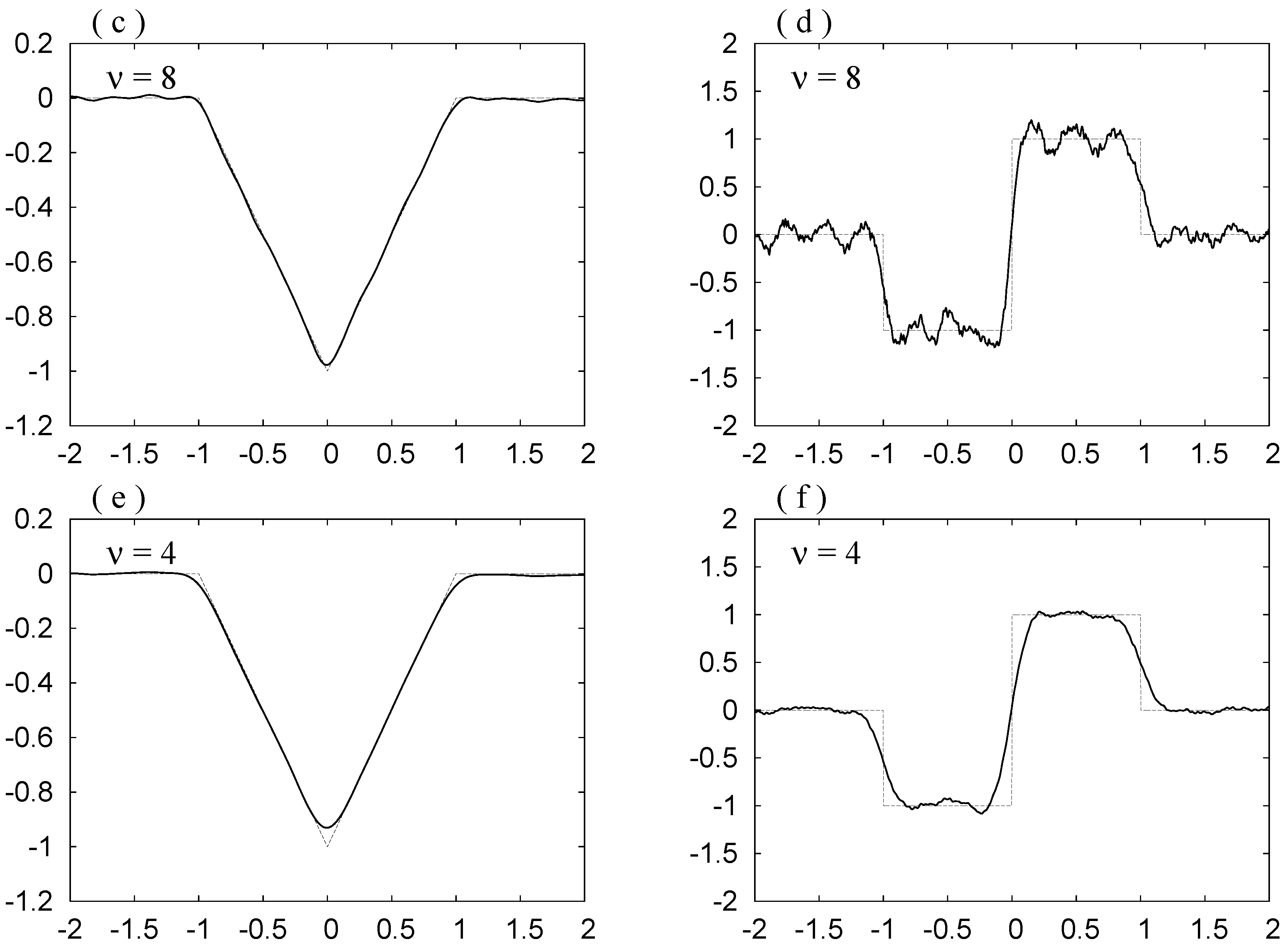
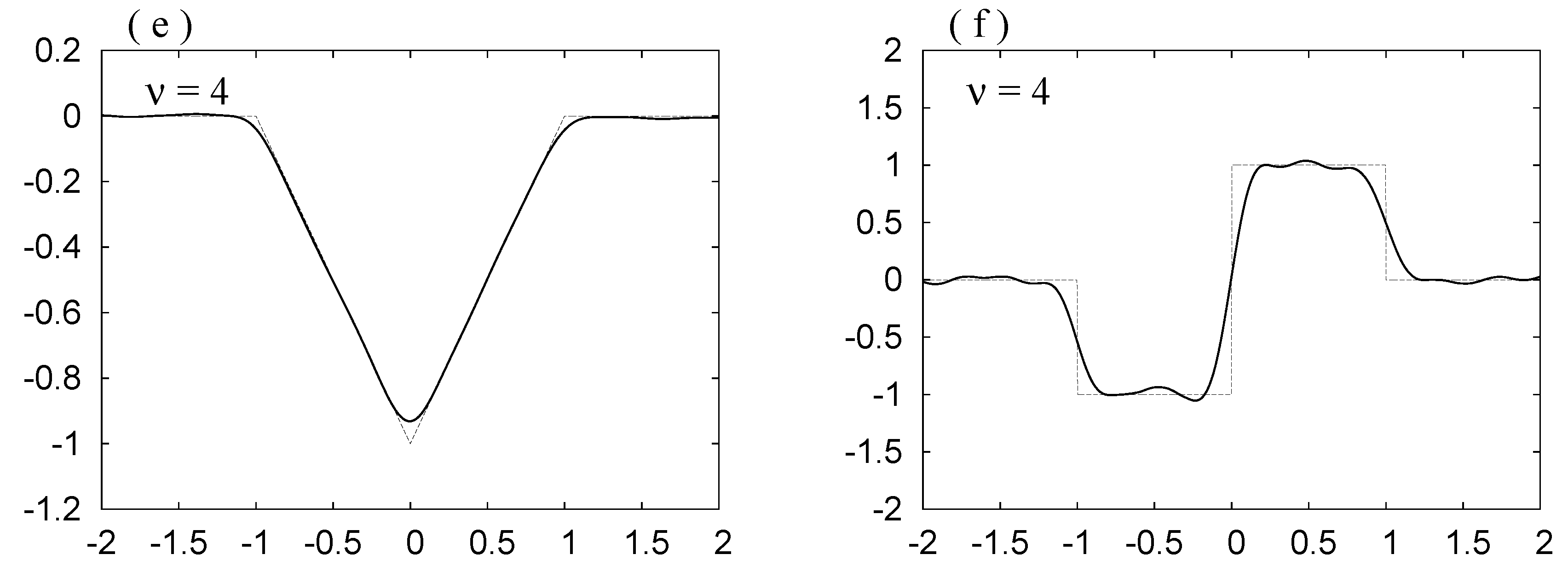
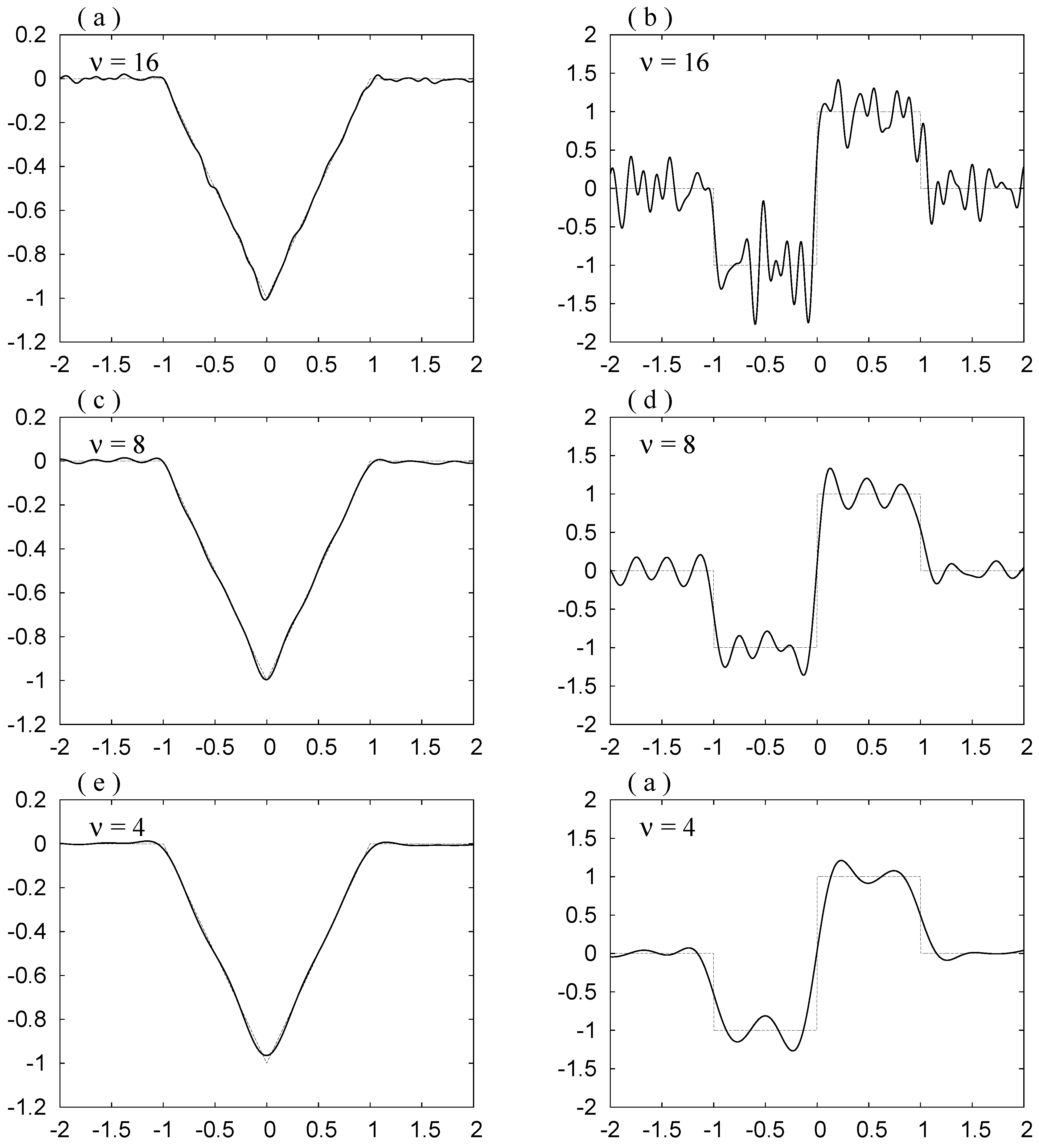
Here denotes the variance of the mollifier. In each of Figure 5, Figure 6 and Figure 7, (a) and (b) are for , (c) and (d) are for , and (e) and (f) are for . We do not observe the Gibbs phenomenon in these curves. The noise is reduced as ν decreases.
As ν decreases, the noise is depressed, but also the bottom in (a), (c) and (e) becomes rounder, and the slope at in (b), (d) and (f) becomes smaller. Hence in order to see the original forms shown in Figure 4a,c clearly, we have to draw the curves for , and . By Requirement 3, this smearing is governed by the width of the mollifier . The width may be estimated by the value of the standard deviation σ. The value is slightly smaller for the first choice.
When we compare Figure 5, Figure 6 and Figure 7, we do not observe difference between Figure 5 and Figure 7. In Figure 6, we observe that the noise reduction is not so good as in the other two.
In Figure 8, we show the curves for the choice specified by and for the rdH-wavelet. In this case, the Gibbs phenomenon is clearly seen, which is expected in Remark 3.
Figure 5.
(a), (c), (e): , ; (b), (d), (f): and , for Mollifier 1. The thinner curves show and .

Figure 6.
(a), (c), (e): , ; (b), (d), (f): and , for Mollifier 2. The thinner curves show and .
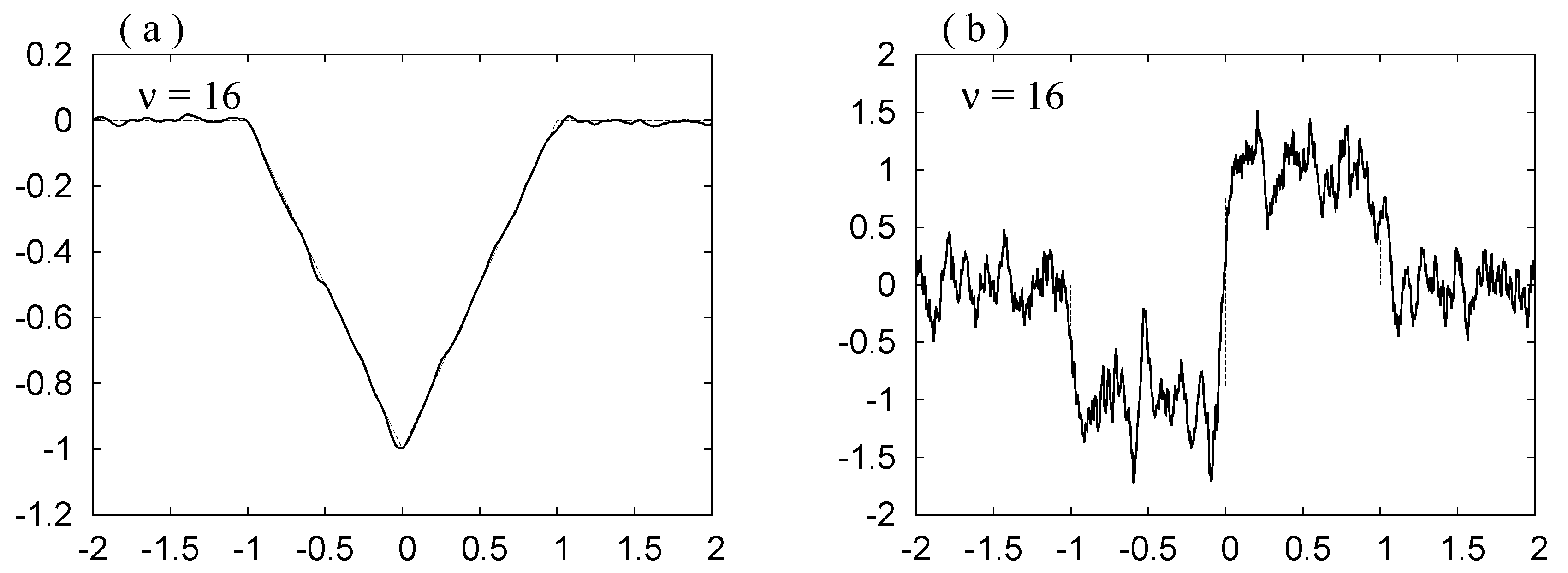

Figure 7.
(a), (c), (e): , ; (b), (d), (f): and , for Mollifier 3. The thinner curves show and .
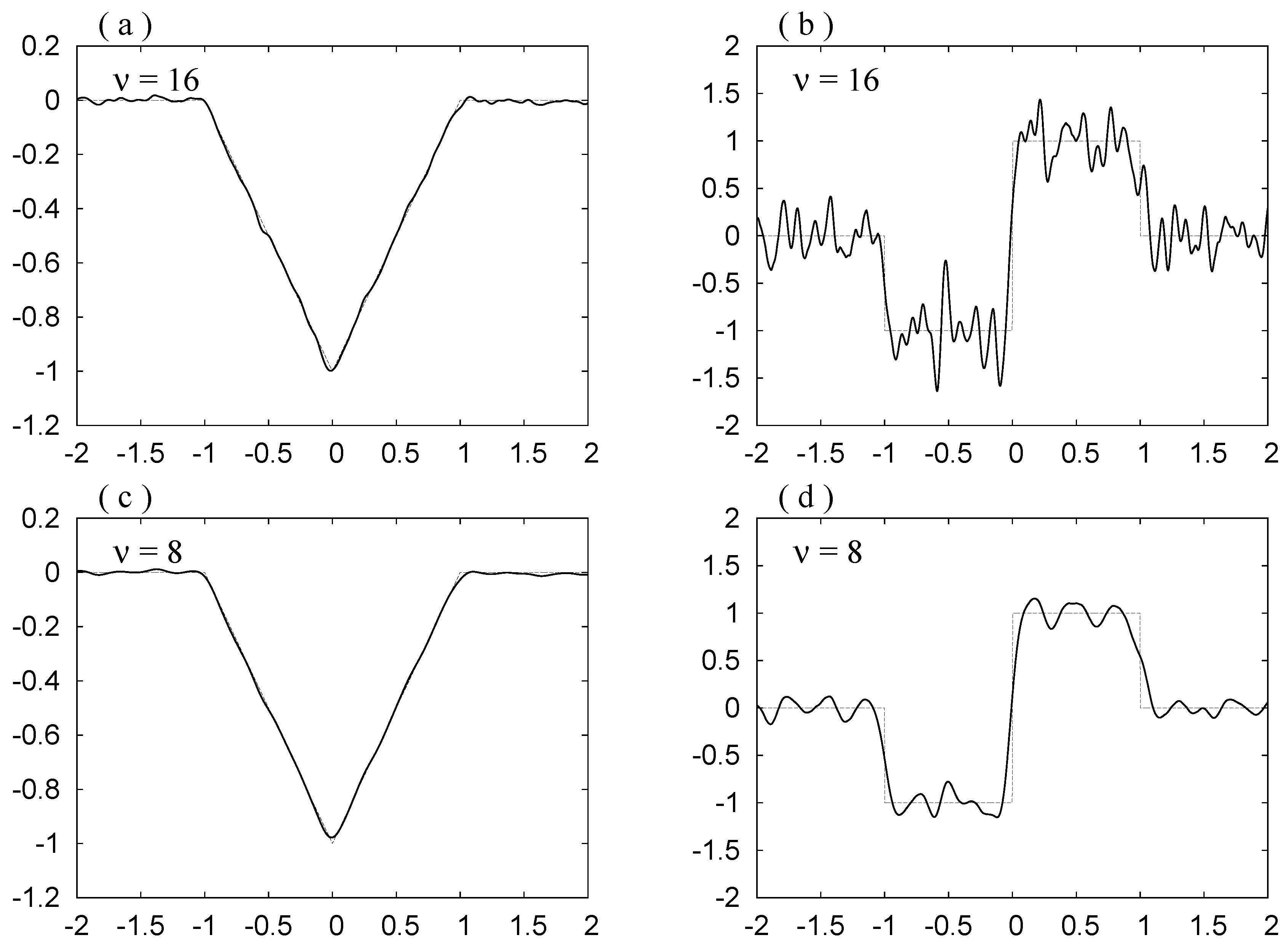

Figure 8.
(a), (c), (e): , ; (b), (d), (f): and , for the mollifier based on the rdH-wavelet using and . The thinner curves show and .
Figure 8.
(a), (c), (e): , ; (b), (d), (f): and , for the mollifier based on the rdH-wavelet using and . The thinner curves show and .

5. Concluding Remarks
In Section 4, we study three mollifiers called Mollifiers 1, 2 and 3. In [3], propositions are given for estimating the fractional derivative of a function, when the function given involves noise. Noting that those propositions are not applicable to the three mollifiers, we present revised propositions in Section 2. We here note that the new estimations are applicable to the three mollifiers.
We first confirm that Condition 3 is applicable to Mollifiers 1, 2 and 3, by choosing β satisfying , and , respectively. We next confirm that the conditions , in Propositions 1 and 2 are satisfied if λ satisfies , and , respectively, for Mollifiers 1, 2 and 3.
The last fact for Mollifier 2 is confirmed by noting that exists only when for given by Equation (31), since we then have
The corresponding calculation for Mollifier 3 is done by using with the aid of Equation (32).
In the present method of mollification, we remove high frequency component of data, regarding it to be noise. Hence if noise involves low frequency component, it will not be removed, and if high frequency component in the data is not desired to be erased, the present method will not be useful.
In the present paper, we study an example of calculating the first order derivative. In [3], the derivative of order is calculated as an example, where the mollification based on an orthogonal rapidly decaying wavelet is used.
Acknowledgements
The authors are grateful to the reviewers for helpful comments and valuable suggestions. With the help of them, the authors could improve the descriptions in this paper.
Appendices
A. Proof of Lemma 5
We denote for . Condition 1 states that for . By using Equation (23) and , we prove this as follows.
B. Use of Discrete Fourier Transform (DFT)
In ([12] [Section 12.1]), description is given on the discrete Fourier transform (DFT) and its inverse. It is assumed that N data for are given. Then the DFT of for is introduced by the first of the following equations:
The second equation represents by the inverse DFT. In ([12] [Section 12.2]), the fast Fourier transform (FFT) algorithm is presented for the numerical computation of from , and vice versa.
In the present paper, we choose two integers and , and put . For a function , we consider N values at for . Then is assumed to be a periodic series of k with period N. We now put
where . Then and are periodic series of k and n with period N, and the formulas in (B.1) are reduced to
where and . By this definition, is a periodic series of n with period N.
References
- Murio, D.A. The Mollification Method and the Numerical Solution of Ill-posed Problems; J. Wiley: New York, NY, USA, 1993. [Google Scholar]
- Hào, D.N.; Reinhardt, H.J.; Seiffarth, F. Stable numerical differentiation by mollification. Numer. Funct. Anal. Optim. 1994, 15, 635–659. [Google Scholar] [CrossRef]
- Morita, T.; Sato, K. Mollification of fractional derivatives using rapidly decaying harmonic wavelet. Fract. Calc. Appl. Anal. 2011, 14, 284–300. [Google Scholar] [CrossRef]
- Morita, T. Rapidly decaying harmonic wavelet expansion. Interdiscip. Inf. Sci. 2008, 14, 89–101. [Google Scholar] [CrossRef]
- Morita, T.; Kaneko, M. Harmonic wavelet analysis of sound. Interdiscip. Inf. Sci. 2008, 14, 245–253. [Google Scholar] [CrossRef]
- Walter, G.G.; Shen, X. Wavelets and Other Orthogonal Systems, 2nd ed.; Chapman & Hall/CRC: Boca Raton, FL, USA, 2001. [Google Scholar]
- Morita, T.; Sato, K. Mollification of the Gibbs Phenomenon Using Orthogonal Wavelets. In Proceedings of the Multimedia Technology (ICMT), 2011 International Conference, Hangzhou, China, 26–28 July 2011; Volume 7, pp. 6441–6444.
- Hamming, R.W. Digital Filters; Dover Publications Inc.: Mineola, NY, USA, 1998. [Google Scholar]
- Morita, T.; Sato, K. Analyticity and Asymptotics of Fractional Differintegrations. In preparation.
- Friedlander, G.; Joshi, M. Introduction to the Theory of Distributions, 2nd ed.; Cambridge U.P.: Cambridge, UK, 1998. [Google Scholar]
- Chui, C.K. An Introduction to Wavelets; Academic Press, Inc.: New York, NY, USA, 1992. [Google Scholar]
- Press, W.H.; Teukolsky, S.A.; Vertterling, W.T.; Flannery, B.P. Numerical Recipes, 3rd ed.; Cambridge U.P.: Cambridge, UK, 2007. [Google Scholar]
© 2013 by the authors licensee MDPI, Basel, Switzerland. This article is an open access article distributed under the terms and conditions of the Creative Commons Attribution license ( http://creativecommons.org/licenses/by/3.0/).
Share and Cite
MDPI and ACS Style
Morita, T.; Sato, K.-i. Mollification Based on Wavelets. Axioms 2013, 2, 67-84. https://doi.org/10.3390/axioms2020067
AMA Style
Morita T, Sato K-i. Mollification Based on Wavelets. Axioms. 2013; 2(2):67-84. https://doi.org/10.3390/axioms2020067
Chicago/Turabian StyleMorita, Tohru, and Ken-ichi Sato. 2013. "Mollification Based on Wavelets" Axioms 2, no. 2: 67-84. https://doi.org/10.3390/axioms2020067