Ricci Curvature on Polyhedral Surfaces via Optimal Transportation

1
ENS de Lyon, 15 parvis René Descartes - BP 7000 69342 Lyon Cedex 07, France
2
Université Paris-Est, LAMA (UMR 8050), Marne-la-Vallée F-77454, France
*
Author to whom correspondence should be addressed.
Axioms 2014, 3(1), 119-139; https://doi.org/10.3390/axioms3010119
Submission received: 27 January 2014
/
Revised: 17 February 2014
/
Accepted: 18 February 2014
/
Published: 6 March 2014
(This article belongs to the Special Issue Discrete Differential Geometry and Its Applications to Imaging and Graphics)
Abstract
:The problem of correctly defining geometric objects, such as the curvature, is a hard one in discrete geometry. In 2009, Ollivier defined a notion of curvature applicable to a wide category of measured metric spaces, in particular to graphs. He named it coarse Ricci curvature because it coincides, up to some given factor, with the classical Ricci curvature, when the space is a smooth manifold. Lin, Lu and Yau and Jost and Liu have used and extended this notion for graphs, giving estimates for the curvature and, hence, the diameter, in terms of the combinatorics. In this paper, we describe a method for computing the coarse Ricci curvature and give sharper results, in the specific, but crucial case of polyhedral surfaces.
Classification:
MSC 05C10; 68U05; 90B061. The Coarse Ricci Curvature of Ollivier
Defining the concept of curvature in the discrete setting, as it exists on smooth manifolds, has been, and still is, a challenging goal, both for theoretical and applied purposes. Whether a discrete analog is meaningful or not lies in the geometric properties one can recover, such as diameter estimates (Myers’ theorem below), isoperimetric or functional inequalities [1], topological properties (e.g., Gauss–Bonnet, Hodge theorem), spectral properties [2,3] or the limit behavior for discretizations. In the intrinsic case (the case of extrinsic curvature and, in particular, discretized surfaces in three-space goes beyond the presented paper, and we refer the reader to [4], for instance.), the angular defect and its counterpart for graphs, the combinatorial curvature (see [1,5,6]) play the role of the Gaussian (or scalar) curvature. Ricci curvature, however, is different in that it is a directional quantity, attached to a point and a tangent vector; therefore, a discrete analog would be edge-based. The earliest attempt at defining a combinatorial Ricci curvature comes from Stone [7,8], who implements Myers’ proof on Jacobi fields in order to get a diameter bound. Forman [9] later defined Ricci curvature by means of the decomposition of the Laplace operator analogous to the Bochner–Weitzenböck formula on smooth manifolds, also deriving a Myers-type theorem. More recently, the methods from probability theory and optimal transportation have made new inroads into smooth and discrete (metric) geometry. This new field is wide and thriving, and we will not attempt to describe it ( In particular, we will leave out the so-called curvature-dimension inequalities; see [10,11].). Rather, we will focus on a surprising notion defined by Ollivier, which we will eventually compare to Forman’s.
Let us first recall the definition of the coarse Ricci curvature, as given originally by Ollivier in [12]. Since our focus is on polyhedral objects, we will use, for greater legibility, the language of graphs and matrices, rather than more general measure theoretic formulations. In this section, we will assume that our base space is a simple graph (no loops, no multiple edges between vertices), unoriented and locally finite (vertices at finite distance are in finite number) for the combinatorial distance (the length of the shortest chain between x and ):
where stands for the adjacency relation and adjacent vertices are at distance 1. We shall call this distance the uniform distance; the more general case will be considered in Section 4. Polyhedral surfaces (also known as two-dimensional cell complexes) studied afterwards will be seen as a special case of graphs (specifically, they obey the assumption in [1]). We do not require our graphs to be finite, but we will nevertheless use vector and matrix notations (with possibly infinitely many indices).
For any , a probability measure, μ on X, is a map, , such that . Assume that for any vertex, x, we are given a probability measure, . Intuitively, is the probability of jumping from x to y in a random walk. For instance, we can take to be the uniform measure on the sphere (or one-ring) at x, , namely if , where denotes the degree of x and zero elsewhere. A coupling or transference plan ξ between μ and is a measure on , whose marginals are , respectively:
Intuitively, a coupling is a plan for transporting a mass of one distributed according to μ to the same mass distributed according to . Therefore, indicates which quantity is taken from y and sent to . Because mass is nonnegative, one can only take from x the quantity, , no more no less, and the same holds at the destination point, ruled by . We may view measures as vectors indexed by V and couplings as matrices, and we will use that point of view later.
The cost of a given coupling ξ is:
where cost is induced by the distance traveled. The Wasserstein distance, , between probability measures is:
where the infimum is taken over all couplings, ξ, between μ and (such a set will never be empty, and we will show that its infimum is attained later on). Let us focus on two simple, but important examples:
- (1)
- Let be the Dirac measure, , i.e., equals one when and zero elsewhere. Then, there is only one coupling, ξ, between and , and it satisfies if and and vanishes elsewhere. Obviously, .
- (2)
- Consider now , the uniform measures on unit spheres around x and , respectively; then, a coupling, ξ, vanishes on , whenever y lies outside the sphere, , or outside . So the (a priori infinite) matrix, ξ, has at most nonzero terms, and we can focus on the submatrix, , whose lines sum to and columns to . For instance, ξ could be the uniform coupling:where we have written only the submatrix.
- (3)
- A variant from the above measure is the measure uniform on the ball .
Ollivier’s coarse Ricci curvature (also called Wasserstein curvature) between x and (which, by the way, need not be neighbors) measures the ratio between the Wasserstein distance and the distance. Precisely, we set:
Since is the uniform measure on the sphere, then compares the average distance between the spheres, and , with the distance between their centers, which indeed depends on the Ricci curvature in the smooth case (see [12,13] for the analogy with Riemannian manifolds, which prompted this definition).
We will rather use the definition of Lin, Lu and Yau [14] (see also Ollivier [13]) for a smooth time variable, t: let be the lazy random walk:
so that interpolates linearly between the Dirac measure and the uniform measure on the sphere (in [14], a different notation is used: the lazy random walk is parametrized by , and the limit point corresponds to ). We let and as . We then set:
and we will call the (asymptotic) Ollivier–Ricci curvature. The curvature, , is attached to a continuous Markov process, whereas corresponds to a time-discrete process (however, both approaches are equivalent, by considering weighted graphs and allowing loops ( i.e., weights ). See [2] and also §4 for weighted graphs). Lin, Lu and Yau [14] prove the existence of the limit, , using concavity properties. In the next section, we give a different proof by linking the existence to a linear programming problem with convexity properties.
The relevance of such a definition comes from the analogy with Riemannian manifolds, but can also be seen through its applications, e.g., the existence of an upper bound for the diameter of X depending on (see Myers’ theorem below).
2. A Linear Programming Problem
In the case of graphs, the computation of is surprisingly simple to understand and implement numerically. Recall that a coupling, , between and is completely determined by a submatrix, and henceforward, we will identify with this submatrix. A coupling is actually any matrix in with nonnegative coefficients, subject to the following t-dependent linear constraints: and , for all and , where and are the following matrices:
is the standard inner product between matrices and denotes the transpose of M. We will write the nonnegativity constraint, , where is the basis matrix, whose coefficients all vanish, except at . The set of possible couplings is therefore a bounded convex polyhedron, , contained in the unit cube . In the following, we will also need the limit set , which contains a unique coupling (see Case 1 above).
In order to compute , we want to minimize the cost function, c, which is actually linear:
where D stands for the distance matrix restricted to , so that D is the (constant) gradient of c. Clearly, the infimum is reached, and minimizers lie on the boundary of . Then, either the gradient D is perpendicular to some facet of . The minimizer can be freely chosen on that facet, or not, and the minimizer is unique and lies on a vertex of . Moreover the Kuhn–Tucker theorem ([15], part VI) gives a characterization of minimizers in terms of Lagrange multipliers (a.k.a. Kuhn–Tucker vectors): minimizes c on if and only if there exists , and , such that:
and:
meaning that the Lagrange multipliers, , have to vanish unless the inequality constraint is active (or saturated): . As a consequence: (i) finding a minimizer is practically easy thanks to numerous linear programming algorithms; and (ii) proving rigorously that a given is a minimizer requires only writing the Relations (1) and (2) for .
The non-uniqueness is quite specific to the metric, when cost is proportional to length and, therefore, linear instead of strictly convex (instead of, say, length squared as in the 2-Wasserstein metric, ). It corresponds to the following geometric fact: transporting mass m from x to z is equivalent in cost to transporting the same mass, m, from x to y and from y to z, as long as y is on a geodesic from x to z (and , since we prohibit negative mass).
Computing the Olivier–Ricci curvature requires a priori taking a derivative; however, it is actually much simpler, due to the following lemma, which also proves its existence, without the need for subtler considerations, like in [14]:
Lemma 1.
For small enough, convex sets and are homothetic. More precisely,
Proof.
First, write the constraint corresponding to the lazy random walk as , where and iff . Let lie in and be positive. Then, lies in . Indeed:
We see immediately that whenever . Moreover, , provided . All the previous arguments hold in generality, but the nonnegativity of needs a different argument when . Because and are probability measures, , and for any t,
consequently:
Hence, for , is positive for any matrix, , satisfying the equality constraints (and the same holds for , using again that ).
The significance of this positivity is that the constraint is never saturated; there will always be some mass transported from x to if t is small enough, because the other vertices cannot hold all the mass from x. ☐
Remark 1.
The lemma holds true for small enough, as long as is uniformly bounded on X, a property that we will meet later. Equation (3) generalizes, and we see easily that if , then the homothety property holds for all .
Proposition 2.
The Ollivier–Ricci curvature, , is equal to any quotient for t small enough (e.g., ).
Proof.
As a consequence of Lemma 1, the gradient, D, has the same projection on the affine space determined by the equality constraints, and the minimizers can be chosen to be homothetic for small enough. If denotes this family of homothetic minimizers:
So, is linear for t small enough and:
As a consequence, computing is quite simple: one needs only solve the linear problem for t small enough (e.g., ).
Remark 2.
This property linking the time-continuous Olivier–Ricci curvature to the time-discrete curvature is true in generality, as soon as the random walk is lazy enough, i.e., the probability of staying at x is large enough (see the remark of Ollivier [12] at the end of Section 1.1, [16] for time-continuous and space-discrete Markov chains with exponential jump times and, also, [17] for more details on Ollivier–Ricci curvature in the continuous case).
Finally, we note that this optimization problem is an instance of integer linear programming, and as a consequence, the solution is integer-valued up to a multiplicative constant:
Theorem 3.
For any pair of adjacent vertices, , with degrees , and , there exists an optimal coupling, , with coefficients in ; consequently, and lie in .
Proof.
Let us first rewrite the constraints above as the following single linear equation. Numbering and , the neighbors of x and and the neighbors of , we consider the vector . The constraints amounts to for the following data:
The integral matrix, A, is totally unimodular: Every square, non-singular submatrix, B of A, has determinant . Indeed, A satisfies the following requirements:
- the entries of A lie in ;
- A has no more than two nonzero entries on each column;
- its rows can be partitioned into two sets and , such that if a column has two entries of the same sign, their rows are in different sets.
In our setting, choose , so that the coefficients of b lie in . By the above remarks, so do the coefficients of , since an optimal coupling can be chosen to be a vertex of the constraint set. Since the distance matrix is also integer-valued, the cost, , lies in , and for two neighbors, , . The curvature is obtained by diving by , hence the result. The reasoning also holds for . ☐
3. Curvature of Discrete Surfaces
Estimates for the Ollivier–Ricci curvature are given in [11,14] ( in the first paper, in the second) for general graphs and for some specific ones, such as trees. Essentially, they rely on studying one coupling, which gives an upper bound on , hence a lower bound on the curvature, which may or may not be optimal. We will give below exact values, albeit in the specific setting that concerns us: polyhedral surfaces. Furthermore, we will always assume that vertices are neighbors; in other words, we see as a function on the edges. Actual computing of for more distant vertices is, of course, possible, but much more complicated. However, it should be noted that trivially enjoys a concavity property, as a direct consequence of the triangle inequality on the distance, : if is a geodesic path from x to , then:
the latter equality holding only in the uniform metric, because between neighbors. This inequality passes to the limit and applies to , as well. The concavity property implies in particular that if is bounded below on all edges, then has the same lower bound on all couples, .
We use this fact to give a trivial proof of Myers’ theorem (see also [19] for the smooth case).
Theorem 4
(Ollivier [12], prop. 23). If is bounded below on all edges by a positive constant, ρ, then S is finite, and its diameter is bounded above by .
Proof.
Using the triangle inequality again on :
where is the jump at x, which is also the expectation, , of the distance to x with respect to the probability, . For the uniform metric , so that:
which gives the upper bound for the diameter. Since S is locally finite, it is therefore finite. ☐
We will now give our results and compare them with those obtained either by Jost and Liu [11] or by using Forman’s definitions of Ricci curvature [9].
As the first example, let us give the Ollivier–Ricci curvature for the Platonic solids (with as a comparison, corresponding to the non-lazy random walk) in Table 1:

Table 1.
Ollivier–Ricci (asymptotic and discrete at time 1 for the Platonic solids, along Forman’s version of Ricci curvature (divided by three, to be comparable). Values in bold are sharp with respect to Myers’ theorem.
| Tetrahedron | Cube | Octahedron | Dodecahedron | Icosahedron | |
|---|---|---|---|---|---|
| 0 | |||||
| 0 | |||||
| Forman | 0 | 0 |
This stresses the difference between (used in [11]) and , which exhibits, in our opinion, a more geometric (and less graph-theoretic) behavior. In particular, the values of are sharp with respect to Myers’ theorem for the cube and the octahedron. Forman refers to the combinatorial Ricci curvature for unit weights defined in [9], which also satisfies a Myers’ theorem, albeit with a different constant: the diameter is bounded above by , hence our choice to divide it by three, to allow comparison between with the Ollivier–Ricci curvature. Forman’s Ricci curvature is sharp only for the cube.
Tessellations by regular polygons fit well in this framework, since all edges have the same length. Regular tilings are the triangular, square and hexagonal tiling. The triangular tiling corresponds to the case (see Table 2 below) and has zero Ollivier–Ricci curvature, and so does the square tiling. However, the hexagonal lattice has negative Ollivier–Ricci curvature equal to .
Table 2.
Asymptotic Ollivier–Ricci curvature, , according to respective degrees of x and , compared to the Time 1 Ollivier–Ricci , as well as Forman’s Ricci curvature (divided by three for comparison purposes); refers to the estimates of Jost and Liu.
| Others | |||||||
|---|---|---|---|---|---|---|---|
The method can also be applied to semiregular tiling, but those are only vertex-transitive in general and not edge-transitive (with the exception of the trihexagonal tiling); hence, one must treat separately the different types of edges. For example, for the snub square tiling, for an edge between two triangles, but for an edge between a triangle and a square.
The results above can easily be derived using making computation by hand or by using integer linear programming software (a source file with all the above examples to be used with open source software Sage [20] is attached to the article). The next results however are of a more general nature, with variable degrees, and cannot be obtained by simple computations. We consider adjacent vertices on a triangulated surface with the following genericity hypotheses:
- (B)
- are not on the boundary;
- (G)
- for any and , there is a geodesic of length in .
Theorem 5.
Under the genericity Hypotheses (B) and (G), the Ollivier–Ricci curvature depends only on the degrees, , of vertices and is given in Table 2.
Proof.
To compute the optimal cost, , we need only find a coupling, , for which the Kuhn–Tucker relation (1) holds. Thanks to the genericity Hypothesis (G), we can restrict ourselves to finite matrices (on ). Details are given in the Section 5. Note that Hypothesis (B) makes for simpler calculations, but they could obviously be extended to deal with the presence of a boundary. Despite its incompatibility with our genericity hypotheses, we include the case for the sake of completeness. ☐
Table 2 gives and as a function of respective degrees . Because , we may assume without loss of generality that . We compare with Forman’s expression and also to the lower bound:
given by Jost and Liu [11] for general graphs, where is the number of triangles incident to the edge (), which, under our hypotheses, is always equal to two. Jost and Liu conclude that the presence of triangles improves the lower Ricci bound. We see here that when there are only triangles, one obtains an actual value, which differs from their lower bound as soon as .
Remark 3.
1. The case is given here, although it contradicts either (B) or (G), the latter being the tetrahedron computed above; similarly, the case is excluded.
- 2.
- Zero Ollivier–Ricci curvature is attained only with degrees (regular triangular tiling), and .
4. Varying Edge Lengths
While many authors have focused on the graph theory, the case of polyhedral surfaces is somewhat different: the combinatorial structure is more restrictive, as we have seen above, but the geometry is more varied. In particular, edge lengths may be different from one. This is partially achieved in the literature [11,14] by allowing weights on the edges, which amounts to changing the random walk, but we think the geometry should intervene at two levels: measure and distance. We will present here a general framework to approach the problem, using the Laplace operator, which depends on both the geometric and the combinatorial structure of S. One must also note the ambiguous definition of the Ollivier–Ricci asymptotic curvature, which plays the role of a length in Myers’ theorem, and yet, its definition makes it a dimensionless quantity. Indeed multiplying all lengths by a constant λ will not change (since is multiplied by λ, as well).
In the following, we assume that S is a polyhedral (or discrete) surface with set of vertices V, edges E and faces F. Furthermore, S is not only locally finite, but its vertices have a maximum degree, ( denotes the minimal degree, which is at least two for surfaces with boundary and three for surfaces without boundary). The geometry of S is determined by the geometry of its faces, namely an isometric bijection between each face, f, and a planar face of identical degree, with the compatibility condition that edge lengths measured in two adjacent faces coincide. Then, two natural notions of length arise: (i) the combinatorial length, which counts the number of edges along a path; and (ii) the metric length, where each edge length is given by the geometry. Each notion of length yields a different distance between vertices: the combinatorial distance, , which we have used above, and the metric distance, d. Note that if each face is assumed to be a regular polygon with edges of length one, then both distances agree, and metric theory coincides with graph theory. We will make the following assumption on the geometry: the distances, d and , are metrically equivalent: . Such a hypothesis holds if the lengths of the edges are uniformly bounded above and below; in particular, the aspect ratio is bounded (this also rules out extremely large or extremely small faces, which could happen with only the bounded aspect ratio).
We consider a differential operator, Δ (a Laplacian, see [21]) determined by its values, , for vertices and the usual properties (note that our sign convention is such that the Laplacian is a negative operator; [21] uses the opposite):
- (a)
- whenever ;
- (b)
- whenever and (locality property);
- (c)
- , which implies that (note that the sum is finite, due to the previous assumption and the local finiteness of S).
The Laplacian is not a priori symmetric, i.e., -self-adjoint (though it could be made so with respect to some metric on vertices). Thanks to the finiteness assumption (b), we can define iterates of Δ for integer k, and the coefficient (not to be confused with ) is:
the sum being taken on all paths of length k on S. By direct recurrence, we see that our boundedness hypotheses imply the bound . Indeed,
As a consequence, the heat semigroup is well defined. It acts on measures and defines the image measure of the Dirac measure at x by:
where is the lazy random walk studied above (for the harmonic Laplacian, but results hold in the general case). The random walks, , have finite first moment, as can be inferred from the proof of the following.
Proposition 6.
The Ollivier–Ricci curvature depends only on the first order expansion of the random walk:
Proof.
Consider any coupling, ξ, that transfers mass from points at (uniform) distance from x of at least two, to x and its neighbors. If the vertex, y, is at -distance k from x, then for and:
The points at uniform distance k from x are at most numerous, and using the equivalence between distances, they will be moved at most by to x or one of its neighbors:
Since:
we conclude that both limits coincide. ☐
As a consequence, it is natural to replace in the section above the random walk by , for some definition of the Laplacian (see [22,23,24]). However, in order to recover the geometric properties above, one needs to normalize the random walk, , so that the jump , i.e., the average distance of points jumping from x should be t. That amounts to setting:
equivalently, one might renormalize the Laplacian accordingly. As a consequence, now behaves as the inverse of a length, as expected. Furthermore, Myers’ theorem 4 is still valid. Indeed, while Equation (4) no longer holds when edge lengths vary, it remains true that if is bounded below on all edges by ρ.
An example: The rectangular parallelepiped.
For the rectangular parallelepiped with edges of lengths , the Ollivier–Ricci curvature is:
along an edge of length a, and others follow (see §5.4). For the cube, we recover . If a is the length of the longest edge, an application of Myers’ theorem yields an upper bound for the diameter times greater than its actual value, .
Remark 4.
A more general theory can be developed with non-local operators, by replacing local finiteness (property (b) above) with convergence requirements. Another, still finite, natural generalization of (b) is to allow whenever x and y belong to the same face. For a triangulated manifold, this amounts to the usual neighborhood relation, but as soon as some faces have more than three edges, this makes a difference (e.g., the cube). Note, however, that the corresponding Myers’ theorem needs to be adjusted, as well, since the jump will change accordingly. In our experiments on Platonic solids with , a uniform measure on vertices of , we did not find better diameter bounds with this method.
Remark 5.
One might also be tempted to compute Ollivier–Ricci curvature on the surface, S, seen as a smooth flat surface with conical singularities (so that distances are computed between points on the faces). If vertices both have nonnegative Gaussian curvature (a.k.a. angular defect ), then by a computation analog to Ollivier’s [12], we infer:
which differs from our previous computations. This emphasizes that this setup is somewhere in between the smooth and the discrete setup.
5. Appendix: Solutions for the Linear Programming Problem on Generic Triangulated Surfaces
We give here the Lagrange multipliers for the linear programming problem and the corresponding minimizer. The regular tetrahedron is given first as an example of the method, and the main result consists of analyzing the various cases according to their (arbitrary) degrees. Cases with degrees less or equal to six can easily be computed by a machine, and we refer to the Sage program attached.
5.1. The Regular Tetrahedron
The distance matrix for Vertices 1, 2, 3 and 4 is:
and the optimal coupling from to shifts mass from Vertex 1 to Vertex 2 (provided ), leaving other vertices untouched:
with Lagrange multipliers:
the last matrix corresponding to a linear combination of with positive coefficients , only where . Conversely, it is straightforward from to deduce that is unique. Hence and . The case cannot be dealt with in the same way, but admits the following optimal transference plan:
with cost and, therefore, curvature .
Remark 6.
The case of degrees differs only in that the distance between Vertices 3 and 4 is equal to two instead of one. However, the optimal couplings found above do not move mass from 3 nor from 4. Hence, it is also optimal for the case.
5.2. Generic Triangulated Surfaces
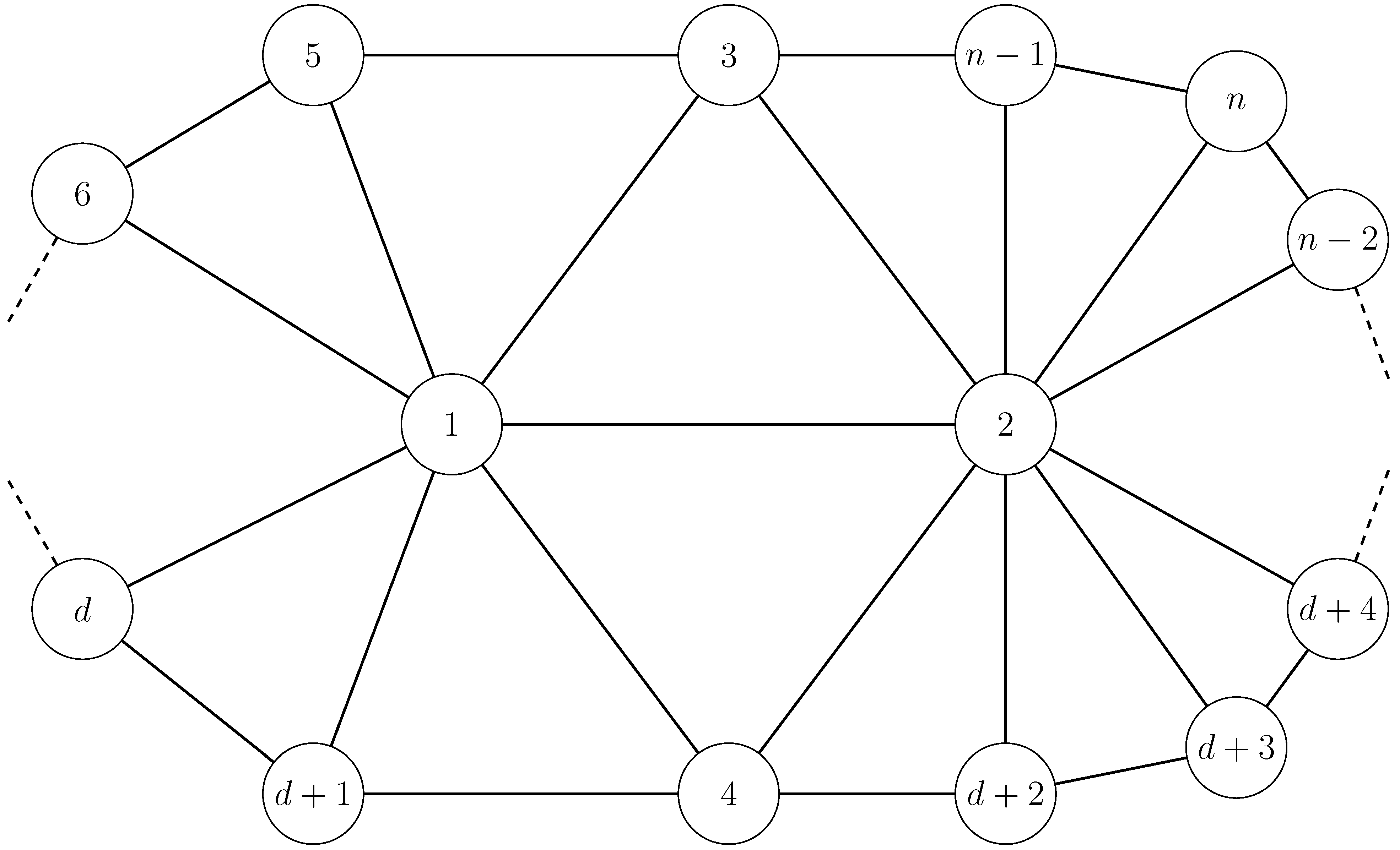
We analyze now generic triangulated surfaces according to the degrees of x and . In our matrix notation, x will have an index 1 and an index 2. Since x and are not on the boundary, all edges containing them belong to two triangular faces. In particular, there are two vertices, with indices 3 and 4, which are neighbors of both x and (see Figure 1). There remains exclusive neighbors of x (that are not neighbors of ), ordered from 5 to , along the border of , and exclusive neighbors of , ordered from to along the border of .
Figure 1.
Generic description of .

The distance matrix is:
The form of the distance matrix is somewhat different when d or are very small. Indeed, due to the genericity assumption (B), both degrees are larger or equal to 4. We see easily that the distance from an exclusive neighbor, y, of x to an exclusive neighbor, , of is in general ( i.e., for neighbors, y, and neighbors, ) obtained by a geodesic passing though x and . However, when or , “shortcuts” predominate, hence the need for ad hoc computations.
Applying the constraints, we see that any coupling, and, in particular, the optimal coupling, takes the following block form:
so, we may as well restrict to the Lines 1 through and Columns 1, 2, 3 and 4 and through of matrices D and . Then, the submatrix of D can be written (for ):
Similarly, we will write , the relevant submatrix of the coupling ξ, and .
When d and are large, the optimal coupling moves the mass mainly along the edge . This gives a general formula for values of d and . For values of , we set:
and show that Δ has only nonnegative coefficients.
- and :The distance matrix, D, has only five rows, and its submatrix is slightly different:and an optimal transportation plan is:where:with cost . Note that, thanks to , we have , so as needed.
- and :Similarly, we have:where:and the cost is . Thanks to , we have as needed.
We conclude that in all cases where , we have , as claimed.
5.3. Computation
In the case , the measure, , does not put any weight on x; hence, any transfer plan is identically zero along the line corresponding to x (and along the column corresponding to y). In our notations, it would amount to discarding the first line and the second column of all matrices previously written, but for clarity and comparison purposes, we will keep them, though they play no role. Again, we only deal with the cases of variable degree and leave the remaining cases to the computer program.
- andThe matrix, Δ, is the same as above, but because of the additional constraint, an optimal coupling is now given by:with cost . Since we need at least eight distinct lines, we cannot compute by this method anymore when .
- andAn optimal coupling is given by:
- andAn optimal coupling is given by:
- andIn this case, the Lagrange multipliers are a bit different and:An optimal coupling is given by:
5.4. The Rectangular Parallelepiped
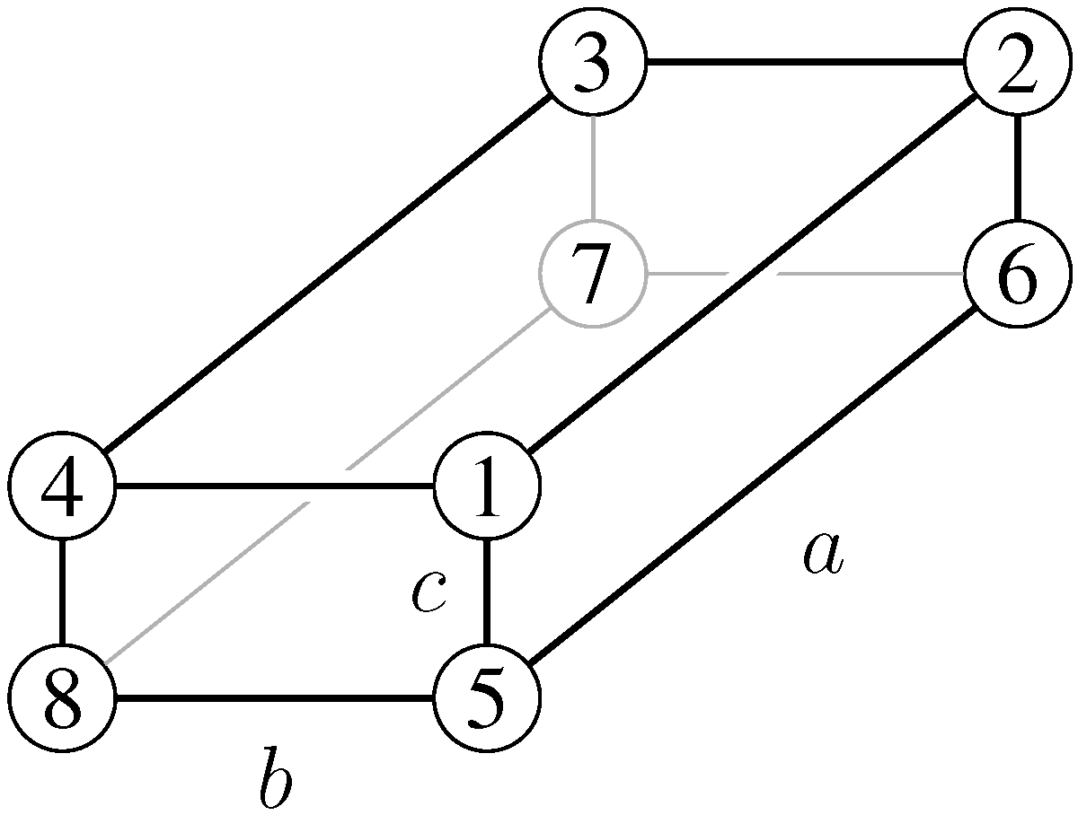
The (Delaunay) cotan Laplacian [22] for the rectangular parallelepiped with edges of lengths , , (see Figure 2) is given by:
so that ; hence we normalize to with:
The distance matrix is:
A optimal coupling is:
with cost and curvature along an edge of length a, as claimed.
Figure 2.
Rectangular parallelepiped.

Acknowledgments
The second author wishes to thank Djalil Chafaï for his stimulating remarks and for pointing out the work of Ollivier. Both authors are grateful to the referees for suggesting improvements to the article.
Author Contributions
This work was started as a master degree memoir of the first author under the direction of the second author, at the Université Paris-Est Marne-la-Vallée and later expanded by both authors.
Conflicts of Interest
The authors declare no conflict of interest.
References
- Higuchi, Y. Combinatorial curvature for planar graphs. J. Graph Theory 2001, 38, 220–229. [Google Scholar] [CrossRef]
- Bauer, F.; Jost, J.; Liu, S. Ollivier-Ricci curvature and the spectrum of the normalized graph Laplace operator. Math. Res. Lett. 2012, 19, 1185–1205. [Google Scholar] [CrossRef]
- Lin, Y.; Yau, S.T. Ricci curvature and eigenvalue estimate on locally finite graphs. Math. Res. Lett. 2010, 17, 343–356. [Google Scholar] [CrossRef]
- Morvan, J.M. Generalized Curvatures; Geometry and Computing; Springer-Verlag: Berlin, Germany, 2008; Volume 2, xii+266. [Google Scholar]
- Gromov, M. Hyperbolic groups. In Essays in Group Theory; Springer: New York, NY, USA, 1987; pp. 75–263. [Google Scholar]
- Ishida, M. Pseudo-curvature of a graph. Workshop on Topological Graph Theory, 1990. [Google Scholar]
- Stone, D.A. A combinatorial analogue of a theorem of Myers. Ill. J. Math. 1976, 20, 12–21. [Google Scholar]
- Stone, D.A. Correction to my paper: “A combinatorial analogue of a theorem of Myers”. (Ill. J. Math. 20 1976, 12–21). Ill. J. Math. 1976, 20, 551–554. [Google Scholar]
- Forman, R. Bochner’s Method for Cell Complexes and Combinatorial Ricci Curvature. Discret. Comput. Geom. 2003, 29, 323–374. [Google Scholar] [CrossRef]
- Bonciocat, A.I.; Sturm, K.T. Mass transportation and rough curvature bounds for discrete spaces. J. Funct. Anal. 2009, 256, 2944–2966. [Google Scholar] [CrossRef]
- Jost, J.; Liu, S. Ollivier’s Ricci curvature, local clustering and curvature dimension inequalities on graphs. Discret. Comput. Geom. 2014, 51, 300–322. [Google Scholar] [CrossRef]
- Ollivier, Y. Ricci curvature of Markov chains on metric spaces. J. Funct. Anal. 2009, 256, 810–864. [Google Scholar] [CrossRef]
- Ollivier, Y. A survey of Ricci curvature for metric spaces and Markov chains. In Probabilistic Approach to Geometry; Mathematical Society of Japan: Tokyo, Japan, 2010; pp. 343–381. [Google Scholar]
- Lin, Y.; Lu, L.; Yau, S.T. Ricci curvature of graphs. Tohoku Math. J. Second Ser. 2011, 63, 605–627. [Google Scholar] [CrossRef]
- Rockafellar, R.T. Convex Analysis; Princeton Landmarks in Mathematics, Princeton University Press: Princeton, NJ, USA, 1997. [Google Scholar]
- Norris, J.R. Markov Chains; Cambridge University Press: Cambridge, UK, 1998. [Google Scholar]
- Veysseire, L. Coarse Ricci curvature for continuous-time Markov processes. In arXiv.org; 2012. Available online: http://xxx.lanl.gov/abs/1202.0420v1 (accessed on 7 June 2012). [Google Scholar]
- Papadimitriou, C.H.; Steiglitz, K. Combinatorial Optimization; Algorithms and Complexity, Courier Dover Publications: Mineola, NY, USA, 1998. [Google Scholar]
- Gallot, S.; Hulin, D.; Lafontaine, J. Riemannian Geometry, 2nd ed.; Universitext, Springer-Verlag: Berlin, Germany, 1990. [Google Scholar]
- Sage computer program. Available online: http://www.sagemath.org (accessed on 6 March 2014).
- Colin de Verdière, Y. Spectres de Graphes; Société Mathématique de France: Paris, France, 1998. [Google Scholar]
- Bobenko, A.I.; Springborn, B.A. A discrete Laplace-Beltrami operator for simplicial surfaces. Discret. Comput. Geom. 2007, 38, 740–756. [Google Scholar] [CrossRef]
- Wardetzky, M.; Mathur, S.; Kälberer, F.; Grinspun, E. Discrete Laplace operators: No free lunch. In Proceedings of the ACM SIGGRAPH ASIA 2008 Courses, Singapore, Singapore, 10–13 December 2008; p. 19.
- Alexa, M.; Wardetzky, M. Discrete Laplacians on general polygonal meshes. ACM Trans. Graph. (TOG) 2011, 30, 102. [Google Scholar] [CrossRef]
© 2014 by the authors; licensee MDPI, Basel, Switzerland. This article is an open access article distributed under the terms and conditions of the Creative Commons Attribution license (http://creativecommons.org/licenses/by/3.0/).
Share and Cite
MDPI and ACS Style
Loisel, B.; Romon, P. Ricci Curvature on Polyhedral Surfaces via Optimal Transportation. Axioms 2014, 3, 119-139. https://doi.org/10.3390/axioms3010119
AMA Style
Loisel B, Romon P. Ricci Curvature on Polyhedral Surfaces via Optimal Transportation. Axioms. 2014; 3(1):119-139. https://doi.org/10.3390/axioms3010119
Chicago/Turabian StyleLoisel, Benoît, and Pascal Romon. 2014. "Ricci Curvature on Polyhedral Surfaces via Optimal Transportation" Axioms 3, no. 1: 119-139. https://doi.org/10.3390/axioms3010119