Characteristic Number: Theory and Its Application to Shape Analysis

Abstract

Geometric invariants are important for shape recognition and matching. Existing invariants in projective geometry are typically defined on the limited number (e.g., five for the classical cross-ratio) of collinear planar points and also lack the ability to characterize the curve or surface underlying the given points. In this paper, we present a projective invariant named after the characteristic number of planar algebraic curves. The characteristic number in this work reveals an intrinsic property of an algebraic hypersurface or curve, which relies no more on the existence of the surface or curve as its planar version. The new definition also generalizes the cross-ratio by relaxing the collinearity and number of points for the cross-ratio. We employ the characteristic number to construct more informative shape descriptors that improve the performance of shape recognition, especially when severe affine and perspective deformations occur. In addition to the application to shape recognition, we incorporate the geometric constraints on facial feature points derived from the characteristic number into facial feature matching. The experiments show the improvements on accuracy and robustness to pose and view changes over the method with the collinearity and cross-ratio constraints.

1. Introduction

Projective geometry is of fundamental importance in computer vision and object recognition. It is a key mathematical tool for 3D reconstruction from multiple views [1]. Furthermore, there has been a long history for object recognition to use geometric invariants that reflect the geometries of an object under different transformation groups [2,3]. The cross-ratio on five coplanar points is a fundamental invariant under projective geometry. One may derive projective invariants from the cross-ratio for more points [4,5] and others for coplanar conics [6]. These invariants can be used to construct descriptors for shape recognition invariant to projective deformations [7,8]. Researchers also build robust constraints upon these invariants in order to match geometric primitives between images, such as points [5,9], lines [10,11] and closed contours [12,13]. In a recent work, Bryner et al. derive novel metrics on geometric invariants to affine and projective groups in a general Riemannian framework and develop shape analysis algorithms for both point sets and parametric curves [14]. In the context of facial analysis, Riccio and Dugelay devise features for recognition based on 2D/3D geometric invariants [15]. However, these invariants are typically defined on a limited number (e.g., five for the classical cross-ratio) of collinear planar points and also lack the ability to characterize the curve or surface underlying the given points.

On the other hand, curves and surfaces are well studied in the field of algebraic geometry associated with the theory of multivariate splines [16]. As a well-known result, Pascal’s theorem states a remarkable property of a hexagon inscribed in a conic. In the past few years, researchers have generalized Pascal’s theorem to various forms, including Chasles’s theorem and Cayley–Bacharach’s theorem concerning cubic curves. Shi and Wang obtain a generalization of Pascal’s theorem in high dimensional spaces [12], which involves the intersections of a quadratic hypersurface and a simplex [17]. Luo et al. generalize Pascal’s theorem from the perspective of a projective invariant, i.e., the characteristic number on planar algebraic curves [18,19]. Their generalization uses the characteristic number, as well as the derived characteristic mapping to establish the connection from an algebraic curve of higher degree to another one of lower degree, as Pascal’s theorem does to a conic and hexagon. The characteristic number reflects the intrinsic properties of the points on an algebraic curve/surface. These results are theoretically sound, but the dependency on the existence of the curve or surface curbs the wide application of the invariant to shape recognition and matching in computer vision.

In this work, we present a projective invariant named after the characteristic number of planar algebraic curves, but it relies no more on the existence of an algebraic curve. Similar to the invariant in [19], the characteristic number in this work also reveals an intrinsic property of an algebraic hypersurface or curve, which involves the intersections of this hypersurface or curve with the lines constituting a closed loop. The new definition also relates the fundamental invariant in projective geometry, i.e., cross-ratio, to the characteristic number. The cross-ratio of four collinear points becomes a special case of the characteristic number that relaxes the collinearity and number of the points for the cross-ratio. We employ the characteristic number to construct more informative shape descriptors that improve the performance of shape recognition, especially when severe affine and perspective deformations occur. In addition to the application to shape recognition, we incorporate the geometric constraints on facial feature points derived from the characteristic number into facial shape matching. This incorporation also renders accuracy and robustness to pose and view changes.

The rest of this paper is organized as follows. In Section 2, we define the characteristic number and give its properties. The descriptors invariant to perspective transformations, derived from the characteristic number, are given in Section 3. Section 4 shows the application of the characteristic number to facial feature matching. Finally, Section 5 concludes the paper.

2. Characteristic Number

Let $\mathbb{K}$ be a field and ${\mathbb{P}}^m\left(\mathbb{K}\right)$ be m-dimensional projective space over $\mathbb{K}$. Assuming that H is a square matrix of order $m+1$, we call the mapping, Φ, from ${\mathbb{P}}^m\left(\mathbb{K}\right)$ to itself:

$$\Phi :{(x_1,x_2,\dots ,x_{m+1})}^T\mapsto \lambda H{(x_1,x_2,\dots ,x_{m+1})}^T,\forall \lambda \in \mathbb{K},\lambda \ne 0$$

a projective transformation, and all these transformations form a group. Projective geometry studies projective invariants whose geometric properties preserve under projective transformations. The cross-ratio is a fundamental projective invariant. When $\lambda =1$, a projective transformation degenerates to an affine transformation. In the context of computer vision [1], the geometric imaging process projecting 3D objects into an imaging view is typically modeled as a projective transformation, shown in Figure 1. An affine transformation is also acceptable if objects are distant from the camera compared with the focal length of the camera. Therefore, invariants to projective and affine transformations are quite important to computer vision problems, especially for shape analysis, including shape representation and matching [2,14].

Figure 1. Geometric imaging process. Three points, $P,U,Q$, of a line in the 3D space are projected as $p,u,q$ and $p^{{}^{\prime }}$, $u^{{}^{\prime }}$, $q^{{}^{\prime }}$ into two imaging planes with the focal centers, $O_1$ and $O_2$, respectively.

Figure 1. Geometric imaging process. Three points, $P,U,Q$, of a line in the 3D space are projected as $p,u,q$ and $p^{{}^{\prime }}$, $u^{{}^{\prime }}$, $q^{{}^{\prime }}$ into two imaging planes with the focal centers, $O_1$ and $O_2$, respectively.

This section introduces a projective invariant, named the characteristic number (CN), that derives from an affine invariant, characteristic ratio. We prove the invariances of these two invariants and show how the characteristic number characterizes intrinsic properties of algebraic curves and/or hypersurfaces. We denote the intersection point of lines l and m as $<l,m>$ and the line passing through points p and q as $(p,q)$ in a projective plane, $P^2$, otherwise stated below.

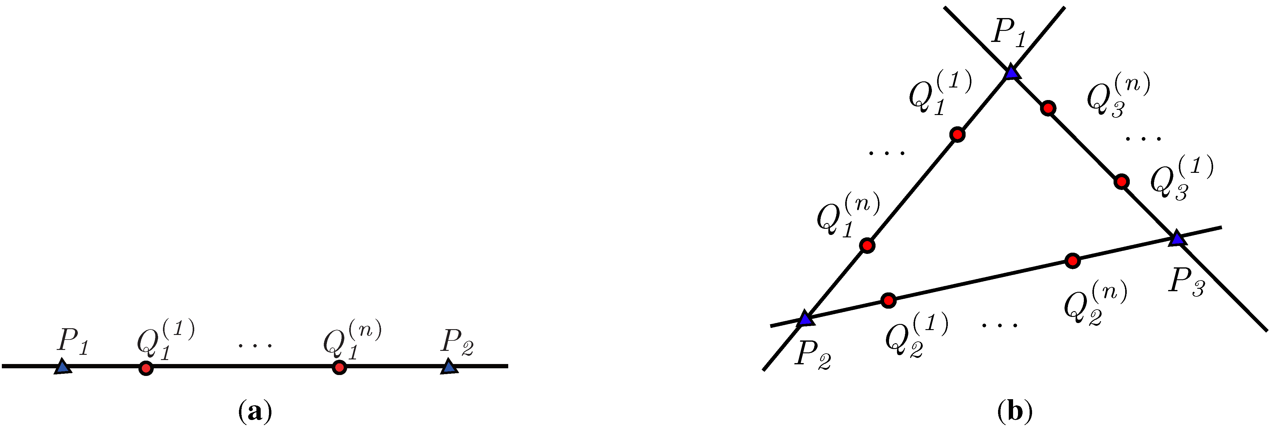
2.1. Characteristic Ratio: An Affine Invariant

Definition 1.

Let $p,q\in P^2$ be two different points (or lines) and $p_1,p_2,\cdots ,p_k$ be distinct points (or lines) on the line $(p,q)$, then there must exist $a_i$ and $b_i$, such that $p_i=a_{i}p+b_{i}q,(i=1,2,\cdots ,k)$. The ratio:

$$R(p_1,p_2,\cdots ,p_k):=\frac{b_1{b}_2\cdots b_k}{a_1{a}_2\cdots a_k}$$

(1)

is called the characteristic ratio (CR) of $p_1,p_2,\cdots ,p_k$ to the basic points (or basic lines), $p,q$.

The computation of CR is independent of the choice of the basic points. It is natural and straightforward to take x and y coordinates in the image plane as a and b, respectively. The mathematical aspects and significance of this ratio to algebraic curves can be found in our previous publication [19]. Herein, we provide the proof of its invariance to affine transformations, upon which we build our descriptors for 2D planar shapes.

Theorem 2.

The characteristic ratio given by Definition 1 is an affine invariant.

Proof.

The characteristic ratio can be calculated on any positive number of collinear points ($k\ge 1$). We first prove the case when $k=1$. Assuming three points, $x,y$ and v on a line, L, in the 3D world coordinate system, the points, $p,q,u$ and $p^{{}^{\prime }},q^{{}^{\prime }},u^{{}^{\prime }}$ are their images (as shown in Figure 1) obtained by two cameras with the optical centers, $O_1$ and $O_2$, respectively. It is well established that $p,q,u$ are collinear and so are $p^{{}^{\prime }},q^{{}^{\prime }},u^{{}^{\prime }}$. Any point in a line can be represented by the linear combination of other two points lying on the line, i.e.,

$$u=ap+bq,u^{{}^{\prime }}=a^{{}^{\prime }}{p}^{{}^{\prime }}+b^{{}^{\prime }}{q}^{{}^{\prime }}$$

(2)

for the lines of the two views in Figure 1, and thus, we need to prove $\frac{b}{a}=\frac{b^{{}^{\prime }}}{a^{{}^{\prime }}}$.

We assume that there exists an affine transformation between the images as the lines determined by the 2D points in both image planes are the images (projections) of the 3D line, L. The corresponding points in two views satisfy:

$$u^{{}^{\prime }}=Hu,p^{{}^{\prime }}=Hp,q^{{}^{\prime }}=Hq$$

(3)

Substituting Equation (3) into Equation (2), we have $Hu=a^{{}^{\prime }}Hp+b^{{}^{\prime }}Hq$. Since H is invertible, then we have:

$$u=a^{{}^{\prime }}p+b^{{}^{\prime }}q$$

(4)

Combining Equation (2) and Equation (4), we have $\frac{b}{a}=\frac{b^{{}^{\prime }}}{a^{{}^{\prime }a}}$, i.e., CR is an affine invariant when $k=1$.

Since every $\frac{b_k}{a_k}$ is affine invariant, CR with k multipliers of $\frac{b_k}{a_k}$ is an affine invariant when $k>1$. This establishes the theorem. ☐

Similar to the cross-ratio, the characteristic ratio reflects the geometric relationships of collinear points. Their difference lies in that the characteristic ratio has no limit on the number of the collinear points, while the cross-ratio defines on four collinear points. Hence, we are able to construct shape descriptors with more geometric information using the characteristic ratio on more points.

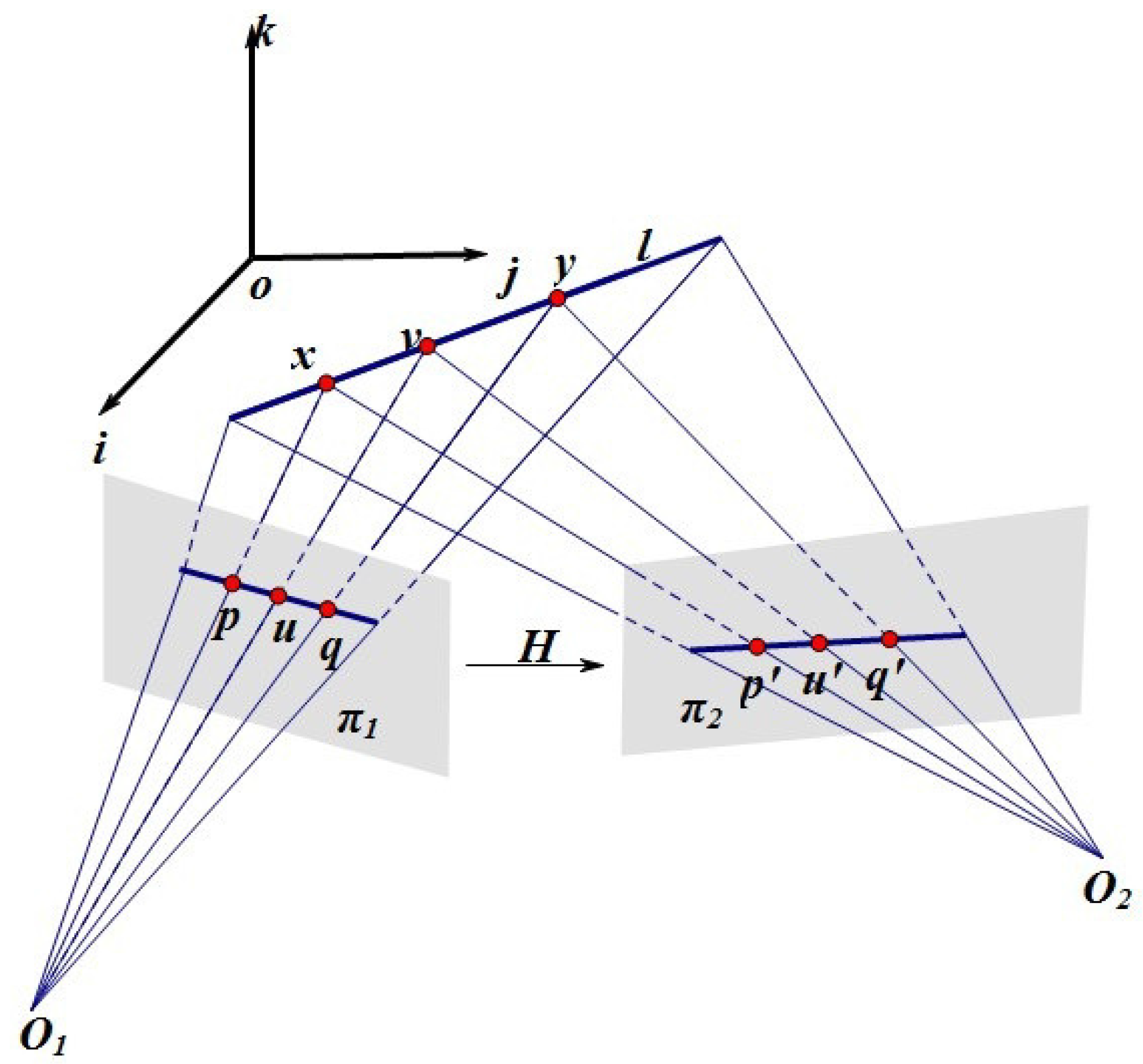
2.2. Characteristic Number: A Projective Invariant

The characteristic number can be regarded as a generalization of the cross-ratio, and we give the definition of the cross-ratio first. We adopt the convention that the upper symbol representing a point is also a column vector of the homogeneous coordinate for this point, and the lower ones are scalars. Let $P_1,P_2,P_3$ and $P_4$ be four collinear points and $P_1\ne P_4$. We have the linear representations of $P_2$ and $P_3$ as $a_1{P}_1+b_1{P}_4$ and $a_2{P}_4+b_2{P}_1$, respectively. The cross-ratio of these four points is:

$$(P_1{P}_2,P_3{P}_4):=\frac{a_1}{b_1}·\frac{a_2}{b_2}$$

(5)

We define the characteristic number as follows.

Definition 3.

Let $P_1,P_2,\dots ,P_{r-1},P_r$ be r distinct points in ${\mathbb{P}}^m\left(\mathbb{K}\right)$. On lines $P_i{P}_{i+1}$ forming a loop ($P_{r+1}:=P_1$ and $i=1,2,\dots ,r$), there are n points $Q_i^{\left(1\right)},Q_i^{\left(2\right)},\dots ,Q_i^{\left(n\right)}$ distinct from $P_i$ and $P_{i+1}$. Each $Q_i^{\left(j\right)}$ can be linearly represented by $P_i$ and $P_{i+1}$ as:

$$Q_i^{\left(j\right)}=a_i^{\left(j\right)}{P}_i+b_i^{\left(j\right)}{P}_{i+1}$$

Let $\mathcal{P}={\left\{P_i\right\}}_{i=1}^r$ and $\mathcal{Q}={\left\{Q_i^{\left(j\right)}\right\}}_{i=1,2,\dots ,r}^{j=1,2,\dots ,n}$, and define:

$${\kappa }_n(\mathcal{P},\mathcal{Q}):=\prod _{i=1}^r\prod _{j=1}^n\left(\frac{a_i^{\left(j\right)}}{b_i^{\left(j\right)}}\right)$$

(6)

as the characteristic number (of dimension m and degree n) of the point set, $\mathcal{Q}$, with respect to the frame point set, $\mathcal{P}$.

The following theorem shows that the invariance of CN to projective transformations.

Theorem 4.

The characteristic number is a projective invariant.

Proof:

Assume that a projective transform, Φ, projects $\mathcal{P}={\left\{P_i\right\}}_{i=1}^r$ to ${\mathcal{P}}^{{}^{\prime }}={\left\{P_i^{{}^{\prime }}\right\}}_{i=1}^r$, and we have $P_i{}^{\prime }=\Phi \left(P_i\right)=k_{i}H{P}_i(P_{r+1}=P_1,k_{i+1}=k_1)$. The points $\mathcal{Q}={\left\{Q_i^{\left(j\right)}\right\}}_{i=1,2,\dots ,r}^{j=1,2,\dots ,n}$ are projected to ${\mathcal{Q}}^{{}^{\prime }}={\left\{Q_i^{{\left(j\right)}^{\prime }}\right\}}_{i=1,2,\dots ,r}^{j=1,2,\dots ,n}$:

$$\begin{array}{cc}\hfill Q_i^{{\left(j\right)}^{\prime }}& =\Phi \left(Q_i^{\left(j\right)}\right)=l_i^{\left(j\right)}H{Q}_i^{\left(j\right)}=l_i^{\left(j\right)}H·(a_i^{\left(j\right)}{P}_i+b_i^{\left(j\right)}{P}_{i+1})\hfill \\ & =\frac{l_i^{\left(j\right)}{a}_i^{\left(j\right)}}{k_i}·k_{i}H{P}_i+\frac{l_i^{\left(j\right)}{b}_i^{\left(j\right)}}{k_{i+1}}·k_{i+1}H{P}_{i+1}\hfill \\ & =\frac{l_i^{\left(j\right)}{a}_i^{\left(j\right)}}{k_i}{P}_i^{{}^{\prime }}+\frac{l_i^{\left(j\right)}{b}_i^{\left(j\right)}}{k_{i+1}}{P}_{i+1}^{{}^{\prime }}\hfill \end{array}$$

Thus, the characteristic number of transformed points is given by:

$$\begin{array}{cc}\hfill {\kappa }_n({\mathcal{P}}^{{}^{\prime }},{\mathcal{Q}}^{{}^{\prime }})& =\prod _{i=1}^r\prod _{j=1}^n\left(\frac{k_{i+1}{l}_i^{\left(j\right)}{a}_i^{\left(j\right)}}{k_i{l}_i^{\left(j\right)}{b}_i^{\left(j\right)}}\right)\hfill \\ & =\prod _{i=1}^r\frac{k_{i+1}}{k_i}\left(\prod _{j=1}^n\frac{a_i^{\left(j\right)}}{b_i^{\left(j\right)}}\right)\hfill \\ & =\prod _{i=1}^r\left(\prod _{j=1}^n\frac{a_i^{\left(j\right)}}{b_i^{\left(j\right)}}\right)={\kappa }_n(\mathcal{P},\mathcal{Q})\hfill \end{array}$$

which indicates that the characteristic number is invariant under projective transformations. ☐

The characteristic number generalizes both the characteristic ratio and cross-ratio. The definition of CN in Equation (6) multiplies characteristic ratios, Equation (1), along a closed loop. Furthermore, the characteristic number of degree one of $Q_1^{\left(1\right)}$ and $Q_2^{\left(1\right)}$ with respect to the frame points, $P_1$ and $P_2$, degenerates to the cross-ratio, Equation (5), of $(P_1,P_2,Q_2^{\left(1\right)},Q_1^{\left(1\right)})$ when $r=2$ and $n=1$, as shown in Figure 2a. In other words, the cross-ratio is the simplified case ($n=1$) of the characteristic number in the two-dimensional space ($r=2$). This paper focuses on the applications of the characteristic number to 2D shape analysis, where the characteristic number can incorporate the geometric information on more points (i.e., $n\ge 1$) compared with the cross-ratio.

Figure 2. Points to calculate the characteristics number when (a) $r=2$ and (b) $r=3$.

Figure 2. Points to calculate the characteristics number when (a) $r=2$ and (b) $r=3$.

It is also worth noting that the numbers of points on any line segments between frame points are identical in the definition of CN. We give the two simplest cases for 2D shape analysis to calculate CN when $r=2$ and $r=3$. We consider two frame points, $P_1$ and $P_2$, when $r=2$. Let $Q_i^{\left(1\right)},Q_i^{\left(2\right)},\dots ,Q_i^{\left(n\right)}$ be n distinct points on the line segment, $P_1{P}_2$. For the case of even n, the odd-numbered points on the directed line, $P_1{P}_2$, and those even-numbered on $P_2{P}_1$ are used to compute CN:

$${\kappa }_n({\mathcal{P}}_2,{\mathcal{Q}}_2)=\prod _{i=1}^{\frac{n}{2}}\left(\frac{a_1^{(2i-1)}{b}_1^{\left(2i\right)}}{b_1^{(2i-1)}{a}_1^{\left(2i\right)}}\right)$$

(7)

where ${\mathcal{P}}_2=\{P_1,P_2\}$ and ${\mathcal{Q}}_2=\{Q_i^{\left(1\right)},Q_i^{\left(2\right)},\dots ,Q_i^{\left(n\right)}\}$. For odd n, we calculate CN in the same way by using all the points on the line segment, expect for the last one.

When $r=3$, let ${\mathcal{P}}_3=\{P_1,P_2,P_3\}$ and $Q_i^{\left(1\right)},Q_i^{\left(2\right)},\dots ,Q_i^{\left(n_i\right)}$ be $n_i$ distinct points on the edge $P_i{P}_{i+1}$ ($i=1,2,3$) of triangle, $▵P_1{P}_2{P}_3$, as illustrated in Figure 2b. We choose the closest $n=\min (n_1,n_2,n_3)$ points to $P_i$ on $P_i{P}_{i+1}$ as the set ${\mathcal{Q}}_3$ to calculate CN:

$${\kappa }_n({\mathcal{P}}_3,{\mathcal{Q}}_3)=\prod _{i=1}^3\prod _{j=1}^n\left(\frac{a_i^{\left(j\right)}}{b_i^{\left(j\right)}}\right)$$

(8)

2.3. Intrinsic Properties of a Hypersurface and Curve

In this section, we reveal an intrinsic geometric property of the points on an algebraic hypersurface or curve by using the characteristic number. This property is an extension of the well known Menelaus’s theorem and Carnot’s theorem in classical planar geometry and also a higher dimensional generalization of Serge [20] and Luo’s [18] results in a projective plane. Theorem 5 shows the intrinsic property of a hypersurface, and refer to [21] for the proof or the theorem that we omit here, due to the limitation of space.

Theorem 5.

Let $P_1,P_2,\dots ,P_{r-1},P_r$ be r distinct points in ${\mathbb{P}}^m\left(\mathbb{K}\right)$. On lines $P_i{P}_{i+1}$ ($P_{r+1}:=P_1$, and $i=1,2,\dots ,r$), there are n points $Q_i^{\left(1\right)},Q_i^{\left(2\right)},\dots ,Q_i^{\left(n\right)}$ distinct from $P_i$ and $P_{i+1}$. Some of these points may be the same. A hypersurface of degree n not through any $P_i$ intersects each line $P_i{P}_{i+1}$ precisely in ${\left\{Q_i^{\left(j\right)}\right\}}_{j=1}^n$ (multiple intersections are counted with multiplicities). Then, the characteristic number of ${\left\{Q_i^{\left(j\right)}\right\}}_{i=1,\dots ,r}^{j=1,\dots ,n}$ with respect to the frame points $P_1,P_2,\dots ,P_r$ is ${(-1)}^{rn}$. Conversely, if $P_1,\dots ,P_{m+1}$ are linearly independent and the characteristic number of ${\left\{Q_i^{\left(j\right)}\right\}}_{i=1,\dots ,r}^{j=1,\dots ,n}$ with respect to the frame points $P_1,P_2,\dots ,P_r$ is ${(-1)}^{(m+1)n}$, then all the $Q_i^{\left(j\right)}$ lie on a hypersurface of degree n not through any $P_i$.

Figure 3 shows an example of Theorem 5 in the three-dimensional Euclid space. Each $Q_i^{\left(j\right)}$ is distinct from the frame points, $P_i$, and then all ${\left\{Q_i^{\left(j\right)}\right\}}_{i=1,2,3,4}^{j=1,2}$ lie on a conic surface if and only if:

$${\kappa }_2({\left\{P_i\right\}}_{i=1}^4;{\left\{Q_i^{\left(j\right)}\right\}}_{i=1,2,3,4}^{j=1,2})=\prod _{i=1}^4\left(\frac{\left|P_{i+1}{Q}_i^{\left(1\right)}\right|}{\left|P_i{Q}_i^{\left(1\right)}\right|}·\frac{\left|P_{i+1}{Q}_i^{\left(2\right)}\right|}{\left|P_i{Q}_i^{\left(2\right)}\right|}\right)=1$$

where $\left|·\right|$ denotes the directed length.

Theorem 5 degenerates to the results of the characteristic number for algebraic curves partially presented in [18,19] if $m=2$ and $r=3$. These results reveal the intrinsic geometry of points on an algebraic curve that the characteristic number does not change with the selection of the base lines. As the simplest case in the two-dimensional space, the following corollary of Theorem 5, by setting $r=2$ and $n=1$, reflects the fundamental collinearity in the multi-view computer vision. Corollary 6 shows that the characteristic number ${\kappa }_1(P,Q,R)=-1$ in Figure 3b, regardless of the choice of base lines, $a,b$ and c, or points, $U,V$ and W. The value of CN for these three points also remains unchanged no matter from what viewpoint we capture the images, as shown in Figure 1. We can apply this property given by the characteristic number to matching collinear points on human faces with pose changes.

Corollary 6.

The characteristic number of three collinear points is −1.

Theorem 5 also shows that this property given by the characteristic number no longer depends on the existence of of an algebraic curve. Thereafter, we are able to calculate the characteristic number for points not necessarily lying on an algebraic curve as that in [18]. This calculation yields projective invariants on more points than five in the 2D space. In [4], Goodall and Mardia construct projective invariants on six points by combining cross-ratios and applying the invariant to object recognition problems involving collinear sets of points. Herein, we derive the characteristic number for any six coplanar points, as given in Corollary 7. We can also employ this invariant in order to match points on human faces along with the characteristic number for three points in Corollary 6.

Figure 3. Theorem 5 reveals the intrinsic properties of a hypersurface or curve. (a) An example for a surface in the three-dimensional Euclid space; (b) the characteristic number of three collinear points is $-1$; (c) the characteristic number on any six points derived from Theorem 5.

Figure 3. Theorem 5 reveals the intrinsic properties of a hypersurface or curve. (a) An example for a surface in the three-dimensional Euclid space; (b) the characteristic number of three collinear points is $-1$; (c) the characteristic number on any six points derived from Theorem 5.

Corollary 7.

Suppose that $A,B,C,H,I$ and J are six points, any three of which are not collinear on a projective plane, as shown in Figure 3c. The characteristic number, defined as the product of ratios of directed triangle areas below, is a projective invariant.

$$\kappa (A,I,C,H,B,J)=\frac{S_{▵ABH}}{S_{▵ACH}}.\frac{S_{▵BAI}}{S_{▵BCI}}.\frac{S_{▵CAJ}}{S_{▵CBJ}}$$

(9)

We can obtain the corollary by substituting $A,B,C$ as the frame points ${\mathcal{P}}_i$ and $D,E,F$ as the ${\mathcal{Q}}_i$ sets into Definition 3 and then applying Theorem 4. The areas in Equation (9) can be calculated by the determinants of the points’ homogenous coordinates:

$$\kappa =\frac{\left|ABH\right|}{\left|ACH\right|}.\frac{\left|BAI\right|}{\left|BCI\right|}.\frac{\left|CAJ\right|}{\left|CBJ\right|}$$

where:

$$\left|ABH\right|=\left|\begin{array}{ccc}1& 1& 1\\ x_a& x_b& x_h\\ y_a& y_b& y_h\end{array}\right|$$

The determinant operator is widely available in any programming packages for scientific computing.

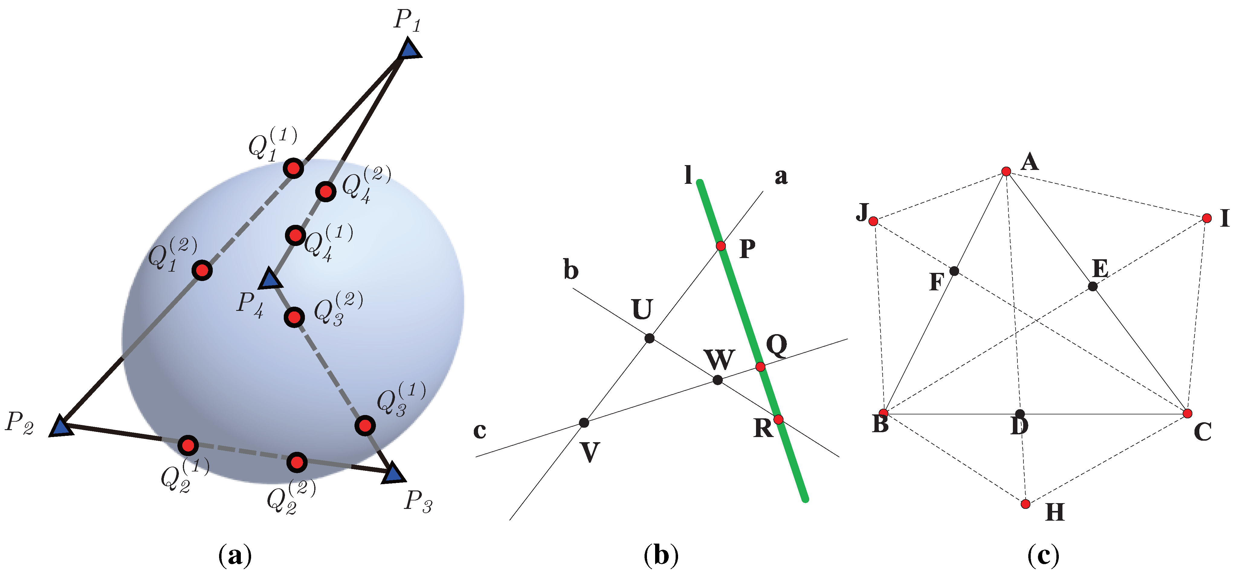
2.4. Generalization of Pascal’s Theorem

Classical Pascal’s theorem states the remarkable property of a hexagon inscribed in a conic. Various forms of generalizations emerge, but few of them appear in its original form. Luo et al. gave a generalization of Pascal’s theorem in the projective plane with a recursive structure in degrees, revealing the relation of curves of distinct degrees [18,19]. In this section, we present one generalization of Pascal’s theorem in a high-dimensional space.

Theorem 8.

Suppose $m,n\in {\mathbb{Z}}_{+}$ and $n\ge m$. $P_1,P_2,\dots ,P_{m+1}$ are $m+1$ linear independent points in ${\mathbb{P}}^m\left(\mathbb{K}\right)$. A hypersurface of degree n not through any $P_i$ intersects the lines $P_i{P}_{i+1}$ ($i=1,2,\dots ,m+1$ and $P_{m+2}:=P_1$) in the points $Q_i^{\left(1\right)},Q_i^{\left(2\right)},\dots ,Q_i^{\left(n\right)}$, where multiple intersections have distinct superscripts. For each $j(j=1,2,\dots ,m+1)$, the hyperplane, $H_j$, through ${\left\{Q_i^{\left(j\right)}\right\}}_{i\ne j}$ intersects the line $P_j{P}_{j+1}$ in $R_j$, and $S_j={\chi }_{(P_j,P_{j+1})}\left(R_j\right)$. Then, the $(m+1)(n-m+1)$ points ${\left\{S_j\right\}}_{j=1}^{m+1}\cup {\left\{Q_i^{\left(j\right)}\right\}}_{i=1,2,\dots ,m+1}^{j=i,m+2,m+3,\dots ,n}$ lie on a hypersurface of degree $n-m+1$ not through any $P_i$. (when $n=m$, we set $Q_i^{(m+1)}:=Q_i^{\left(i\right)}$ and ${\left\{Q_i^{\left(j\right)}\right\}}_{i=1,2,\dots ,m+1}^{j=i,m+2,m+3,\dots ,n}:=\varnothing$.)

This result establishes the connection from an algebraic hypersurface of higher degree to another one of lower degree as Pascal’s theorem and Luo’s results do to curves. Theorem 8 is equivalent to the results in [18,19] for planar curves when $m=2$. Furthermore, this theorem degenerates to Pascal’s theorem if the hypersurface (algebraic curve) is a conic. The proof of the theorem is given in [21], rather, due to the limit of the space, and we will provide its applications in future work.

3. Application I: A Perspective Invariant Shape Descriptor

We have used the characteristic ratio in Definition 1 to construct a shape descriptor invariant to affine transformations, named the characteristic ratio spectrum (CHARS) [22]. Compared with the descriptor using the cross-ratio (CRS) [7], our descriptor is able to incorporate more shape information, especially on geometric structures inside the symbol, as the cross-ratio in CRS can only use four collinear points for the calculation, but the characteristic ratio can combine as many as available. As shown in Figure 4d,e, most circles are left by the calculation of the cross-ratio. The loss of the information inside the symbol results in that CRS in Figure 4b cannot discriminate the symbols with subtle inner differences, as shown in Figure 4a. In contrast to the cross-ratio, the new characteristic ratio is able to make use of all available edge points given by the circles in Figure 4d,e and, thus, yields the spectra in Figure 4c showing the differences for the symbols. Refer to [22] for more details on descriptor construction and experimental comparisons on symbol recognition.

Similarly, we are able to construct a shape descriptor invariant to perspective deformations [8] using the characteristic number defined as Definition 3, which is expected to incorporate more information on the inner structures.

Figure 4. Comparison between characteristic ratio spectrum (CHARS) and cross-ratio spectrum (CRS). (a) Two symbols with subtle inner differences; (b) The cross-ratio spectra of the symbols; (c) The characteristic ratio spectra of the symbols; (d) and (e) illustrate the inner points used to calculate CHARS (circles) and CRS (red dots) of the symbols.

Figure 4. Comparison between characteristic ratio spectrum (CHARS) and cross-ratio spectrum (CRS). (a) Two symbols with subtle inner differences; (b) The cross-ratio spectra of the symbols; (c) The characteristic ratio spectra of the symbols; (d) and (e) illustrate the inner points used to calculate CHARS (circles) and CRS (red dots) of the symbols.

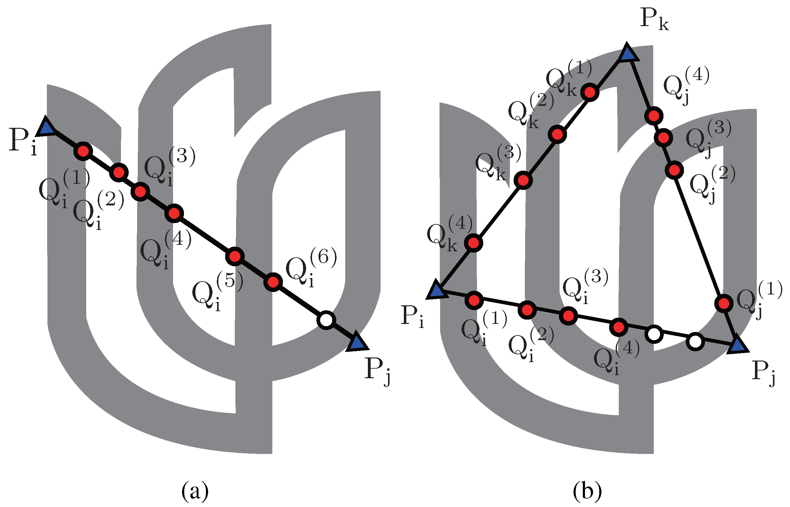
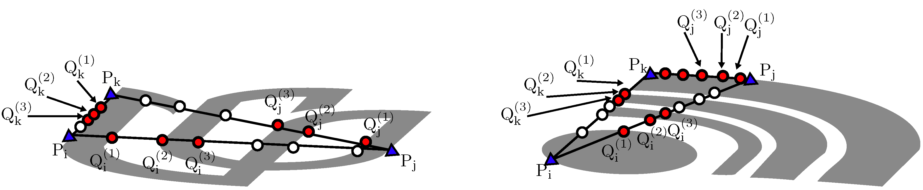
3.1. Descriptor Construction

Similar to CRS and CHARS, we concatenate the values of invariants, the characteristic number here, to form the descriptor. As shown in Definition 3, we have to construct the closed loops to calculate CN. Let $\mathcal{P}=\left\{P_s\}\right(s=1,2,\dots ,N)$ denote the equidistant sample points numbered counter-clockwise on the convex hull of a given shape, $\mathcal{S}$. We pick out three points in turn from $P_s$ as $P_i,P_j,P_k$ $(i=1,2,\dots ,N-2,j=i+1,i+2,\dots ,N-1,k=j+1,j+2,\dots ,N)$. The characteristic number $\kappa (P_i,P_j,P_k)=-1$, if they are collinear. Otherwise, these three points form a triangle, and there are $C_N^3$ triangles in total that cover the whole shape. As shown in Figure 5, each side of the triangle intersects the inner shape at several points regarded as $Q_i$ for the calculation of CN. We can obtain $\kappa (P_i,P_j,P_k)$ of the triangle $▵P_i{P}_j{P}_k$ by Equation (8). We concatenate the CN values of the triangles as the descriptor for the shape, $\mathcal{S}$:

$${\mathcal{D}}_1\left(\mathcal{S}\right)=\left(\kappa (P_i,P_j,P_k)\right)$$

(10)

where $i=1,2,\dots ,N-2,j=i+1,i+2,\dots ,N-1,k=j+1,j+2,\dots ,N$. ${\mathcal{D}}_1\left(\mathcal{S}\right)$ is a vector of length $C_N^3$.

Figure 5. Points to calculate the characteristic number when (a) $r=2$ and (b) $r=3$.

Figure 5. Points to calculate the characteristic number when (a) $r=2$ and (b) $r=3$.

In practical applications, one side of a triangle may have coincidence with the convex hull. False intersections are detected and used $N-2$ times in this case. These intersections cannot reflect the inner structure of the shape correctly and, hence, introduce errors in shape matching. We discard the intersections whose distances to the convex hull are smaller than a given threshold.

Another practical issue arises when any sides of $▵P_i{P}_j{P}_k$ do not intersect the shape, $\mathcal{S}$. The shape geometries are not available in the descriptor if we simply set $\kappa (P_i,P_j,P_k)$ to zero in this case, no matter how many intersections exist on the other sides. To address this issue, we define $\kappa (P_i,P_j,P_k)$ as follows assuming that the segment, $P_k{P}_i$, dose not intersect the shape without loss of generality.

• $\kappa (P_i,P_j,P_k)=\kappa (P_i,P_j)·\kappa (P_j,P_k)$ if there are at least two intersections on both sides, $P_i{P}_j$ and $P_j{P}_k$.
• $\kappa (P_i,P_j,P_k)=\kappa (P_j,P_k)$(or $\kappa (P_i,P_j)$) if there are at least two intersections on the side, $P_j{P}_k$ (or $P_i{P}_j$), and no more than one intersection on the side, $P_i{P}_j$ (or $P_j{P}_k$).
• $\kappa (P_i,P_j,P_k)=0$ if there is at most one intersection on either $P_i{P}_j$ or $P_j{P}_k$.

Theoretically, the descriptor for one shape remains unchanged under projective transformations. Unfortunately, we may detect false intersections, due to significant deformations that do not preserve parallelism. In the following, we justify the applicability of the descriptor to complex shapes under perspective transformations by its properties.

• The characteristic number on a triangle is permutable, i.e., $\kappa (P_i,P_j,P_k)=\kappa (P_j,P_k,P_i)=\kappa (P_k,P_i,$$P_j)$. This can be be readily verified by Equation (8).
• The choice of initial point (triangle) does not change individual values in $\mathcal{D}\left(\mathcal{S}\right)$, but determines the order in which CN values appear in $\mathcal{D}\left(\mathcal{S}\right)$. It is also straightforward to derive this property from the above and Equation (10).
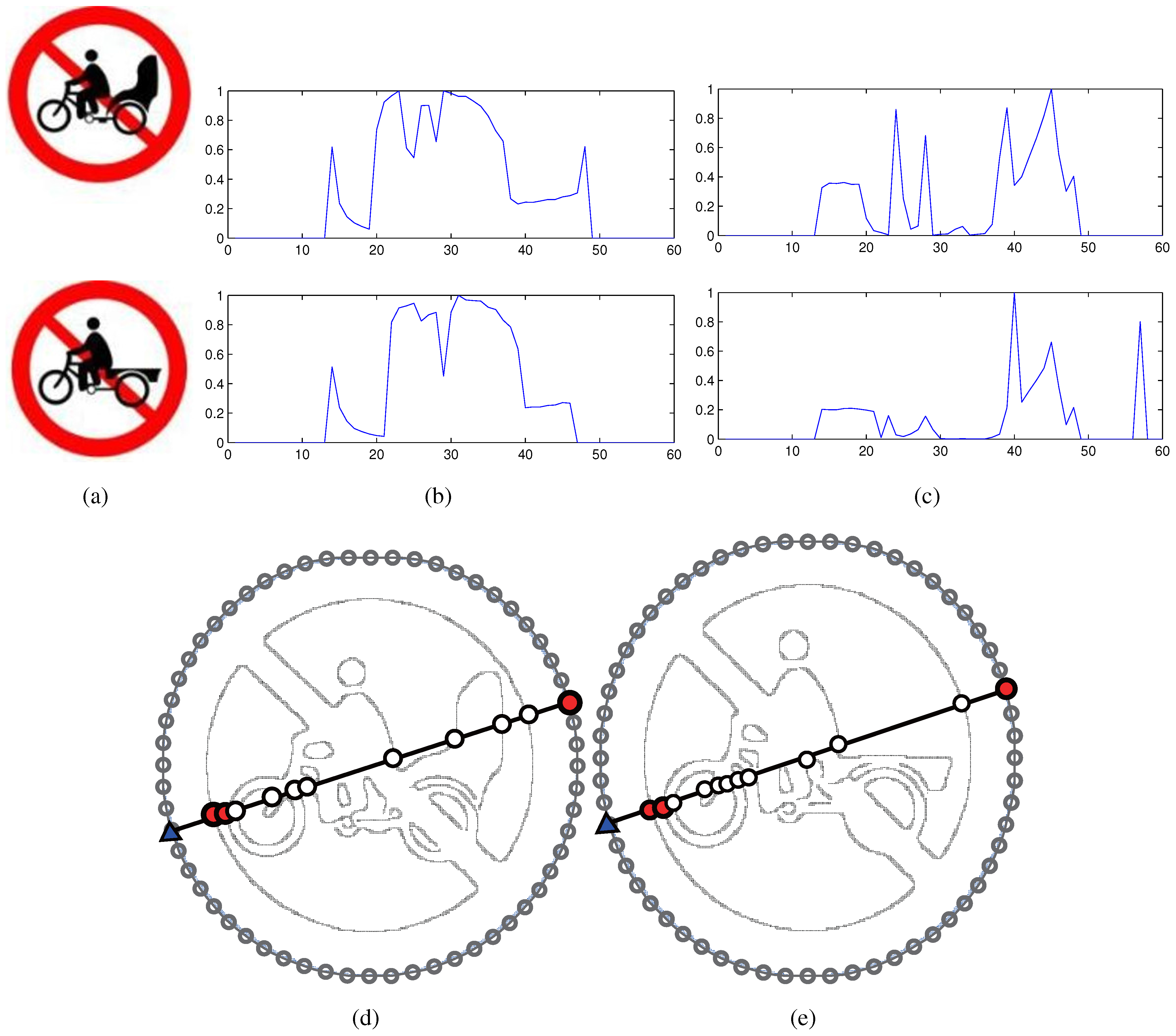
• Slight fluctuations of the vertices on the convex hull of $\mathcal{S}$ bring gradual changes on $\mathcal{D}\left(\mathcal{S}\right)$. It is assumed that three pairs of points, ($P_i$, $P_i^{\prime }$), ($P_j$, $P_j^{\prime }$) and ($P_k$, $P_k^{\prime }$), are neighbors on the smooth part of convex hull. We have $\kappa (P_i,P_j,P_k)\approx \kappa (P_i^{\prime },P_j^{\prime },P_k^{\prime })$, since each side of the triangles to calculate CN values is also close to each other.
• The descriptor presents fluctuations in the case of affine transformations due to jags on the inner intersections. Severe perspective deformations would make it worse. A dynamic programming algorithm, i.e., dynamic time warping (DTW), is employed to align the shape descriptors of query and template shapes, as done in CRS and CHARS. This process can alleviate the deviations brought by the choice of the starting point.

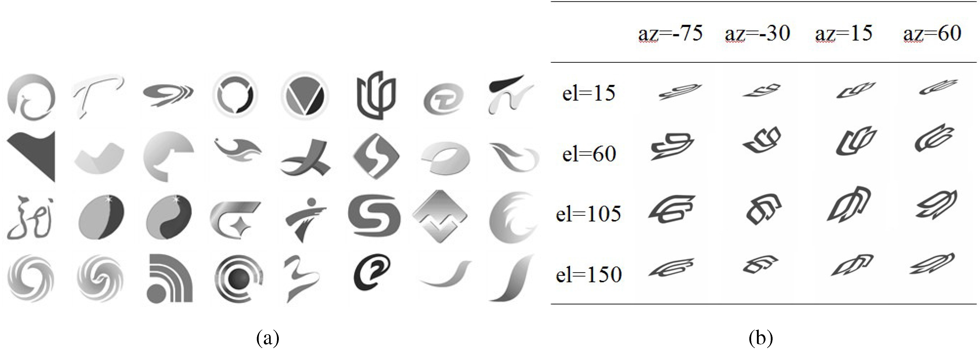
3.2. Performance Evaluation

We evaluate the performance of the descriptor (CNF) derived from CN by comparing with recent CRS [7] and SIFT [23], the most successful feature descriptor so far. All experiments are conducted on a PC with a 2.3 GHz CPU and 4 GB memory. We follow exactly the same similarity metrics for descriptors and the DTW alignment process as CRS and CHARS in all our experiments.

We validate the proposed descriptor on 32 logos of television networks among which, similar shapes exist, as shown in Figure 6. Furthermore, many logos appear as relatively complex shape structures, especially within their convex hulls. The query sets are generated by changing the azimuth (az) and elevation (el) angles, as well as two factors $(\alpha ,\beta )$ to indicate the degree of perspective deformations. The larger $(\alpha ,\beta )$ are, the more severe is the perspective deformation. We have three degrees of deformations, i.e., $(\alpha ,\beta )$ are $(0.5,0)$, $(1.0,0.5)$ and $(1.5,0.5)$, and generate 16 types of (az, el) combinations for each degree. We generate binary contours by simply applying the Canny edge detector available in the MATLAB Image Processing toolbox. No extra smoothing or parameterization [24] is included.

Figure 6. Experimental set: (a) 32 logos of television networks; and (b) an example subject to perspective transformations with the perspective factors $(\alpha ,\beta )=(0.5,0)$ and various ($az$, $el$) (azimuth (az) and elevation (el)) parameters.

Figure 6. Experimental set: (a) 32 logos of television networks; and (b) an example subject to perspective transformations with the perspective factors $(\alpha ,\beta )=(0.5,0)$ and various ($az$, $el$) (azimuth (az) and elevation (el)) parameters.

Table 1, Table 2 and Table 3 show the recognition rates given by the descriptors (CNF) from the characteristic number compared with CRS and SIFT under perspective deformations. It can be seen that CNF has a better performance than the other two methods in most projective transformations. CNF yields very high recognition rates when $el=60$ and 105 no matter what $(\alpha ,\beta )$ is. When $(\alpha ,\beta )=(0.5,0)$, CNF shows superior performance on 13 out of 16 query subsets. The performance of CNF degrades as as $(\alpha ,\beta )$ increases, but there are still 11 and 10 out of 16 query subsets showing higher rates when $(\alpha ,\beta )=(1.0,0.5)$ and $(\alpha ,\beta )=(1.5,0.5)$, respectively. CNF is also a bit worse than CRS when the perspective deformations become significantly severe. In these cases, the triangle sides that generate our descriptor have significant coincidence with the convex hull, so that inaccurate intersections are detected, as shown in Figure 7. A simple threshold cannot eliminate all these inaccurate intersections that bring more side effects to our descriptor, as ours include more points than CRS does.

Table 1. Recognition rates on the query set when $\alpha =0.5$ and $\beta =0$. CNF, descriptor derived from the characteristic number; CRS, cross-ratio spectrum.

	CNF				CRS				SIFT
az	$-{75}^{°}$	$-{30}^{°}$	${15}^{°}$	${60}^{°}$	$-{75}^{°}$	$-{30}^{°}$	${15}^{°}$	${60}^{°}$	$-{75}^{°}$	$-{30}^{°}$	${15}^{°}$	${60}^{°}$
$el={15}^{°}$	43.75	50	50	59.38	50	62.5	46.88	46.88	6.25	9.38	6.25	15.63
$el={60}^{°}$	93.75	100	96.88	96.88	87.5	84.38	87.5	87.5	28.13	65.63	53.13	25
$el={105}^{°}$	100	100	100	100	93.75	90.63	90.63	87.5	12.5	71.88	71.88	21.88
$el={150}^{°}$	71.88	75	87.5	75	68.75	84.38	84.38	68.75	6.25	18.75	25	3.13

Table 1. Recognition rates on the query set when $\alpha =0.5$ and $\beta =0$. CNF, descriptor derived from the characteristic number; CRS, cross-ratio spectrum.

	CNF				CRS				SIFT
az	$-{75}^{°}$	$-{30}^{°}$	${15}^{°}$	${60}^{°}$	$-{75}^{°}$	$-{30}^{°}$	${15}^{°}$	${60}^{°}$	$-{75}^{°}$	$-{30}^{°}$	${15}^{°}$	${60}^{°}$
$el={15}^{°}$	43.75	50	50	59.38	50	62.5	46.88	46.88	6.25	9.38	6.25	15.63
$el={60}^{°}$	93.75	100	96.88	96.88	87.5	84.38	87.5	87.5	28.13	65.63	53.13	25
$el={105}^{°}$	100	100	100	100	93.75	90.63	90.63	87.5	12.5	71.88	71.88	21.88
$el={150}^{°}$	71.88	75	87.5	75	68.75	84.38	84.38	68.75	6.25	18.75	25	3.13

Table 2. Recognition rates on the query set when $\alpha =1.0$ and $\beta =0.5.$

	CNF				CRS				SIFT
az	$-{75}^{°}$	$-{30}^{°}$	${15}^{°}$	${60}^{°}$	$-{75}^{°}$	$-{30}^{°}$	${15}^{°}$	${60}^{°}$	$-{75}^{°}$	$-{30}^{°}$	${15}^{°}$	${60}^{°}$
$el={15}^{°}$	37.5	62.5	43.75	50	53.13	53.13	34.38	34.38	6.25	6.25	0	6.25
$el={60}^{°}$	90.63	100	100	78.13	84.38	84.38	81.25	75	12.5	31.25	25	9.38
$el={105}^{°}$	96.88	100	93.75	87.5	87.5	90.63	87.5	71.88	18.75	46.88	40.63	9.38
$el={150}^{°}$	56.25	75	62.5	53.13	75	78.13	65.63	65.63	12.5	12.5	12.5	15.63

Table 2. Recognition rates on the query set when $\alpha =1.0$ and $\beta =0.5.$

	CNF				CRS				SIFT
az	$-{75}^{°}$	$-{30}^{°}$	${15}^{°}$	${60}^{°}$	$-{75}^{°}$	$-{30}^{°}$	${15}^{°}$	${60}^{°}$	$-{75}^{°}$	$-{30}^{°}$	${15}^{°}$	${60}^{°}$
$el={15}^{°}$	37.5	62.5	43.75	50	53.13	53.13	34.38	34.38	6.25	6.25	0	6.25
$el={60}^{°}$	90.63	100	100	78.13	84.38	84.38	81.25	75	12.5	31.25	25	9.38
$el={105}^{°}$	96.88	100	93.75	87.5	87.5	90.63	87.5	71.88	18.75	46.88	40.63	9.38
$el={150}^{°}$	56.25	75	62.5	53.13	75	78.13	65.63	65.63	12.5	12.5	12.5	15.63

Table 3. Recognition rates on the query set when $\alpha =1.5$ and $\beta =0.5.$

	CNF				CRS				SIFT
az	$-{75}^{°}$	$-{30}^{°}$	${15}^{°}$	${60}^{°}$	$-{75}^{°}$	$-{30}^{°}$	${15}^{°}$	${60}^{°}$	$-{75}^{°}$	$-{30}^{°}$	${15}^{°}$	${60}^{°}$
$el={15}^{°}$	31.25	31.25	37.5	31.25	40.63	50	34.38	21.88	6.25	9.38	6.25	15.63
$el={60}^{°}$	87.5	84.38	84.38	62.5	87.5	78.13	78.13	59.38	28.13	65.63	53.13	25
$el={105}^{°}$	87.5	93.75	90.63	75	78.13	87.5	81.25	71.88	12.5	68.75	68.75	21.88
$el={150}^{°}$	43.75	62.5	53.13	46.88	65.13	68.75	62.5	56.25	6.25	18.75	25	3.13

Table 3. Recognition rates on the query set when $\alpha =1.5$ and $\beta =0.5.$

	CNF				CRS				SIFT
az	$-{75}^{°}$	$-{30}^{°}$	${15}^{°}$	${60}^{°}$	$-{75}^{°}$	$-{30}^{°}$	${15}^{°}$	${60}^{°}$	$-{75}^{°}$	$-{30}^{°}$	${15}^{°}$	${60}^{°}$
$el={15}^{°}$	31.25	31.25	37.5	31.25	40.63	50	34.38	21.88	6.25	9.38	6.25	15.63
$el={60}^{°}$	87.5	84.38	84.38	62.5	87.5	78.13	78.13	59.38	28.13	65.63	53.13	25
$el={105}^{°}$	87.5	93.75	90.63	75	78.13	87.5	81.25	71.88	12.5	68.75	68.75	21.88
$el={150}^{°}$	43.75	62.5	53.13	46.88	65.13	68.75	62.5	56.25	6.25	18.75	25	3.13

Figure 7. Significantly severe deformations bring inaccurate points into the new descriptor.

Figure 7. Significantly severe deformations bring inaccurate points into the new descriptor.

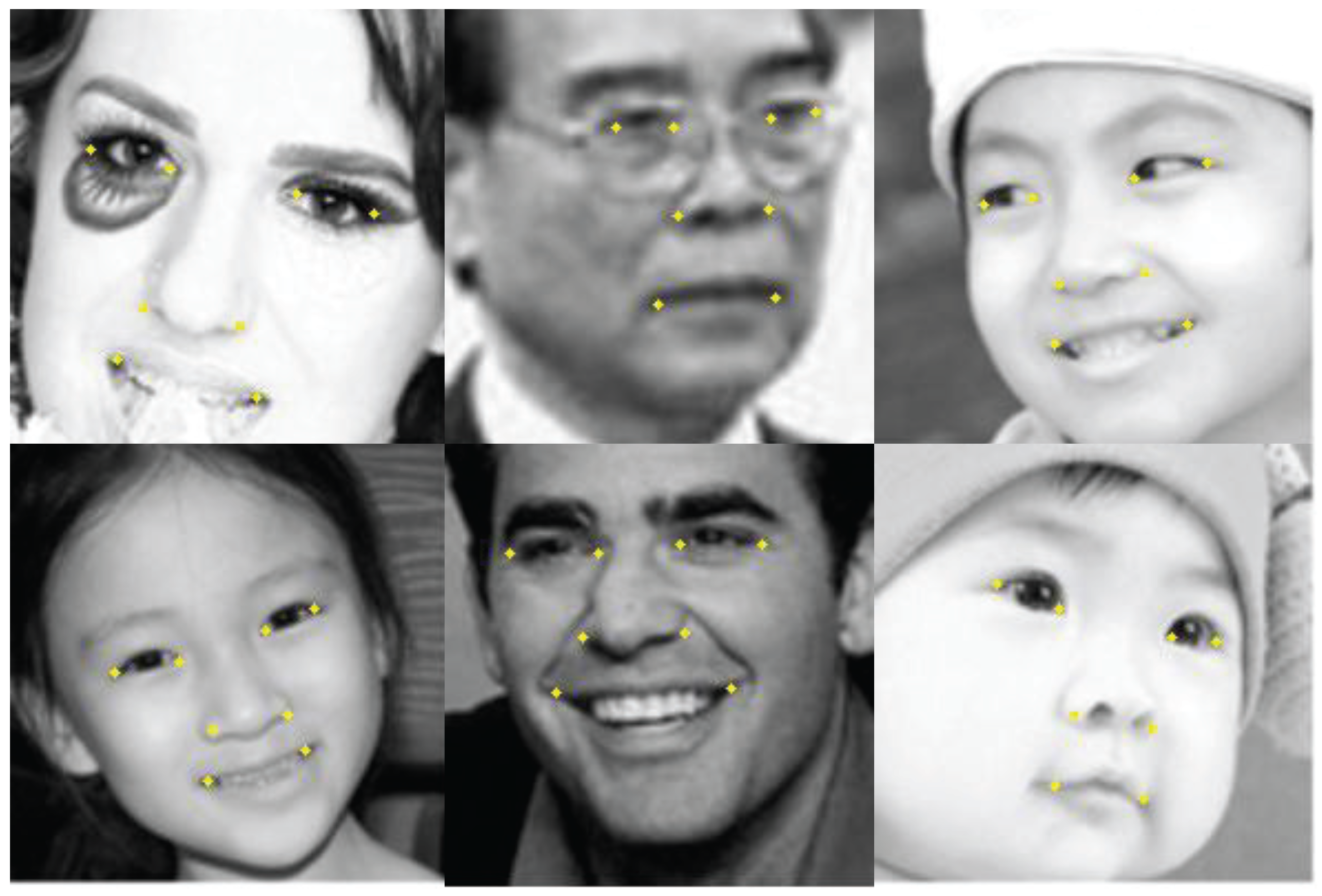
4. Application III: Shape Matching with Characteristic Number

The characteristic number reflects the intrinsic properties of the algebraic curve given by several points, and these properties do not rely on the existence of the curve, as shown in Section 2.3. We are able to discover these properties through the characteristic number that is invariant to projective transformations and apply them as geometric constraints to the extraction of facial feature points under viewpoint or pose changes. The extraction problem is typically formulated as matching an appearance model with facial shape constraints. In this section, we use the local appearance model based on the principal component analysis (PCA) in [25,26] and substitute their PCA-based shape constraints with our facial priors discovered by the characteristic number. Our priors derived from CN are invariant to projective/perspective transformations and, hence, render the robustness to viewpoint or pose changes to the extraction algorithm.

4.1. Shape Priors Using Characteristic Number

Human faces are highly structured and present common geometries across the age, gender and ethnicity of individuals. For example, the four eye corners are collinear, and this collinearity preserves under pose/viewpoint changes. Researchers employ this invariant property of collinearity for pose recovery [27]. We intend to incorporate more geometric constraints than the collinearity.

The CN invariant is able to characterize more geometric information on faces in addition to the collinearity. We take an exhausted strategy on the CN values for the subsets of fiducial points in order to discover their common geometries. We enumerate all possible combinations of choosing three, five and six points from eight manually labeled fiducial points and calculate the CN value on every combination for all 515 images. Taking the discovery process of the collinearity using CN as an example, we have $C_8^3=56$ three-point combinations. Each combination generates 515 CN values for 515 frontal faces. Corollary 6 tells us that the CN value of three collinear points is a constant $-1$, so that we can pick out four combinations with three collinear points satisfying:

$$|(-1)-C{N}_{sub}{|}^2<\epsilon$$

(11)

where $C{N}_{sub}$ is the CN of the three-point subsets and ε is a small positive constant. The blue bar in Figure 8a shows the histogram of the CN values for one three-point combination that satisfies Equation (11) on 515 frontal faces. Almost all the CN values of the points, whose locations are annotated as blue dots on the top frontal face in Figure 8b, are quite close to $-1$. We verify the invariance of the prior by using the same three-point combination from the other set of 515 uncontrolled faces with different poses and identities, one of which is given in the top image of Figure 8d. The CN values calculated from all these points are almost equal to $-1$, as we expect. These histograms verify that CN can find the collinear fiducial points on human faces, and the collinearity remains.

We perform the similar screening process on the combinations of five and six points, whose CN values are approximately identical for all 515 frontal faces:

$$\left\{\begin{array}{c}\hfill |C-C{N}_{sub}{|}^2<\epsilon \\ \hfill Sd\left(C{N}_{sub}\right)<\sigma \end{array}\right.$$

(12)

where $Sd(·)$ denotes the standard deviation and σ is a small positive constant. The constant, C, is called the intrinsic value that characterizes the geometric property of the curve underlying six points. We find six combinations for five-point and six for six-point subsets that follow Equation (12). The histograms and point locations on frontal faces are given in Figure 8a,b, respectively. The CN values of one combination for all 515 frontal faces concentrate on one definite value. Again, Figure 8c,d verifies the projective invariances of CN on five (cross-ratio) and six points given by Corollary 7. These invariant priors, reported for the first time to the best of our knowledge, reflect common facial geometries similar to the collinearity, but on a larger scale, involving more points for more facial components. We can calculate these priors, as well as the collinearity with one formula, as Equation (6).

Figure 8. CN values for subsets with three (blue), five (red) and six (green) points: (a) histograms of CN values on the subsets of fiducial points whose locations are annotated in the frontal face images in (b), and (c) histograms of CN values on the same combinations of points as (a). The point coordinates for (c) are extracted from images in (d), significantly different from (b). Horizontal axes of the histograms are CN values, and the vertical axes are the number of faces.

Figure 8. CN values for subsets with three (blue), five (red) and six (green) points: (a) histograms of CN values on the subsets of fiducial points whose locations are annotated in the frontal face images in (b), and (c) histograms of CN values on the same combinations of points as (a). The point coordinates for (c) are extracted from images in (d), significantly different from (b). Horizontal axes of the histograms are CN values, and the vertical axes are the number of faces.

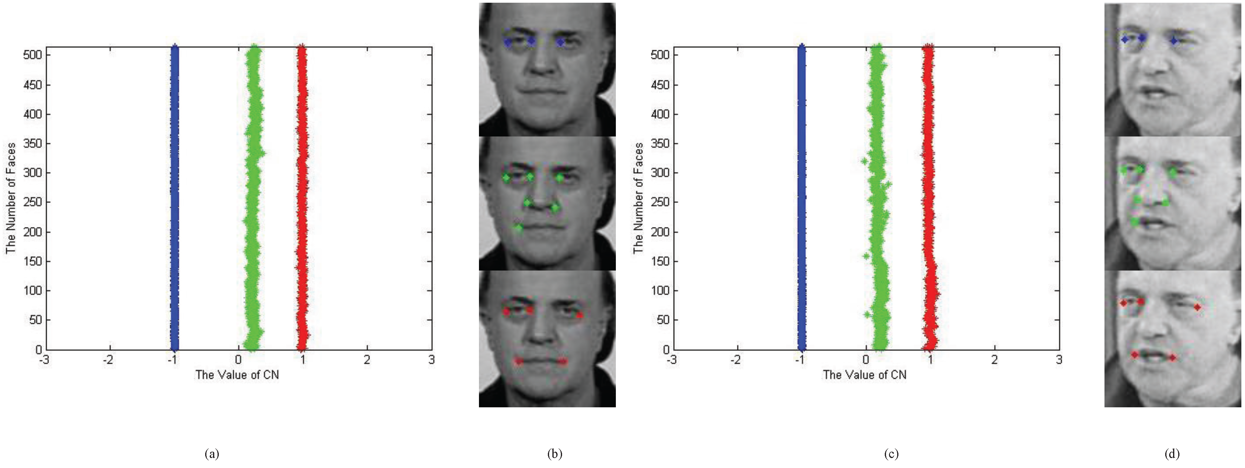
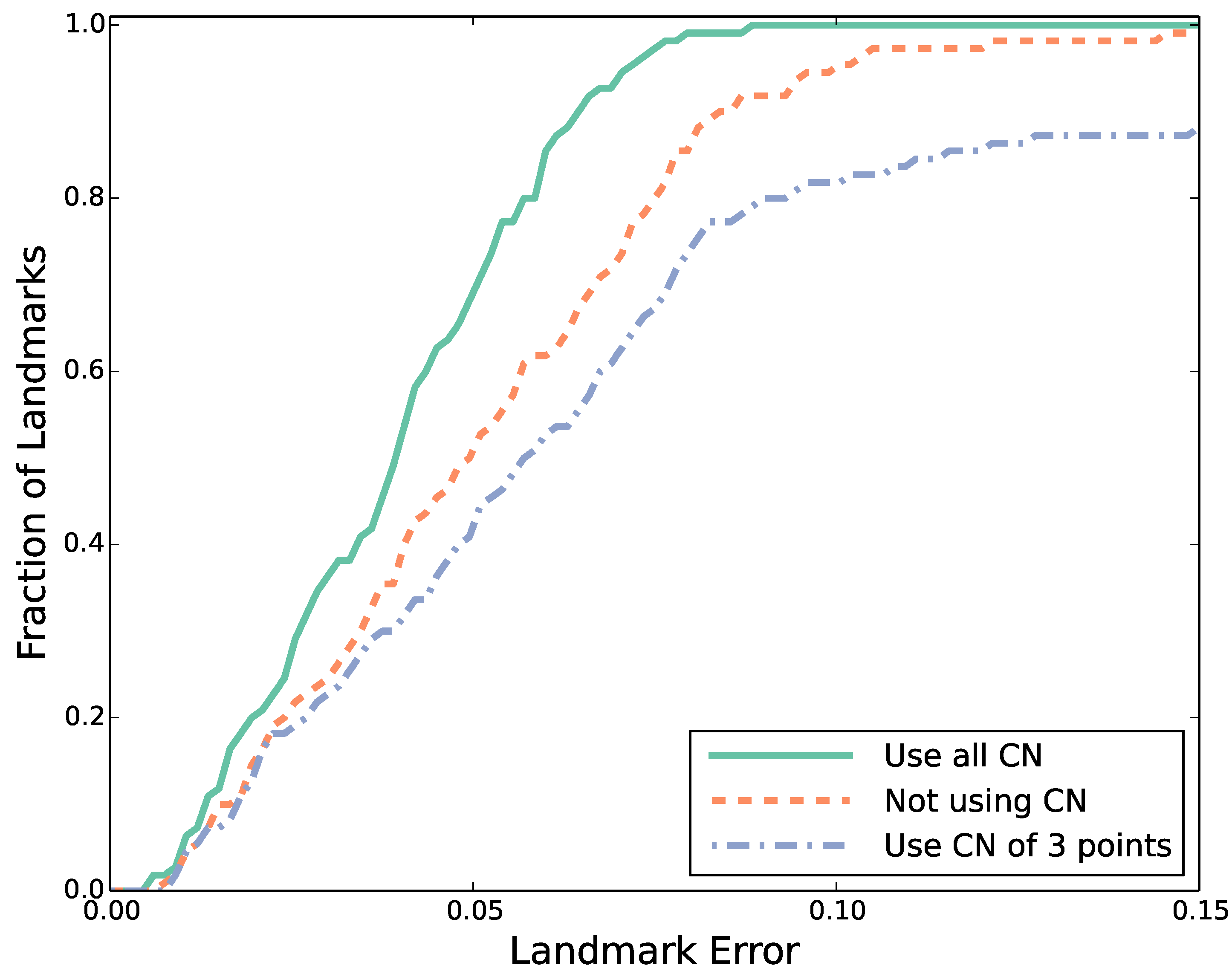
4.2. Performance Evaluation

We use the Viola–Jones face detector [28] available at OpenCV to pick out the faces with both the eyes, nose and mouth presented. The detector can also output the regions of eyes and mouth for each detected face. We use these regions to roughly initialize the positions of eight fiducial points. The shape priors derived from CN are used as the constraints to match PCA-based appearance models on local patches around the fiducial points and, finally, localize these points.

We test our algorithm on facial images with a wide range of variations on poses, expressions and ages from a commercial set and several public face sets, including IMM-FACE-DB [29], LFW [30], AFLW [31] and Pointing’04 [32]. IMM-FACE-DB and Pointing’04 are the sets of medium scale under controlled environment, which categorizes facial images into identities and types of variations. LFW and AFLW have more than $10,000$ facial images in the wild, and the commercial set complement the testing images with faces of young children. We randomly select 500 images from these sets of different environments for quantitative comparisons with the approach without and with partial shape constraints in order to demonstrate the generalization of the CN-based shape priors.

Figure 9. Fiducial point localization with pose changes, as well as variations on age, expression and resolution.

Figure 9. Fiducial point localization with pose changes, as well as variations on age, expression and resolution.

We employ the normalized mean error (NME) as the objective metric for qualitative comparisons. This metric is widely accepted in comparative studies for facial point localization and alignment and is defined as:

$$m_e=\frac{1}{n{d}_{lr}}\sum _{i=1}^n{d}_i$$

(13)

where n denotes the number of landmarks and $d_i$ values are the Euclidean point-to-point distances between the estimated locations and manually labeled ground-truth. The distance, $d_i$, is normalized by $n{d}_{lr}$, the distance between two pupils for each face.

Figure 9 shows the selected results of our algorithm on the testing images. Our algorithm works well on faces with pose and expression changes. The used shape constraints of the algorithm can help recover the accurate positions when glasses or partial occlusions appear in the facial images in Figure 9. The algorithm is also insensitive to low resolutions (LR), as long as the face detector can find a face from the LR image. The local facial appearance may change, but the global facial geometry preserves when a person is growing. Our CN-based shape priors, especially those on five and six points, can reflect the geometry at a larger scale and, thus, is applicable to images of babies and toddlers, though we discover the priors from adult faces. Figure 9 also demonstrates the accurate and robust localization of our algorithm on children images.

We show the impacts of the CN-based shape priors by comparing the localization accuracies when using collinearity (CN on three points), all CN constraints and no shape constraints. We calculate NMEs on 110 testing images selected from the data sets referred to above and plot the cumulative error distributions [33,34] of the three configurations in Figure 10. We can hardly reduce the errors lower than 0.15 for nearly 15% images if no geometric constraint is imposed on our optimization framework. The introduction of collinearity improves the accuracy of eye corner localization, so that the errors are down to about 0.12 for almost all images. More significantly, the errors are less than 0.1 for all the images when we combine more shape constraints derived from CN on five and six points. These improvements validate the use of our CN-based shape priors.

Figure 10. Cumulative error distributions of localizations with collinearity (three-point CN, red dots), all CN constraints (green solid and no shape constraints (blue dash dots). The x-axis is the normalized mean error (NME), and the y-axis indicates the percentage of images on which localization NMEs are lower than the x-value.

Figure 10. Cumulative error distributions of localizations with collinearity (three-point CN, red dots), all CN constraints (green solid and no shape constraints (blue dash dots). The x-axis is the normalized mean error (NME), and the y-axis indicates the percentage of images on which localization NMEs are lower than the x-value.

5. Conclusions

In this paper, we present a projective invariant, named the characteristic number, defined on looped line segments. This invariant does not rely on the existence of the underlying algebraic surface or curves as its planar version in [18,19]. Compared with the classical cross-ratio, the invariant is able to include more non-collinear points, which paves the way for the possibilities of more informative descriptors and constraints. The computation of the characteristic number only involves simple multiplications and divisions of the point coordinates, as shown in Equation (6), and its complexity is linear to the number of points in the set, $\mathcal{Q}$. We demonstrate the potentials of the invariant on the applications of shape recognition and matching under affine and perspective transformations. The new definition of the characteristic number also applies in a higher dimensional space.

The characteristic number defined in Equation (6) requires that the point numbers of the sets, $\mathcal{Q}$, between any two frame points should be identical. Currently, we have to trim some inner points on one or several segments between frame points in order to meet the requirement as discussed in Section 3. This treatment is simple, but may sacrifice the descriptive ability. We are developing new invariants that relax this constraint. Furthermore, our invariant is applicable in a higher dimensional space, and hence, we will investigate how the invariant works for 3D shape analysis in the future.

References

1. Hartley, R.; Zisserman, A. Multiple View Geometry in Computer Vision, 2nd ed.; Cambridge University Press: Cambridge, UK, 2004. [Google Scholar]
2. Weiss, I. Geometric invariants and object recognition. Int. J. Comput. Vis. 1993, 10, 207–231. [Google Scholar] [CrossRef]
3. Lin, W.Y. Robust Geometrically Invariant Features for 2D Shape Matching and 3D Face Recognition. Ph.D. Thesis, University of Wisconsin-Madson, Madison, WI, USA, 2006. [Google Scholar]
4. Goodall, C.R.; Mardia, K.V. Projective shape analysis. J. Comput. Graph. Stat. 1999, 8, 143–168. [Google Scholar]
5. Suk, T.; Flusser, J. Point-based projective invariants. Pattern Recognit. 2000, 33, 251–261. [Google Scholar] [CrossRef]
6. Quan, L.; Gros, P.; Mohr, R. Invariants of a pair of conics revisited. Image Vis. Comput. 1992, 10, 319–323. [Google Scholar] [CrossRef]
7. Li, L.; Tan, C. Recognizing planar symbols with severe perspective deformation. IEEE Trans. Pattern Anal. Mach. Intell. 2010, 32, 755–762. [Google Scholar] [PubMed]
8. Luo, Z.; Luo, D.; Fan, X.; Zhou, X.; Jia, Q. A shape descriptor based on new projective invariants. In Proceedings of the IEEE International Conference on Image Processing (ICIP), Melbourne, Australia, 15–18 September 2013.
9. Li, W.J.; Lee, T.; Tsui, H.T. Automatic feature matching using coplanar projective invariants for object recognition. In Proceedings of the 5th Asian Conference on Computer Vision (ACCV), Melbourne, Australia, 23–25 January 2002.
10. Fan, B.; Wu, F.; Hu, Z. Robust line matching through line–point invariants. Pattern Recognit. 2012, 45, 794–805. [Google Scholar] [CrossRef]
11. Yammine, G.; Wige, E.; Simmet, F.; Niederkorn, D.; Kaup, A. A novel similarity-invariant line descriptor for for geometric map registration. In Proceedings of the 20th IEEE International Conference on Image Processing (ICIP), Melbourne, Australia, 15–18 September 2013.
12. Fan, X.; Qi, C.; Liang, D.; Huang, H. Probabilistic contour extraction using hierarchical shape representation. In Proceedings of the Tenth IEEE International Conference on Computer Vision (ICCV), Beijing, China, 17–21 October 2005; Volume 1, pp. 302–308.
13. Wang, Z.; Liang, M.; Li, Y. Using diagonals of orthogonal projection matrices for affine invariant contour matching. Image Vis. Comput. 2011, 29, 681–692. [Google Scholar] [CrossRef]
14. Bryner, D.; Klassen, E.; Le, H.; Srivastava, A. 2D affine and projective shape analysis. IEEE Trans. Pattern Anal. Mach. Intell. 2013, 99. [Google Scholar] [CrossRef] [PubMed]
15. Riccio, D.; Dugelay, J.L. Geometric invariants for 2D/3D face recognition. Pattern Recogni. Lett. 2007, 28, 1907–1914. [Google Scholar] [CrossRef]
16. Wang, R. Multivariate Spline Functions and their Applications; Kluwer Academic Publishers: Dordrecht, The Netherlands, 2001. [Google Scholar]
17. Shi, X.; Wang, R. The generalization of Pascal’s theorem and Morgan-Scott’s partition. Comput. Geom.: Lect. Morningside Center Math. 2003, 34, 179–187. [Google Scholar]
18. Luo, Z.; Chen, L. The singularity of S μ + 1 μ ( Δ M S μ ) . J. Inf. Comput. Sci. 2005, 4, 739–746. [Google Scholar]
19. Luo, Z.; Liu, F.; Shi, X. On singularity of spline space over Morgan-Scott’s type partition. J. Math. Res. Expo. 2010, 30, 1–16. [Google Scholar]
20. Thas, J.; Cameron, P.; Blokhuis, A. On a generalization of a theorem of B. Segre. Geom. Dedicata 1992, 43, 299–305. [Google Scholar] [CrossRef]
21. Luo, Z.; Zhou, X.; Gu, D.X. From a projective invariant to some new properties of algebraic hypersurfaces. Sci. China Math. 2014, in press. [Google Scholar] [CrossRef]
22. Jia, Q.; Fan, X.; Luo, Z.; Liu, Y.; Guo, H. A new geometric descriptor for symbols with affine deformations. Pattern Recognit. Lett. 2014, 40, 128–135. [Google Scholar] [CrossRef]
23. Lowe, D. Distinctive image features from scale-invariant keypoints. Int. J. Comput. Vis. 2004, 60, 91–110. [Google Scholar] [CrossRef]
24. Srestasathiern, P.; Yilmaz, A. Planar shape representation and matching under projective transportation. Comput. Vis. Image Underst. 2011, 115, 1525–1535. [Google Scholar] [CrossRef]
25. Cootes, T.F.; Taylor, C.J.; Cooper, D.H.; Graham, J. Active shape models—Their training and application. Comput. Vis. Image Underst. 1995, 61, 38–59. [Google Scholar] [CrossRef]
26. Cootes, T.F.; Edwards, G.J.; Taylor, C.J. Active appearance models. IEEE Trans. Pattern Anal. Mach. Intell. 2001, 23, 681–685. [Google Scholar] [CrossRef]
27. Gee, A.; Cipolla, R. Estimating gaze from a single view of a face. In Proceedings of the 12th IAPR International Conference on Pattern Recognition, Conference A: Computer Vision and AMP, Image Processing, Jerusalem, Palestine, 9–13 October 1994; Volume 1, pp. 758–760.
28. Viola, P.; Jones, M.J. Robust real-time face detection. Int. J. Comput. Vis. 2004, 57, 137–154. [Google Scholar] [CrossRef]
29. Stegmann, M.; Ersbll, B.; Larsen, R. FAME-a flexible appearance modeling environment. IEEE Trans. Med. Imaging 2003, 22, 1319–1331. [Google Scholar] [CrossRef] [PubMed]
30. Huang, G.B.; Ramesh, M.; Berg, T.; Learned-Miller, E. Labeled Faces in the Wild: A Database for Studying Face Recognition in Unconstrained Environments; Technical Report 07-49; University of Massachusetts: Amherst, MA, USA, 2007. [Google Scholar]
31. Koestinger, M.; Wohlhart, P.; Roth, P.M.; Bischof, H. Annotated facial landmarks in the wild: A large-scale, real-world database for facial landmark localization. In Proceedings of the First IEEE International Workshop on Benchmarking Facial Image Analysis Technologies, Barcelona, Spain, 6–13 November 2011.
32. Gourier, N.; Hall, D.; Crowley, J.L. Estimating face orientation from robust detection of salient facial structures. In Proceedings of the International Workshop on Visual Observation of Deictic Gestures, Cambridge, UK, 23–26 August 2004; pp. 1–9.
33. Dibeklioglu, H.; Salah, A.; Gevers, T. A statistical method for 2-D facial landmarking. IEEE Trans. Image Process. 2012, 21, 844–858. [Google Scholar] [CrossRef] [PubMed]
34. Cao, X.; Wei, Y.; Wen, F.; Sun, J. Face alignment by explicit shape regression. In Proceedings of the IEEE Conference on Biometrics Compendium Computer Vision and Pattern Recognition (CVPR), Providence, RI, USA, 16–21 June 2012; pp. 2887–2894.