Classical Probability and Quantum Outcomes

Abstract

There is a contact problem between classical probability and quantum outcomes. Thus, a standard result from classical probability on the existence of joint distributions ultimately implies that all quantum observables must commute. An essential task here is a closer identification of this conflict based on deriving commutativity from the weakest possible assumptions, and showing that stronger assumptions in some of the existing no-go proofs are unnecessary. An example of an unnecessary assumption in such proofs is an entangled system involving nonlocal observables. Another example involves the Kochen-Specker hidden variable model, features of which are also not needed to derive commutativity. A diagram is provided by which user-selected projectors can be easily assembled into many new, graphical no-go proofs.

1. Introduction

There is evidently a contact problem between classical probability and quantum outcomes. Several versions of the problem are discussed, all showing how standard results in classical probability, when applied to the standard quantum formalism, lead to contradiction. In fact, study of this contact problem reveals that a single classical probability assumption ultimately implies quantum observables must commute when clearly they do not. Therefore, the ground result is that applying classical assumptions must imply classical, strongly non-quantum properties, and where quantum observables must behave like classical random variables. The central purpose of this project is to better understand the source of the contact problem and to derive results under the smallest set of assumptions.

This project begins with the familiar quantum property of the invariance of marginal probability. Notably this is not a classical probability assumption, but part of the usual quantum formalism. To describe it, consider a quantum system and any three projectors, A, B, C, such that the pairs (A, B) and (B, C) commute. Then it is standard that the probability of an outcome for B is the same in each pair. More precisely, assume that the system is in state D, and consider the probability that the projector B has the value one. Under the Born trace-probability rule, $Pro{b}_D(B=1)=tr[DB],$ and this is true independently of the marginal probabilities for A, or C, or of the joint probabilities for (A, B) and (B, C). Write QNC(Prob) for this invariance of marginal probability. It is an easily granted species of quantum noncontextuality, indeed a very weak one, as it follows without argument from the usual quantum formalism.

To emphasize a central point, no other assumptions or experimental hypotheses are being invoked or needed here. The only addition to the analysis is the observation that a standard result from classical probability applies to observables that are known to have a classical joint distribution. Chief among these are orthogonal projector resolutions of the identity: applying the usual von Neumann result to these commuting observables a classical joint distribution is obtained. Commutativity across any other sets of observables is not being assumed anywhere in this project.

The invariance of marginal probability is examined here along with a more contentious kind of quantum noncontextuality. This is the assumption that the outcome of measuring B is the same in each pair regardless of the outcomes of A and C. Let QNC(Value) stand for this invariance of observed values. In order that these outcomes should minimally agree with quantum rules it is assumed, usually without comment in the literature, that the values respect orthogonality over commuting projectors. Thus, the usual way of stating the QNC(Value) condition is through a measurement setup, as above, in which the pairs (A, B), and (B, C) are both separately assumed to commute. In this case agreement of the observed values with the usual trace-probability rule for commuting projectors should obtain, and any version of QNC(Value) that did not respect orthogonality would be not be minimally consistent with the usual quantum outcomes.

This notion of QNC(Value) and its consequences has been extensively studied in the foundations literature: see [1,2,3,4,5,6,7,8,9]. It is a form of classical determinism and has been called the noncontextuality of results; see [3].

The main result derived here is this: Under QNC(Prob) and repeated application of an elementary result from classical probability on joint distributions, it follows that all observables must commute. These same techniques are shown to imply QNC(Value), so under that hypothesis, commutativity again results.

These results suggest that routine application of classical probability and the geometry of the standard quantum formalism can lead to conflict. In fact, a method used here derives from the Banach-Tarski and Hausdorff decomposition paradoxes that first highlighted a disconnect between naïve notions of geometry and classical measure theory.

Also noteworthy is that under the assumption of QNC(Value) considerable attention has been directed towards deriving minimal geometric or graph-theoretic no-go results, often under the assumption of compound systems and nonlocal observables. To make these results and the proof-generating process more transparent a scheme is presented by which a large number of graphical no-go results can be easily constructed. A Sudoku-like diagram is displayed by which readers can construct numerous demonstrations, over small sets of user-selected measurements, of the conflict between QNC(Value) and quantum outcomes. It is hoped, therefore, that the refined and often elegant process of devising graph-theoretic no-go proofs is rendered less mysterious. None of these new constructions require nonlocal observables or entangled states over compound systems.

A link is also drawn with research dealing with a very specific countable collection of measurements over which quantum noncontextuality of results is assumed to be valid; see [8,9]. This work shows how a kind of rationals-only restriction of quantum noncontextuality can avoid contradiction with the standard quantum formalism. More specifically the conclusion of commutativity, as obtained here, might be avoided.

In addition, links to previous work and the Kochen-Specker model for quantum outcomes are recalled. Briefly, the KS model assumptions introduce a classical probability model for all observables, one that also respects sums and products, as do classical random variables. It has already been shown that the KS assumptions imply all observables must commute; see [10,11]. This earlier result itself suggested a contact problem between classical probability and random variables, and quantum outcomes, and this is discussed here. Noteworthy is that the commutativity result obtained here arises without assuming either part of the KS model. Specifically, it is not assumed here that a global, supervening joint probability exists across all observables, nor is it assumed that the product or sum of commuting observables act like classical random variables, consistent with their separate marginal probabilities and observed values.

Finally, the Discussion section has further links to the contact problem between classical probability and quantum outcomes. This area has a rich history with an intriguing future.

The next section introduces basic probability facts and reviews crucial distinctions between classical joint probability and quantum joint measurement.

2. Probability Background and Further Notes on Noncontextuality

Consider three classical random variables {A,B,C}, where each may be vector-valued, so that any of A, B, or C, might denote a vector of outcomes, for example A = (A₁, A₂, ,A_k). Let f_A,B (a,b) denote a joint probability for the pair {A, B}, defined on the sample space Ω:

$$\text{Pr}(A=a, B=b)=\text{Pr}(\omega \in \text{Ω}:A(\omega )=a, B(\omega )=b)=f_{A,B}(a,b)$$

(1)

Similarly, let f_B,C(b,c) denote a joint probability for the pair {B, C}. Next, let f_B;C(b;c) be the derived univariate, marginal probability for B obtained by integrating (summing) f_B,C(b,c) over C. Similarly let f_B;A(b;a) be that for B obtained by integrating over A. Suppose f_B;C(b;c) = f_B;A(b;a) Under this assumption it makes sense to define: $f_B(b)\equiv f_{B;C}(b;c)=f_{B;A}(b;a).$

Given this equality of the two marginal probabilities for B it is always possible to construct a classical joint probability f_A,B,C(a,b,c) for the triple {A,B,C} that correctly returns all the original marginals, however they were specified. More precisely:

Lemma 1.

Suppose given two pairs of random variables {A, B} and {B, C}, and a pair of bivariate joint probability functions f_{A, B}(a,b), f_{B, C}(b,c) If f_B;A(b;a) = f_B;C(b;c) then there exists a joint distribution for the triple {A, B, C} that returns the given univariate and bivariate marginal probabilities for the original pairs.

Proof.

Let f_A,B,C(a,b,c) = f_A,B(a,b) f_B,C(b,c) / f_B(b), for f_B(b) ≠ 0, and f_A,B,C(a,b,c) = 0 otherwise. With B = b and C = c fixed and sum over A = a; then with B = b still fixed sum over C = c; and finally sum over B = b. It is seen that the final sum is exactly one. Note that $f_{A,B,C}(a,b,c)=f_{A|B}(a|b)f_{C|B}(c|b)f_B(b),$ and as each term in this product is in the interval [0,1], so is $f_{A,B,C}(a,b,c).$ The result follows.

The lemma is a restricted version of the classical and fundamental Kolmogorov consistency theorem, providing a condition under which it is feasible to patch together sets of multivariate distributions—they only have to agree on any marginal overlap. Note that invariance of marginal probability is explicitly assumed in Lemma 1, and this fact will be used repeatedly in what follows without further mention.

As noted in the Introduction this invariance is part of the standard quantum formalism and often referred to as the Born trace-probability rule. Most importantly, there are no other assumptions made for the results obtained here, beyond the agreement of single marginal probabilities for quantum observables under any experimental setting.

Though not used here, it is useful to point out a notion tangentially related to joint distributions across quantum observables, namely quantum conditional probability. This is a well-defined functional, and does not itself require or imply any classical joint distribution across the observables, which may or may not be commuting. Conditions under which a quantum conditional probability might uniquely exist for quantum observables are standard in the literature and appear for example in ([13]; Chapter 26, Example 2). These conditions are properties of probability measures on the space of projectors in Hilbert space, and are in that sense not experimentally derived or estimated. These conditions also do not make any declaration about classical conditional probabilities and quantum conditional ones. This project, as well, does not require or invoke such conditions.

A related result of considerable interest is Theorem 2 of [12]. There, a net of inequalities is derived such that, if satisfied, a joint distribution must exist as in the conclusion of Lemma 1. However, this result does not initially assume any version of noncontextuality for the triple: A solution for the joint distribution can be implied given all three univariate and the two marginal distributions, but not directly constructed, as in Lemma 1. Still more precisely, in Theorem 2 of [12], upon summing the two bivariate joint distributions—as in Lemma 1—is not assumed that they will return a single univariate marginal for the overlap variable. However, once the joint distribution is confirmed the noncontextual condition is also confirmed, as the joint must be self-consistent in terms of all its marginals. Otherwise expressed, using another classical result, Fubini’s theorem, the order of integration is immaterial. Finally, one of the additional virtues of Theorem 2 is that its inequality net exactly reveals the extent of the nonuniqueness for a possible joint distribution. Note that the invariance of marginal probability, QNC(Prob), does not imply or require uniqueness of any proposed joint probability distribution across the triple (A, B, C).

In any discussion of joint probability distributions for a pair of quantum observables a special note of caution is required. That is, there is a standard result related to joint distributions of quantum observables that needs to be distinguished from the classical probability framework considered here. Thus it is true that a pair of commuting observables has a shared eigenbasis, so the pair can be jointly measured, and with outcomes for both obtained in a single experiment for a fixed state. This all follows from the familiar result of von Neumann on spectral decompositions for commuting observables.

On the other hand, any converse to the familiar von Neumann result is neither obvious nor necessary. There is a substantial literature on what might be necessary or essential to specify a “joint distribution” for noncommuting observables; see for example ([13]; Section 3.3).

Continuing, a classical joint probability distribution, again as a mathematical object, can be specified in terms of separate joint probabilities, and a marginal probability overlap, as in the context of Lemma 1. It is demonstrated below that, given QNC(Prob) and the classical probability result in Lemma 1, all observables must commute. From this will follow a converse to the von Neumann result:

Suppose given any classical joint probability distribution for a pair of nonorthogonal (and so, noncommuting) projectors. If the marginal probabilities agree with the standard quantum formalism then pair must, in fact, commute.

More on various aspects of the connection between joint probability distributions and commutativity is given in the Discussion.

3. Probabilities and Joint Distributions for Projectors

For any quantum system in a state D, and a set of projector observables, suppose that there is a classical joint distribution across the set, one that agrees with the basic Born rule and von Neumann result. That is: (i) the probability that the projector P_x in the x direction assumes the value 1, is given by the Born trace-probability rule and Gleason’s theorem: Pr_D[P_x =1] = tr[DP_x]; and (ii) any pair {A, B} of commuting observables has a joint distribution given as usual by: $\text{Pr}(A=1,B=1)={\mathrm{Pr}}_D(A=1,B=1)=tr[DAB].$

Considered in isolation a projector P_x can always be understood as represented by a classical discrete univariate random variable, with an associated Kolmogorov probability space Ω. For the subsequent argument it is convenient to introduce an outcome function v(x) = v(P_x) = 1, or 0, to mean P_x(ω) = 1, or 0, at a given point ω ∈ Ω when projector P_x is viewed as a random variable on Ω.

Next, given a set of projectors {P_x,P_y,P_z} assumed to have an associated classical joint distribution, a joint outcome {v(x) = a, v(y) = b, v(z) = c} has probability written as

$$\text{Pr}\{v(x)=a,v(y)=b,v(z)=c\}=\text{Pr}\{\omega \in \text{Ω}:P_x(\omega )=a,P_y(\omega )=b,P_z(\omega )=c\}$$

(2)

If, further, the outcomes on the sample space are required to respect standard quantum mechanical rules then they must respect orthogonality for any decomposition of the identity. That is, given a string of pairwise orthogonal vectors {a₁,a₂, ,a_k} whose corresponding projectors {P₁,P₂,P₃, ,P_k} sum to the identity, ΣP_i = I, then it must be true that v(a₁) = 1 ⇒ v(a₂) = v(a₃) = 0 = = v(a_k) = 0. At this point it is instructive to display a proof.

Thus, as is standard by von Neumann, the commuting projectors have a classical joint distribution, over the space of outcomes {v(a₁),v(a₂), ,v(a_k)}, that respects pairwise orthogonality, so for example Pr[v(a₁) = 1, v(a₂) =1] = tr[DP₁P₂] = 0. Moreover

$$\begin{array}{l}1=tr[DI]=tr[D{P}_1]+tr[D{P}_2]+\cdots +tr[D{P}_k]\hfill \\ \hspace{0.17em}\hspace{0.17em}={\mathrm{Pr}}_D[v(a_1)=1]+{\mathrm{Pr}}_D[v(a_2)=1]+\cdots +{\mathrm{Pr}}_D[v(a_k)=1]\hfill \end{array}$$

(3)

From the classical inclusion and exclusion probability rule, at any ω ∈ Ω with probability one (w.p.1) exactly one of the projectors assumes the value 1. Hence the standard fact:

Lemma 2.

v(a₁) + v(a₂) + ⋯ + v(a_k) = 1 (w.p.1).

This implies the following result, used frequently in the [14]:

Lemma 3.

Suppose P = P_x + P_y = P_w + P_z, for orthogonal pairs {P_x,P_y}, {P_w,P_z}. Then: v(P) = v(P_x) + v(P_y) = v(P_w) + v(P_z) (w.p. 1).

Proof.

Suppose given orthogonal pairs {P_x,P_y}, {P_w,P_z} for dim H = 3. The proof directly extends to dim H > 3. Assume P = P_x + P_y = P_w + P_z. Then there exists a projector observable Q such that P_x + P_y + Q = I, P_w + P_z + Q = I, with Q orthogonal to every projector in the set {P_x,P_y,P_w,P_z}. By von Neumann, again, there exists a classical joint distribution for the orthogonal triple {P_x,P_y,Q}, and also for the triple {P_w,P_z,Q}. So Lemma 1 yields a joint distribution for the set of projectors {P_x, P_y, P_w, P_z, Q} and a probability distribution on the space of outcomes {v(x),v(y),v(w),v(z),v(Q)} that returns the correct marginals for the original triples. By orthogonality {P,Q} have a joint distribution such that v(P) + v(Q) = 1 (w.p. 1). Using Lemma 1 once more there is a marginal-respecting joint distribution over the outcomes {v(x),v(y),v(w),v(z),v(Q), v(P)}. Also with probability one (w.p. 1): v(P_x) + v(P_y) + v(Q) = 1 = v(P_w) + v(P_z) + v(Q), so v(P) = v(P_x + P_y) = v(P_x) + v(P_y), and thus v(P) = v(P_w + P_z) = v(P_w) + v(P_z), as required.

The next lemma is provided by Arthur Fine. It can be used for constructing consistent joint distributions across multiple triples of orthogonal projectors, while Lemma 5, to follow, is another method.

Lemma 4.

Let {X,Y,Z} be an orthogonal triple of vectors. Suppose vector w is in the real space spanned by {X,Y,Z}, and such that w ⊥ Z . Given a joint distribution f(w,X) there exists a family of joint distributions g{w,X,Y,Z} all of which respect the marginal f(w,X) and also respect the orthogonality of {X,Y,Z}.

Proof.

A distribution g{w,X,Y,Z} is constructed in two steps. First, let h = h{w,X,Y,Z} be defined as h(1,1,1) = h(1,0,1) = h(0,1,1) = 0. Let h(w,X,0) = f(w,X), when v(X) ≠ 0, or v(w) ≠ 0. Also, define h(0,0,1) = af(0,0), and h(0,0,0) = bf(0,0), for any real a,b with a + b = 1, a ≥ 0, b ≥ 0. Summing over all outcomes it is seen that Σ h(w,X,Z) = 1, so h = h(w,X,Z) is a valid joint distribution, and it respects the marginal f(w,X) In the notation of Lemma 2.1, let A = w, B = {X,Z}, and C = {Y}. It follows that there is a joint distribution g{w,X,Y,Z} that respects orthogonality of the triple {X,Y,Z}, as well as correctly returning the marginal f(w,X).

In the lemma above note especially that, while the distribution assumed over {w, X} is arbitrary, there is an entire parameterized family of joint distributions over the quartet {w, X, Y, Z} that respects the given distribution for {w, X} and the orthogonality of the triple {X, Y, Z}.

Continuing, suppose given any pair of orthogonal projector triples, and consider the real vector space spanned by the associated vectors. Now, using standard sequential Euler rotations it is always possible to move from one orthogonal triple to another using three rotations about different axes, and where the axis in each case corresponds to the pivotal variable B in Lemma 1. Hence, using Euler rotations it is seen that there is at least one joint probability over the pair of triples that respects orthogonality within the all the triples.

In the argument to follow, somewhat complicated sets of orthogonal projector triples play a critical role, and it is important to have at least one—not necessarily unique—way to consistently patch together the joint distributions over the triples. Hence the need for the following technical lemma, built on Lemma 1.

Lemma 5.

In a real space of dimension three, and given any countable collection C of orthogonal projector triples, there is at least one joint distribution for the collection that respects the marginal distributions within each triple.

Proof.

Pick a projector P from any triple. Consider the collection C_P of all triples in C that contain P. Every member of C_P is a rotation about P. Using Lemma 1 there is a single joint distribution that preserves the joint distributions for each triple in C_P. If C_P ≠ C, consider an argument by induction and let projector Q be such that it does not appear as part of any triple in C_P. Let C_Q be the collection of all triples containing Q. As before, every member of C_Q is a rotation about Q, and a single distribution exists for the projectors in C_Q. If C_Q does not share any projector in any of its triples with any projector in C_P then at most three Euler rotations will link P with Q, and then at most three applications of Lemma 1 will generate a single joint probability distributions that is consistent across all the triples in C_P and C_Q. If C_Q has one projector in common with C_P then a single application of Lemma 1 suffices. Finally, consider a projector R appearing in a triple that is not one of the triples in C_P or C_Q, but that appears as an element in a triple in both. Using Lemma 1 for the projector and either triple in which it appears then generates a joint distribution over the set {C_P ∪ C_Q ∪ C_R } that is consistent for all distributions in every triple. Continuing by induction the argument is complete, with a single consistent joint distribution across the entire set of triples.

Note that Lemma 4 could be used in the proof of Lemma 5, in which case for any pair of orthogonal triples in C_P,for example, any distribution could be used for a pair of projectors in C_P, both of which were orthogonal to P. Then application of Lemma 1 would generate a consistent joint distribution that would respect that for the pair and also the orthogonality of each triple. Repeated application of this process would, as in Lemma 4, return a consistent joint distribution across any countable collection of projector triples, exactly as above.

There are several important qualifications and caveats related to Lemma 5. For example, it does not necessarily extend to generate a single joint distribution that is consistent across an uncountable number of projector triples. Further, there might exist a consistent joint distribution across a specific countable number of projectors, with a distribution that was not obtained from any application of Lemma 5. Or again, alternatively, there might exist an uncountable set of projectors over which there was provably no joint distribution.

Notable also is that Lemma 5 as proven above only applies to sets of projectors that exist in a real space of dimension three. Other versions might be possible but are not necessary for what follows, since the argument and the geometric proofs begin with a specific, nonorthogonal pair and add projectors, as needed, in a real space of dimension three.

And this is true as well, that the lemma does not generate a joint distribution across all projectors such that it respects orthogonality across any three projectors in the collection that happen to be orthogonal. The single joint distribution derived in Lemma 5 guarantees consistency for the projectors in each named triple. Similarly, Lemma 1 does not guarantee that a single joint distribution is generated that agrees with any other distribution across the triple (A, B, C), in particular for any other distribution across the pair (A, B).

Moreover, some specified distributions across some infinite sets of projectors might escape the arguments given below. Indeed, there might exist a consistent joint distribution across a specific countable set of projectors that might not be consistent with a joint distribution over some larger set containing the original one.

In general, it is only required below that some single joint probability distribution merely exist across sets of projectors that correctly returns the specified joint probability distributions of the component triples. For more on these loopholes and alternatives see the Discussion.

4. Invoking an Argument from Value Assignment and Orthogonality

With the technical results above an argument given in [14] can be immediately applied. An alternative derivation of the main result in [14] was later given independently by Olivier Brunet [15]. Background details for the geometric argument of [14] are given in the classic text by Stanley Gudder ([16]; See Corollary 5.17).

Recalling those results, it was assumed that each member of any finite collection of projectors is assigned a single value, that may or may not be observed, but such that the value assignment respects orthogonality across projectors.

Note that for this construction no assumption is initially made about the existence of joint distributions and sample spaces. However, given any countable set of projectors (in a real space of dimension three), the results given in the last section show how at least one joint classical distribution can be constructed, such that it respects the Born rule for marginal probabilities, and the von Neumann result for joint probabilities, and in particular, orthogonality for the named, constituent sets of projectors. That is, a countable collection of projector triples can always be provided with a classical probability joint distribution and sample space framework that is consistent with value assignment and orthogonality within each projector triple.

Next, from the result in ([14]; Lemma 3) it can be shown that any such finite sets of projector triples will generate a conflict of the assignment of zero or one to each projector. More precisely, given any pair of orthogonal projectors, P_x,P_y, it is always true that they have a joint distribution, and that $\mathrm{Pr}[v(x)=v(y)=1]=\mathrm{Pr}[P_x=1,P_y=1]=0.$ However under QNC(Prob) and the classical probability result of Lemma 1, this fact also holds for all nonorthogonal projectors. That is:

Theorem 1.

Suppose given two nonorthogonal projectors, P_x,P_y, and any classical joint probability distribution over the projectors, Then:

$$\mathrm{Pr}[v(x)=v(y)=1]=\mathrm{Pr}[P_x=1,P_y=1]=0$$

(4)

Proof.

This is a sample space restatement of Lemma 3 in [14]. The essential step is recognizing that for any finite collection of projector triples (in a real space of dimension three) the real vector space generated by these triples allows for application of Lemma 4 or Lemma 5. Then, there always exists at least one classical sample space and a joint distribution over the collection that consistently returns all distributions within the triples, and also that specified for the nonorthogonal projector pair P_x,P_y. Choosing any point in the sample space simultaneously fixes values of zero or one for every projector, and this is exactly the context leading to the argument in Lemma 3 in [14].

Given a classical joint probability for some projector pair, P, Q, it now follows from Theorem 1 that if $\mathrm{Pr}(P=1)=tr[DP]\ne 0$ then $\mathrm{Pr}(Q=1)=tr[DQ]=0.$ In words, under the assumption of the existence of a joint probability for the pair, if the probability of a projector taking the value one does not vanish, then the probability of the other projector taking the value one must vanish. By extension, a stronger form of QNC(Value), and the noncontextuality of results, is then valid:

Theorem 2.

Suppose QNC(Value) holds over any countable set of projectors. If any projector in the set has the value one then all others must have the value zero.

Next, a technical fragment is borrowed from study of the Banach-Tarski decomposition, an important part of the work identifying the contact problem between geometry and measure theory. This ultimately leads to the stronger result of commutativity, under the assumption of QNC(Prob) or QNC(Value).

5. Invoking an Argument from Banach-Tarski

A method borrowed from the literature of the intriguing Banach-Tarski result can now be used to take the next step towards understanding QNC. For technical details on these decomposition paradoxes see Theorems 2.6 and 3.9 in [16], and see also [17]. The reference to classical probability in the results below means application of Lemma 1.

Theorem 3.

Under QNC(Prob) and classical probability the marginal probability for any projector is exactly zero or one.

Proof.

Let one-dimensional projector P = P_x and write Pr_D(P_x = 1) = tr[DP_x] for a system in the one-dimensional state D. If D = P_x then $\mathrm{Pr}(P_x=1)=tr[D{P}_x]=1.$ So assume that D = P_y for y not orthogonal to x. It is then shown that tr[DP_x] Extension to general states D is next demonstrated, and this will complete the proof.

Let angle θ be non-zero and algebraic. Then by Lindemann-Weierstrass, cosθ is transcendental. Introduce a rotation ρ = ρ_θ about y of angle θ and write ρ(P_x) = P_ρ(x) Let M be the space spanned {x,y, ρ(P_x)}, and extend ρ to the Hilbert space for the quantum system by letting it act as the identity on $\overline{M},$ the orthogonal complement of M. Note that $\rho (D)=D,\hspace{0.17em}\mathrm{and}\rho (P_x)=\rho P_x{\rho }^{-1},\hspace{0.17em}\mathrm{and}\rho (P_x)$ is again a projector, so that,

Pr_D(P_ρ(x) = 1) = tr[D(ρP_xρ⁻¹)] = tr[(ρ⁻¹Dρ)P_x] = tr[DP_x]

(5)

Using Euler rotations, and Lemma 1, there always exists at least one joint distribution for the projector pair {P_x, P_ρ(x)} that is consistent with the two univariate marginals. From classical probability,

1 ≥ Pr(P_x = 1 or P_ρ(x) = 1) = Pr(P_x = 1) + Pr(P_ρ(x) = 1) − Pr(P_x = 1, P_ρ(x) = 1)

(6)

From Theorem 1, Pr(P_x = 1 or P_ρ(x) = 1) = 0, while,

Pr(P_x = 1) = tr[DP_x] = tr[DP_ρ(x)] = Pr(P_ρ(x) = 1)

(7)

so that 1 ≥ 2tr[DP_x].

For θ as above, and for every integer n > 0, it can be seen that ρⁿ has no fixed points, other than y and $\overline{M}.$ Hence for every i ≠ j, the projectors ρⁱ (x) and ρ^j (x) are distinct. Assume that tr[DP_x] ≠ 0 and let n be such that 1/n < tr[DP_x]. Invoking the classical summation rule for the probability of a union in terms of intersections, and continuing as above,

$$1\ge \mathrm{Pr}(P_x=1\text{ or }{P}_{\rho (x)}=1\text{ or }{P}_{{\rho }^2(x)}=1 \cdots \text{ or }{P}_{{\rho }^n(x)}=1)=ntr[D{P}_x]$$

(8)

which contradicts 1/n < tr[DP_x]. Therefore only tr[DP_x] = 0 is possible.

Next, for an arbitrary state D consider its decomposition into one-dimensional projector states: D = Σ λ_iD_i, for 1 ≥ λ_i > 0, and where the λ_i need not be unique. Letting ρ_i(x) be rotation about D_i it is seen that Pr(P_x = 1, P_ρi(x) = 1) = 0. Certainly,

tr[DP_x] ≥ λ_itr[D_iP_x], and tr[DP_ρi(x)] ≥ λ_itr[D_iP_ρi(x)], for all i.

(9)

Hence,

$$\begin{array}{l}1\ge \mathrm{Pr}(P_x=1 \text{or} P_{{\rho }_i(x)}=1)=\mathrm{Pr}(P_x=1)+\mathrm{Pr}(P_{{\rho }_i(x)}=1)-\mathrm{Pr}(P_x=1,P_{{\rho }_i(x)}=1)\\ =tr[D{P}_x]+tr[D{P}_{{\rho }_i(x)}]\\ \ge {\lambda }_{i}tr[D_i{P}_x]+{\lambda }_{i}tr[D_i{P}_{{\rho }_i(x)}]=2{\lambda }_{i}tr[D_i{P}_x]\end{array}$$

(10)

for each i. Continuing as above yields tr[D_iP_x] = 0 for all i, as required.

The following is now immediate, and essentially contained in Theorem 3:

Theorem 4.

Under QNC(Prob) and classical probability all observables must commute.

Proof.

Suppose given two one-dimensional projectors P = pp*, Q = qq*, P ≠ Q. If state D = P, then tr[DP] = 1, and Theorem 3 implies 0 = tr[DQ] = tr[(pp*)(qq*)] = (p*q). Using one-dimensional projector decompositions for any two observables, the conclusion follows.

One way to describe the last two results is this. Suppose a projector has nonzero probability for a system in state D. Then every other projector must be orthogonal to it. And this means that from within QNC(Prob) the ambient Hilbert space collapses to a system in which all projectors are orthogonal to a single projector. With no other assumption that a single result from classical probability the implication is that the ambient Hilbert is only a kind of spindle model, and one distinctly unlike standard quantum mechanics.

A similar argument also leads to this: Under QNC (Value) all observables must commute.

It is useful to note that the proof of Theorem 3 invokes rotations about angles such that the cosine is transcendental. This suggests that the collection of rationals-only projectors considered in [8,9] would be outside the scope of the argument. More on this is presented in the Discussion.

6. Generating Quantum Collisions under Value Assignment

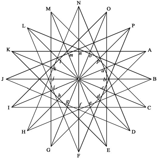
To better fix the results above and suggest alternative outlooks, the geometric methods described in [13] can be directly applied to a single diagram such as the compass rose, given in Figure 1. For each of these no-go proofs, the starting assumption is that there is some joint probability across a collection of projector triples, those used in the construction. Indeed, these Sudoku-like arguments quickly generate conflicts between classical probability and quantum outcomes.

Figure 1. Compass rose used for constructing new demonstrations of the conflict, under quantum noncontextuality, between classical probability and quantum outcomes; See Section 6 for details.

Figure 1. Compass rose used for constructing new demonstrations of the conflict, under quantum noncontextuality, between classical probability and quantum outcomes; See Section 6 for details.

More precisely, all the arguments depend on QNC(Prob) and classical probability as above, to generate an assignment of zero or one to each of the projectors in the diagram. Since QNC(Prob) and classical probability was shown above to imply commutativity of all observables, getting a contradiction within the diagram is equivalent to showing observables usually do not commute. Or, starting from QNC(Value), and an assumed classical joint probability for a nonorthogonal pair of projectors, the geometric reasoning applies directly. In which case, a conflict in the diagram only confirms, once more, that quantum observables usually do not commute.

A worked example is provided below, and a challenge to the reader is then offered.

Begin by recalling the original geometric construction in ([14]; and Section 3, above). In Hilbert space H with inner product $\langle x,y\rangle$. consider real subspace M ⊆ H for dim M = 3. Assume $x\in M,\hspace{0.17em}\langle x,x\rangle =1,$ and define affine space S(x) ⊆ M by,

$$S(s)=\{h\in M|\langle x,h\rangle =1\}$$

(11)

Observe that S(x) is a two-dimensional hyperplane in M, having as “origin” the distinguished point x.

In S(x) draw the compass rose as given in Figure 1. By construction all points connected by a line segment not passing through x are orthogonal vectors in M, as are all points on the inner circle connected by a line through x.

Let x be associated with projector observable P_x. If tr[DP_x] ≠ 0 then there exists a point ω in a corresponding sample space such that v(x) = 1, using notation as in Section 3. Continuing, results there show that the collection of vectors in the compass rose, and all required vector triples implied by arguments in Section 3, above, can be embedded in a sample space framework with at least one consistent classical joint distribution over the set. The results of [13] imply the following Assignment Rules for points in the diagram:

(1)

For any outer line segment, those ending in two upper case letters (such as A, n, K): A + K = n;

(2)

For any inner line segment, those ending in two lower case letters (such as n, x, f): n + f = x;

(3)

If a lower case (inner) letter is assigned 0, then the corresponding upper case (outer) letter must also be assigned 0. If the lower case letter is 1, then the upper case letter may be 0 or 1.

Simplifying notation, and without loss of generality, starting assignments for the diagram can be these: x = 1, A = 1, n = 1, K = 0, C = 0, f = 0, I = 0.

Examples for Applying the Rules:

(a)

For Rule (1): for A = 1, K = 0 then n = 1; if A = 1, n = 1 then K = 0. Also, for f = 0, it follows that I = C = 0;

(b)

For Rule (2): n + f =1, with n = 1 implies f = 0;

(c)

For Rule (3): if A = 1 then a =1.

An Example of a Compass Rose Collision: Without loss start with A = 1, K = 0, n = 1, f = 0, C = 0, I = 0. Drop a perpendicular from E to line segment xF; call this point F*. If E = 1 then F* = 1, contradiction (since f = 0). So E = 0. This implies h = 0 (since K = 0) so that p = 1, and M = 1 (since C = 0), so j = 1 and this implies b = 0. Drop a perpendicular from A to line segment xB; call this point B*. Since b = 0 it follows that B* = 0, which implies A = 0, contradiction.

A Challenge Problem: Construct a compass rose collision without using Rule (3).

7. Discussion

There are several ways to study connections between classical probability and quantum outcomes, and these have multiple points of tangency with the project considered here. A core theme through this material is the identification and removal of unnecessary assumptions, those that are seemingly required to obtain many hidden variable no-go proofs. It is hoped that such pruning and simplification leads to a better understanding of what is classical and what is quantum, and perhaps what should be considered classical or quantum.

One such approach has been described in [10,11], that looked at the Kochen-Specker version of a hidden variable model. The basic KS assumptions are of a supervening classical probability space for quantum observables, such that values at every point in the sample space respect commuting sums or products. This was shown in [10] to imply commutativity for all observables, and was subsequently sharpened in [11], that studied the construction of specific projectors and selected quantum states that lead to collision with the KS rules. An alternative derivation of the main result was provided in [19], but it is noted that a somewhat different conclusion regarding quantum local realism was obtained there, different from that suggested in [10,11].

Note importantly that the KS formalism has not been assumed in the current project. Thus it is not assumed that joint probability distribution is available with all quantum observables represented as random variables on a single classical probability space, and also such that any commuting pair also obeys the sum or product rule. On the other hand, the same result as in [10,11] was obtained here, using only the application of classical probability as given in Lemma 1 above, applied to specific, countable sets of observables. Moreover, the assumption of the sum and product rule for commuting observables is also not necessary in order to end with a no-go proof along the lines of the KS argument, and indeed to end with commutativity for quantum observables. Summarizing this outcome is that the assumptions of the KS formalism are unnecessary for obtaining commutativity: only the property of QNC(Prob), that is this basic result from classical probability, is all that is required.

Another approach to the contact problem effectively starts with a consequence of a classical probability space, namely the classical property of value definiteness, where at each point in the sample space, and simultaneously, every random variable takes on, or is assigned, an allowed value. Assume further that all outcomes respect orthogonality. This was studied in [14], leading to a no-go result, and methods used there were deployed above in Theorem 1. Indeed, a central task of the current project was the construction, under QNC(Prob), of a consistent joint probability distribution across a selected set of projectors that, further, satisfied orthogonality within the selected sets. Still, to be clear, it was also not assumed in the results derived here that all quantum observables should correspond to classical random variables.

Note that assuming just value definiteness as just given, is the hypothesis of QNC(Value), also called the noncontextuality of results. And this was shown here to imply commutativity for any pair of nonorthogonal projectors.

In all the results obtained here and the related results mentioned so far, no requirement is made for compound systems or any study necessary for outcome over separated systems, with or without entanglement. The algebraic consequences of the invariance of marginal probability, and the classical probability result in Lemma 1, are themselves sufficient to drive the argument to commutativity.

More generally, the existence of a contact problem between measure theory and the intuitive understanding of geometry was displayed in the decompositions paradoxes of Hausdorff (1914) and Banach-Tarski (1924); See [17,18]. Apart from the technical link to this subject given in Theorem 3 above, a formal parallel in the present project is this: Under the assumption of the invariance for marginal probabilities—routine application of classical probability is seen in conflict with the geometric foundation for quantum mechanics, as it is represented by standard spectral measure theory for quantum observables.

On the other hand, a classical or noncontextual disposition for quantum outcomes as shown here might survive by restricting the set of observables under study, where this need not arise by limiting the size of the set or limiting it to specific sets. That is, one alternative is requiring the argument above to proceed over a specific, uncountable collection of observables. In this case the result of Lemma 5—the existence of a consistent joint distribution—might not apply, and then a conflict driven by any species of compass rose might not evolve.

As support for another direction by which a version of quantum noncontextuality could manage to survive beyond the evidently hostile environment of geometry and countability, it is known that quantum noncontextuality is provably consistent over certain countable sets of projectors. These are constructed using rationals-only projectors. Details are given in [9,10], where it is shown how to evade the constructions above by invoking a specific set of infinitely many observables built from projectors having only rational numbers for components over some basis. As observed above in the proof of Theorem 3, in order to avoid a problem with a rotation having fixed points it was necessary to use angle θ for which cos θ was transcendental. A projector triple defined by such a rotation relative to a given triple would have components that are not rational, let alone not algebraic.

The loophole being exploited is that, while evidently no physical measurement can be performed with infinite precision, it is still possible that some hypothetical countable class of physical measurement could exist over which quantum noncontextuality would still be valid and would approximate arbitrarily closely any classical measurement scheme. As discussed in [8,9], this heralds a limiting argument for some class of idealized physical measurement that may or may not be feasible or meaningful.

In work closely related to this project, by tracking the order in which measurements are made it is always possible to cast a version of the contact problem as study of the four marginal distributions over a pair of quantum observables, two for each observable separately and for the two conditional measurements. Properties of quantum conditional distributions and marginal probabilities for these conditionals are discussed, for example in [13]. The agreement of these four marginals with observation can imply, or disallow, a classical probability distribution for the pair of outcomes. This has been examined in [20]. As noted following Lemma 1, no versions, conditions, or properties of quantum conditional probability and any links to classical conditional property are invoked or required for the results obtained here.

Finally, there are still other avenues for study of the contact between classical and quantum outcomes. Among these are alternative approaches to quantum field theory, and here a notable example is the work of Wetterich [21,22]; see especially the references therein. This is not easily summarized here and is properly the subject for another conversation.

References

- Spekkens, R.W. Contextuality for preparations, transformations and unsharp measurements. 2005; arXiv:0406166v3. [Google Scholar]
- Spekkens, R.W. Negativity and contextuality are equivalent notions of nonclassicality. 2008; arXiv:0710.5549v2. [Google Scholar]
- Cabello, A.; Badziąg, P.; Cunha, M.T.; Bourennane, M. Simple hardy-like proof of quantum contextuality. 2013; arXiv:1310.8330v1. [Google Scholar]
- Kleinmann, M.; Budroni, C.; Larsson, J.; Gühne, O.; Cabello, A. Optimal inequalities for state-independent contextuality. Phys. Rev. Lett. 2012, 109, 250402. [Google Scholar] [CrossRef] [PubMed]
- Kurzyński, P.; Cabello, A.; Kaszlikowski, D. Fundamental monogamy relation between contextuality and nonlocality. 2013; arXiv:1307.6710v1. [Google Scholar]
- Liang, Y.-C.; Spekkens, R.W.; Wiseman, H.M. Specker’s parable of the over-protective seer: A road to contextuality, nonlocality and complementarity. Phys. Rep. 2011, 506, 1–39. [Google Scholar] [CrossRef]
- Lisoněk, P.; Badziąg, P.; Portillo, J.R.; Cabello, A. The simplest Kochen-Specker set. 2013; arXiv:1308.6012v1. [Google Scholar]
- Kent, A. Noncontextual hidden variables and physical measurements. Phys. Rev. Lett. 1999, 83, 3755–3757. [Google Scholar] [CrossRef]
- Barrett, J.; Kent, A. Noncontextuality, finite precision measurement and the Kochen-Specker theorem. Stud. Hist. Philos. Modern Phys. 2004, 35, 151–176. [Google Scholar] [CrossRef]
- Malley, J.D. All quantum observables in a hidden-variable model must commute simultaneously. Phys. Rev. A 2004, 69, 022118. [Google Scholar] [CrossRef]
- Malley, J.D.; Fine, A. Noncommuting observables and local realism. Phys. Lett. A 2005, 347, 51–55. [Google Scholar] [CrossRef]
- Fine, A. Joint distributions, quantum correlations, and commuting observables. J. Math. Phys. 1982, 23, 1306–1310. [Google Scholar] [CrossRef]
- Beltrametti, E.G.; Cassinelli, G. The Logic of Quantum Mechanics; Addison-Wesley: London, UK, 1981. [Google Scholar]
- Malley, J.D. The collapse of Bell determinism. Phys. Letts. A 2006, 359, 122–125. [Google Scholar] [CrossRef]
- Brunet, O. A priori knowledge and the Kochen-Specker theorem. Phys. Lett. A 2007, 365, 39–43. [Google Scholar] [CrossRef]
- Gudder, S.P. Stochastic Methods in Quantum Mechanics; North Holland: Amsterdam, the Netherlands, 1979. [Google Scholar]
- Wagon, S. The Banach-Tarski Paradox; Cambridge University Press: Cambridge, UK, 1985. [Google Scholar]
- Churkin, V.A. A continuous version of the Hausdorff-Banach-Tarski paradox. Algebra Log. 2010, 49, 91–98. [Google Scholar] [CrossRef]
- Stairs, A.; Bub, J. On local realism and commutativity. Stud. Hist. Philos. Modern Phys. 2007, 38, 863–878. [Google Scholar] [CrossRef]
- Malley, J.D.; Fletcher, A. Joint distributions and quantum nonlocal models. Axioms 2014, 3, 166–176. [Google Scholar] [CrossRef]
- Wetterich, C. Quantum field theory from classical statistics. 2011; arXiv:1111.4115v1. [Google Scholar]
- Wetterich, C. Zwitters: Particles between quantum and classical. Phys. Lett. A 2012, 376, 706–712. [Google Scholar] [CrossRef]
© 2014 by the authors; licensee MDPI, Basel, Switzerland. This article is an open access article distributed under the terms and conditions of the Creative Commons Attribution license (http://creativecommons.org/licenses/by/3.0/).
Share and Cite
MDPI and ACS Style
Malley, J.D. Classical Probability and Quantum Outcomes. Axioms 2014, 3, 244-259. https://doi.org/10.3390/axioms3020244
AMA Style
Malley JD. Classical Probability and Quantum Outcomes. Axioms. 2014; 3(2):244-259. https://doi.org/10.3390/axioms3020244
Chicago/Turabian StyleMalley, James D. 2014. "Classical Probability and Quantum Outcomes" Axioms 3, no. 2: 244-259. https://doi.org/10.3390/axioms3020244